STATISTICAL ANALYSIS OF RELATIONAL DATA: MINING AND MODELING COMPLEX NETWORKS
James David Wilson
A dissertation submitted to the faculty of the University of North Carolina at Chapel Hill in partial fulfillment of the requirements for the degree of Doctor of Philosophy in the Department
of Statistics and Operations Research (Statistics).
Chapel Hill 2015
ABSTRACT
JAMES DAVID WILSON: Statistical analysis of relational data: mining and modeling complex networks
(Under the direction of Andrew B. Nobel and Shankar Bhamidi)
Networks have created many new and exciting areas of scientific inquiry, particularly in the field of statistics. The relational and often complex nature of network data requires the development of new statistical techniques that address analysis, modeling, and simulation. In this dissertation, we make contributions to the development and application of statistical methodology on network data. This work is divided into two related areas.
The first part of the dissertation is devoted to the problem of community detection: the unsu-pervised clustering of vertices in a network. Community detection is a common and important first step in the analysis of networks because networks tend to cluster into densely connected groups of vertices that often closely associate with important physical patterns of a modeled system. We develop and evaluate two novel significance-based detection techniques - the Extraction of Statisti-cally Significant Communities (ESSC) algorithm, and Multilayer Extraction. The ESSC algorithm is a hypothesis testing approach for undirected networks, while Multilayer Extraction is a score-based approach that identifies significant vertex-layer communities in multilayer networks. The performance and potential use of both methods are investigated through simulations and real data applications, and large graph consistency is established for the Multilayer Extraction algorithm.
ACKNOWLEDGEMENTS
I am incredibly fortunate to have had so many wonderful and influential people in my life. It would be impossible to acknowledge all of those who have had a significant impact on me during my graduate studies, as expressing my gratitude to these folks would take perhaps as many pages as this dissertation itself. Having said this, I will do my best to summarize.
I would not be where I am today without the love and support of my parents James and Carolyn Wilson. You have instilled in me a self-motivation and hard work ethic that has carried me through most of my personal and academic endeavors, and most importantly, you taught me how to enjoy life for all of the small things. Your regular visits to Chapel Hill were always a welcome retreat from the sometimes painstaking process of research. I will be forever grateful to you for your selfless acts and hard work on helping me discover where I fit into this world.
To my brother Jacob: I express sincere gratitude for your support and for always challenging me to do my absolute best. Beyond being my older brother, Jacob is a true friend. Without even always being fully aware of it, you taught me valuable lessons in life. From teaching me “preschool” when I could barely speak, to selflessly attending my thesis defense without having formal training in statistics, you have always been there when I needed you most.
I am grateful to my fianc´ee Rosie, whose love, support, and great patience over the last 3 years has been indespensible to my surviving graduate school. Your adventurous personality has led me to enjoy things in life that I would not have even known about without you. I cannot put into words how much I look forward to starting the next pages of our lives in San Francisco. I am the luckiest man in the world to have such an intelligent, sincere, and caring partner with whom I can share my life.
take life a little less seriously every now and then. I will miss the drinks, coffee breaks, games, and many discussions that we’ve all had, and I hope that these continue as we all go to our next stages in life.
TABLE OF CONTENTS
1 INTRODUCTION . . . 1
1.1 Network Model Types . . . 2
1.2 Significance-based Community Extraction . . . 3
1.3 GERGMs: Inference for Weighted Networks . . . 7
1.4 Outline of this Dissertation . . . 9
2 EXISTING COMMUNITY DETECTION METHODS . . . 10
2.1 Undirected Networks . . . 10
2.2 Multilayer Networks . . . 13
3 TESTING BASED EXTRACTION . . . 15
3.1 Introduction . . . 15
3.1.1 Notation . . . 15
3.1.2 Organization of the Chapter . . . 16
3.2 The ESSC Algorithm . . . 16
3.2.1 Conditional Configuration Model . . . 16
3.2.2 Description of the ESSC Algorithm . . . 20
3.3 Competing Methods . . . 23
3.4 Real Network Analysis . . . 26
3.4.1 Caltech Facebook Network . . . 27
3.4.1.1 Quantitative Comparison . . . 28
3.4.1.2 Community Features . . . 29
3.4.2 Political Blog Network . . . 30
3.4.2.2 Political Affiliation: . . . 32
3.4.3 Personal Facebook Network . . . 32
3.4.4 Enron Email Network . . . 34
3.5 Simulation Study . . . 35
3.5.1 The LFR Benchmark . . . 36
3.5.2 Background Benchmarks . . . 37
3.5.3 Results . . . 39
3.6 Discussion . . . 42
3.7 Additional Simulations . . . 43
3.7.1 Disjoint Community Benchmarks . . . 43
3.7.2 Overlapping Community Benchmarks . . . 44
3.7.3 On the Effects ofα. . . 44
3.8 Computational Settings of Competing Detection Methods . . . 47
4 LOCAL SIGNIFICANCE IN DIRECTED NETWORKS . . . 51
4.1 Introduction . . . 51
4.2 Related Work . . . 53
4.3 Statistical Model and Framework . . . 53
4.3.1 The Directed Configuration Model . . . 53
4.3.2 Asymptotic Results and Assessing the Significance of Local Connections . . . 54
4.4 Numerical Evaluation . . . 58
4.4.1 Convergence Rate under the DCM . . . 58
4.4.2 Analysis of Networks with Directed Community Structure . . . 59
4.4.3 Political Blog Network . . . 61
4.5 Discussion . . . 63
5 MULTILAYER EXTRACTION . . . 65
5.1 Introduction . . . 65
5.2 Scoring a Vertex-Layer Group . . . 67
5.2.1 The Null Model . . . 68
5.2.2 Significance-Based Score . . . 69
5.3 Consistency Analysis . . . 70
5.3.1 Consistency of the Score . . . 71
5.4 The Multilayer Extraction Procedure . . . 72
5.4.1 Initialization . . . 73
5.4.2 Extraction . . . 73
5.4.3 Refinement . . . 75
5.4.3.1 Choice ofβ . . . 75
5.5 Real Network Analysis . . . 76
5.5.1 AU-CS Network . . . 79
5.5.2 European Air Transportation Network . . . 81
5.5.3 arXiv Network . . . 81
5.6 Simulation Study . . . 82
5.6.1 Multilayer Stochastic Block Model . . . 83
5.6.2 Persistence . . . 85
5.6.3 Single Embedded Communities . . . 86
5.6.4 Extraction Simulations . . . 87
5.7 Discussion . . . 88
5.8 Proof of Consistency. . . 89
6 STOCHASTIC WEIGHTED GRAPH MODELS . . . 96
6.1 Introduction . . . 96
6.2 The Generalized Exponential Random Graph Model . . . 97
6.3 Model Inference . . . 99
6.3.1 Maximum Likelihood Inference . . . 99
6.3.3 Simulation via Gibbs Sampling . . . 102
6.3.4 A General Inferential Framework via Metropolis-Hastings . . . 103
6.4 Flexible Model Specification . . . 105
6.5 Numerical Evaluation . . . 107
6.5.1 Application to the International Lending Network . . . 108
6.5.2 Application to U.S. Migration Network . . . 110
6.5.3 Simulation Study: Non-Degeneracy in the Two-Star Model . . . 113
6.6 Discussion . . . 116
7 FUTURE WORK . . . 118
7.1 Significance-based Community Extraction . . . 118
7.2 Statistical Inference for Weighted Networks . . . 119
LIST OF TABLES
3.1 Competing Methods Summary . . . 26
3.2 Real Application Summary . . . 27
3.3 Caltech Facebook Features . . . 27
3.4 Caltech Community Summary . . . 28
3.5 Political Blog Community Summary . . . 31
3.6 Personal Facebook Features . . . 34
3.7 LFR Benchmark Parameters . . . 36
3.8 Resolution of Caltech Communities I . . . 45
3.9 Resolution of Caltech Communities II . . . 45
3.10 Resolution of Political Blog Communities I . . . 46
3.11 Resolution of Political Blog Communities II . . . 46
4.1 Political Affiliation of Political Blogosphere . . . 63
5.1 Real Application Summary . . . 78
6.1 Flexible Network Statistics for the GERGM . . . 106
LIST OF FIGURES
1.1 Toy Network with Three Disjoint Communities . . . 4
1.2 Enron Email Network . . . 5
3.1 Caltech Community Sizes . . . 29
3.2 Caltech Classification Results . . . 31
3.3 Personal Facebook Network . . . 33
3.4 Extraction Benchmark Results . . . 40
3.5 Disjoint + Background Benchmark Results . . . 41
3.6 Disjoint Benchmark Results . . . 49
3.7 Overlapping Benchmark Results . . . 50
4.1 Local Connections in Directed Networks . . . 52
4.2 Convergence Rate Analysis . . . 59
4.3 The Stochastic Co-Blockmodel . . . 60
4.4 Co-Blockmodel Benchmark Results . . . 61
4.5 Co-Blockmodel Local Connection Strengths . . . 61
4.6 Political Blog Local Connection Strengths . . . 63
4.7 Political Affiliation of Political Blogosphere . . . 64
5.1 Summary of Real Application Results . . . 78
5.2 Match Between Methods in Real Applications . . . 79
5.3 Multilayer Applications . . . 80
5.4 Simulation Results . . . 84
5.5 Extraction Simulation Test Bed . . . 87
6.1 International Lending Network Goodness of Fit . . . 109
6.2 International Lending Network Traceplots . . . 110
6.4 U.S. Migration Network Goodness of Fit . . . 113
6.5 In Two Stars Degeneracy Plots . . . 114
6.6 Non-degenerate In Two Stars Simulation . . . 115
CHAPTER 1: INTRODUCTION
The study of networks, collectively referred to as network science, has made significant contri-butions to the modeling and understanding of complex systems. The mathematical foundation of network analysis is rooted in graph theory, whose origin is widely attributed to Leonhard Euler’s resolution of the “Seven Bridges of K¨onigsberg” problem in 1735. In his analysis, Euler was the first to represent an observed system as a collection of vertices (land masses) connected by edges (bridges). Since then, network analytic techniques have been successfully applied in a number of diverse settings, including biology to model protein-protein and gene-gene interactions (Levy and Pereira-Leal, 2008); in sociology to model friendship and information flow among a group of individuals (Wasserman, 1994); and in neuroscience to model the relationship between the orga-nization and function of the brain (Sporns, 2011). In industry, technology companies like Google, Facebook, and Microsoft employ network methodology for a variety of applications such as social network analysis, recommender systems, and marketing. As underscored by these diverse applica-tions, the dozens of network-driven computer science conferences held each year, and the creation of two stand-alone network journals in 2013, network science is a flourishing field that spans many scientific areas.
treatment on the statistical analysis of networks is provided by Kolaczyk (2009), and the surveys, Goldenberg et al. (2010) and Fienberg (2012), provide two recent resources on the topic.
Our primary contributions are to the development and application of statistical methodology for complex network data. This work can be divided naturally into two areas. We first consider the problem of clustering the vertices of an observed graph. This unsupervised task, known com-monly as community detection, is a well-explored topic for which a variety of methods have been developed. Notably, existing community detection methods do not address the statistical quality of identified communities. Moreover, a majority of existing community detection methods implicitly assume that every vertex of a network belongs to at least one community. These considerations are especially important in the multilayer network setting, where community structure often dif-fers from layer to layer. In the first part of this dissertation, we develop two significance-based exploratory techniques - the Extraction of Statistically Significant Communities (ESSC) algorithm, and Multilayer Extraction - that provide a means to assess and identify statistically significant communities in undirected and multilayer networks.
Our second contribution concerns simulating and modeling networks with weighted edges. In the social sciences, the exponential random graph model (ERGM) is a fundamental tool for statis-tical inference of network data. Despite their popularity, ERGMs have a major limitation in that they require that the edges of a modeled network are binary (representing the presence or absence of an edge). The generalized exponential random graph model (GERGM) of Desmarais and Cran-mer (2012) extends the ERGM to the family of networks with continuous-valued edges; however, current estimation procedures for the GERGM only allow inference on a restricted family of model specifications. To address this limitation, we propose and investigate a new Metropolis-Hastings procedure that greatly extends the family of weighted networks that can be modeled under the GERGM framework.
1.1 Network Model Types
a vertex set V where each vertex (node) u ∈ V represents a unit in the system, and an edge set E ⊆ V ×V that contains all pairs {u, v} such that there is a physical or functional relationship between the verticesuandv. To handle the unique structure of relational data, a variety of network models have been developed. Without loss of generality, we will enumerate the vertices inV with numbers [n] = {1, . . . , n}. Throughout this dissertation, we will consider four types of network models:
Undirected, Unweighted Networks: relationships are symmetric and binary so that {u, v} ∈ E implies that theu, v∈[n] share a mutual relationship.
Directed, Unweighted Networks: relationships are asymmetric and binary so that (u, v) ∈ E implies thatu∈[n] is related tov∈[n] and that an edge pointsfromu to v.
Multilayer Networks: represented by a collection G(m, n) = (G1, . . . , Gm) of m undirected,
simple graphs G` = ([n], E`). The graphG` is referred to as a layer. The indexing of layers by
`∈[m] is arbitrary, and does not reflect an underlying spatial or temporal order. We treat the vertices as registeredso that actor u∈[n] is the same entity across layers. Thus the graph G`
reflects the relationships between identified actors 1, . . . , nin circumstance `.
Weighted Networks: relationships can be symmetric or asymmetric. Each edge e(u, v) ∈ E has an associated weight w(u, v)∈(−∞,∞) that specifies the strength of connection between u, v∈[n].
In each of the above cases, a graph onnvertices can be also be represented in matrix notation via the so-called adjacency matrix. For a graph with nvertices, the adjacency matrix A = (Au,v)
is a n×nmatrix where entryAu,v denotes the edge weight between nodes u, v∈[n] (0 or 1 in the
case of unweighted graphs).
1.2 Significance-based Community Extraction
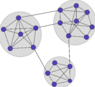
plays an important role in the exploratory analysis of network data. In the network setting, it is often the case that the vertices of a network under study cluster into so-called communities, or groups of tightly connected vertices. Informally, a community is a group of vertices that are more connected to each other than they are to the remainder of the network. More rigorous definitions quantify this notion of differential connection in different ways depending upon, for example, the type (undirected, directed, multilayer) of network under analysis. Figure 1.1 illustrates a simple undirected network with three disjoint communities.
Figure 1.1: A simple network with three distinct communities.
A majority of existing community detection methods implicitly assume that every vertex of a network belongs to at least one community. As we will see from numerous applications throughout this dissertation, networks often contain non-preferentially attachedbackgroundvertices that act as noise against which significant communities can be identified. As an example, consider the Enron email network from Leskovec et al. (2009) (Figure 1.2). The edges of this network represent the email correspondence (sent or received) between email accounts in 2001. The network contains many (on the order of 10K) email accounts outside of Enron and relatively few (on the order of 1K) email accounts from employees at Enron. The outside email accounts, many of which are spam email accounts, are not preferentially attached to any group of employees and thereby do not belong to a well-defined community. Existing detection methods typically seek a partition or cover of the vertices, which in cases like the Enron data set, can lead to false discovery and misleading conclusions.
Figure 1.2: The Enron Email Network. Nodes are colored according the partition of vertices identified by Spectral Clustering. This network contains many non-preferentially attached vertices.
We begin with an observed network onnvertices. To identify statistically relevant community structure, we proceed in three distinct steps. First, we model the observed network using an appropriate random graph model, namely, a probability measure on the family of graphs with n vertices. We choose a model that dictates non-preferential connection between the n vertices while maintaining the degree distribution of the observed graph. Properties of fixed degree random graph models have been thoroughly investigated in probability and statistics (Durrett et al., 2007; Blitzstein and Diaconis, 2011), and they also play an important role in community detection, particularly in the development of modularity-based detection methods (Newman, 2006b). Our chosen random graph model serves as a null model with which we compare our observed graph.
The next step requires the specification of a network statistic that describes the connectivity of a candidate community. For an undirected network G= ([n], E), we quantify the attraction of a node u ∈ [n] and a vertex collection B ⊆ [n] via the observed number of connections between u and B, dn(u : B). Let dbn(u : B) denote the expected number of these connections under the
corresponding random graph model. Suppose that the number of edges incident to a node u, i.e. its degree, is given by dn(u). Then under suitable conditions,
DT V
b
dn(u:B),Binomial(dn(u), pn(B))
→0, asn→ ∞ (1.1)
whereDT V(·,·) is the usual total variation distance andpn(B) is the relative volume of the collection
B. Using the binomial distribution as a reference, we quantify the strength of connection between
u and B through the approximate p-value
p(u:B) :=P r(dbn(u:B)>dn(u:B))
According to (1.1),p(u:B) can be calculated using a simple binomial tail probability. Small values of p(u :B) suggest significant connections between u and B. In practice, this local evaluation of significance can be utilized in both undirected and directed networks. We go in more detail about this in Chapters 3 and 4.
be the expected number of such edges under a fixed degree multilayer random graph model. We compare y(B, L) withY(B, L) using the following probability bound:
P r(Y(B, L)> y(B, L))6exp{−S(B, L)} (1.2)
We use the the exponentS(B, L) in (1.2) to score the overall connectivity of a vertex layer group (B, L). Large values ofS(·,·) are associated with densely connected collections.
In our final step, we develop algorithms to identify statistically significant communities. In undirected networks, we seek collections B∗ such that the p-value p(u:B∗) is small for allu∈B∗ and the p-value p(v:B∗) is large for allv /∈B∗. We develop the iterative and testing-based ESSC algorithm to identify these significant communities. On the other hand, in multilayer networks, the goal is to identify vertex layer groups (B, L) with large score S(B, L). To that end, we develop the Multilayer Extraction algorithm to identify significant vertex-layer groups. Both ESSC and Multilayer Extraction are based on a family of detection algorithms known ascommunity extraction procedures. Community extraction is the iterative search for densely connected communities, which are identified one at a time. Extraction methods can readily handle overlapping and disjoint community structure, and these methods do not require that every vertex of a graph belongs to a community. Extraction has recently been explored in standard (single-layer) networks by Zhao et al. (2011); Lancichinetti et al. (2011), and Wilson et al. (2014).
1.3 GERGMs: Inference for Weighted Networks
A fundamental tool for the statistical analysis of networks is the exponential random graph model (ERGM) - a popular, powerful, and flexible tool for statistical inference of network data (Holland and Leinhardt, 1981; Wasserman and Pattison, 1996; Snijders et al., 2006). The ERGM is a probability measure on the family of graphs with vertex set [n] that incorporates relational structure between the vertices to generate a random vector of edgesX∈Rm. This probability distribution is
specified by a joint probability density functionfX(x,Θ), which is driven by a function of summary
modeled by an exponential family with parametersθθθ∈Rp as follows:
fX(x, θθθ) =
exp (θθθ0hhh(x))
R
[0,1]mexp (θθθ0hhh(z))dz
, x∈ {0,1}m (1.3)
Model (1.3) can be used to capture various dependence relationships of X including, for ex-ample, reciprocity, preferential attachment, and transitivity. As ERGMs require that the edges of an observed network are binary, they are unable to model weighted networks. Since many sub-stantively important networks are weighted, this restriction is especially problematic. Weighted networks arise, for example, in the study of financial exchange (Iori et al., 2008), migration pat-terns (Chun, 2008), and in the analysis of brain functionality and connectivity (Simpson et al., 2011).
Recently, some progress on modeling weighted networks in the ERGM framework was made in Desmarais and Cranmer (2012), where the generalized exponential random graph model (GERGM) was proposed to study networks with continuous-valued edges. Furthermore, Krivitsky (2012) developed a weighted exponential random graph model that generalized the ERGM to networks with discrete-valued (i.e., count) edges. Though both models provide a means to analyze weighted networks, we focus on flexible specifications of the GERGM.
In general, the likelihood function of an ERGM is intractable; however, efficient estimation can be achieved through the use of Markov Chain Monte Carlo (MCMC) algorithms (Geyer and Thompson, 1992; Hunter and Handcock, 2006). As the target probability density is an exponential family, MCMC can be used to simulate samples of networks from which the likelihood function of an ERGM can be approximated. Like the ERGM, estimation of the GERGM is readily achieved via MCMC algorithms. Desmarais and Cranmer (2012) proposed a Gibbs sampling technique for GERGM estimation; however, this strategy limits the specification of network dependencies captured by the GERGM.
probable, estimation via MCMC will fail to converge to consistent parameter estimates. In the instance of binary networks, scholars have attempted to resolve the issue of degeneracy by using network statistics that closely correspond to conditionally independent specifications in Markov graphs (Frank and Strauss, 1986). Unfortunately, as pointed out in Snijders et al. (2006) and Hunter et al. (2008), these models largely restrict the number of permissible underlying subgraph configurations in the observed network.
To address the issues of the model specifications in Desmarais and Cranmer (2012), in Chapter 6 we expand the family of weighted networks that can be analyzed under the GERGM by developing a Metropolis-Hastings sampling procedure that allows the flexible specification of network statistics and models under the GERGM framework. Under our proposed Metropolis-Hastings procedure, we show that one can avoid degeneracy in cases where previously specified model specifications were not able.
1.4 Outline of this Dissertation
CHAPTER 2: EXISTING COMMUNITY DETECTION METHODS
In this chapter, we describe existing community detection methods for undirected and multi-layer networks. We highlight key methodologies that have most influenced the development and application of community detection. For recent surveys describing community detection in undi-rected networks, see Fortunato (2010) and Porter et al. (2009).
2.1 Undirected Networks
Existing community detection methods capture different types of community structure. The sim-plest community structure, and the one most commonly studied, is a hard partitioning, in which each vertex of the network is assigned to one and only one community, and the collection of commu-nities together form a partition of the network (e.g, Newman and Girvan (2004); Ng et al. (2002); Snijders and Nowicki (1997)). Another class of community structure allows overlapping commu-nities (Xie and Szymanski, 2011), in which the collection of commucommu-nities together form a cover of the network. Broadly speaking, most community detection methods produce one of these types of structure. For ease of discussion, in each of the following descriptions we will suppose that we observe an undirected graph Gwithn vertices and degree sequence{d1, . . . , dn} where the degree
du is simply the number of edges incident onu. LetA be the adjacency matrix associated withG.
One prominent class of community detection methods are based on the spectral properties of a network. Let D=diag(d1, . . . , dn) denote the degree matrix of G. There is an extensive literature
fact that it can be used to solve a relaxed form of the graph partitioning problem originating from the min-cut and max-flow problem (Goldberg and Tarjan, 1988), where one seeks a partition of k communities that contain the smallest number of inter-community edges. Often, the partition that optimizes the min-cut max-flow criterion contains trivial singleton communities. In light of this shortcoming, the ratio-cut and normalized-cut criterions were introduced to deal with this issue (Wei and Cheng, 1989; Shi and Malik, 2000). A number of heuristics have been proposed to determine the number of communities k(e.g., the spectral gapmethod (Von Luxburg, 2007)), but this problem is still a subject of open research. One notable variant of spectral clustering is the method described in Newman (2006a), which instead evaluates the graph Laplacian of the so-called modularity matrix derived from the modularity of a partition.
A second important class of community detection methods seek a partition of the vertices [n] that maximize the quality function known as modularity. Let M =P
u∈[n]du denote the total of number of edges inG. Then the modularity of a partition is given by
Q= 1 2M
X
u,v∈[n]
Au,v−
dudv
2M
δu,v
whereδu,v indicates whether or not u andv are in the same community. In words, the modularity
Q measures the degree to which the organization of a partition differs from what is expected under a null random graph model. The quantity dudv
2M is the expected edge weight between two
vertices u, v ∈ [n] if the vertices were randomly connected according to the Chung-Lu random graph (Aiello et al., 2000). Optimizing Q is an NP-hard problem; however, an extensive number of computational algorithms have been developed to approximate the optimal partition (Blondel et al., 2008; Clauset et al., 2004; Newman, 2006b; Mucha et al., 2010). The most popular way to search for a partition with optimal modularity involves an adaptation of the agglomerative algorithm known as the Kernighan-Lin algorithm (Kernighan and Lin, 1970), though a wide array of other algorithms have been developed for this purpose.
An alternative class of community detection methods involves the estimation of community structure in a network via likelihood maximization. For this, one specifies a random graph model, typically some variant of the stochastic block model (SBM), which is a probability measurePon the
vertices of the same community are preferentially attached (Wang and Wong, 1987; Snijders and Nowicki, 1997). One then estimates the community labels of each vertex by maximizing the likeli-hood underP. Traditionally, the stochastic block model characterizes disjoint community structure;
however, recent development has lead to more nuanced models include latent variable models (Hoff et al., 2002; Handcock et al., 2007) and mixed membership models for overlapping community structure (Airoldi et al., 2008; Ball et al., 2011). Recently, there has been significant progress in the development of fast and efficient algorithms for fitting stochastic block models. Decelle et al. (2011b) describes an algorithm that estimates block structure of a degree-corrected block model in time linear in the number of vertices. Their algorithm is based on a powerful heuristic of belief propagation from statistical physics. A sublinear algorithm based on the pseudo-likelihood of the sparse block model is described in Amini, Chen, Bickel, Levina et al. (2013), wherein block labels are shown to be consistent in the size of the network. Finally, recent nonparametric representa-tions of the blockmodel through dense graph limits, or graphons, (Airoldi et al., 2013) and network histograms (Olhede and Wolfe, 2013) provide promising new directions for the understanding and estimation of block models.
Community extraction techniques provide another subclass of detection methods. Community extraction is the iterative search for densely connected communities, which are identified one at a time. Extraction has been recently explored in undirected networks by Zhao et al. (2011), Lancichinetti et al. (2011), and Wilson et al. (2014). Rather than search for an optimal partition or cover, these extraction methods seek the strongest connected community sequentially. Extraction methods do not force all vertices to be placed in a community and thereby are flexible to loosely connected background vertices. Extraction techniques are particularly well-suited for networks in which there belong many non-preferentially attached vertices. Our developed methodology, ESSC and Multilayer Extraction, both belong to this class of community detection techniques.
the-oretical questions remain open for these types of methods including convergence of bootstrapped samples of networks.
2.2 Multilayer Networks
While there is a large and growing literature of community detection methods devoted to a single network, the development of community detection methodology in multilayer networks is still in its infancy. Here, we describe the general approaches used to identify community structure in multilayer networks. Throughout, suppose that we observe a multilayer network G(m, n) with n nodes andmlayers. Multilayer network models have been applied to a variety of problems, including modeling and analysis of air transportation routes (Cardillo et al., 2013), studying individuals with multiple sociometric relations (Fienberg et al., 1980, 1985), and analyzing relationships between social interactions and economic exchange (Ferriani et al., 2013). Kivel¨a et al. (2014) and Boccaletti et al. (2014) provide two recent reviews of multilayer networks, as well as a survey of open research questions. Below, we give an overview of the literature on community detection methods for multilayer networks.
Holland et al. (1983) first proposed a multigraph version of the stochastic block model, which is a generative model for multilayer networks that enforces preferential attachment among vertices of the same community. Recently, Paul and Chen (2015) introduced a multilayer stochastic block model. This model is a multilayer generalization of the well-known stochastic block model (SBM) (Wang and Wong, 1987; Snijders and Nowicki, 1997), which is a popular likelihood-based detection method for single-layer networks. Multigraph stochastic block models have recently been used for the theoretical analysis of multilayer community detection algorithms (Han et al., 2014). Like the single-layer SBM, multilayer block models can be used to identify community structure in multilayer networks via likelihood maximization.
methods identify a family of communities (V1,[m]), . . . ,(Vk,[m]) where V1, . . . , Vk form a partition
or cover of the vertex set [n], and each community contains all layers. When the layers ofG(m, n) all have the same, or very similar, community structure, aggregate approaches borrow strength across layers, and tend to perform well. However, aggregate methods do not discriminate between layers and therefore are likely to provide misleading results when the layers ofG(m, n) have heterogenous community structure.
Another approach to multilayer community detection is to apply a single network detection method to each layer of the observed network. Layer-by-layer methods have recently been used in Barigozzi et al. (2011), and Berlingerio et al. (2013). In these applications, each layer was treated independently with no regard to other layers. In principle, one could combine the resulting communities using some frequent pattern matching or consensus clustering approach; however, to the best of our knowledge this has not been done in practice.
CHAPTER 3: TESTING BASED EXTRACTION1
3.1 Introduction
We begin by investigating the community structure of undirected networks. In this regime, edges are symmetric in the sense that the relationship between any two linked vertices is mutual. In this chap-ter, we propose and study a testing based community detection algorithm for undirected networks, called Extraction of Statistically Significant Communities (ESSC), that is capable of identifying overlapping community structure, and can distinguish non-preferentially attached background ver-tices from significant communities. The core of the algorithm is an iterative search procedure that identifies statistically stable communities. In particular, the search procedure uses tail probabili-ties derived from a stochastic configuration model based on the observed network in order to assess the strength of the connection between a single vertex and a candidate community. Updating of the candidate community is carried out using ideas from multiple testing and false discovery rate control.
The only free parameter in the ESSC algorithm is a false discovery rate threshold that is used in the update step of the iterative search procedure. The number of detected communities, their overlap (if any), and the size of the background are handled automatically, without user input. In practice, the output of ESSC is not overly sensitive to the threshold parameter; see Section 3.7.3 for more details.
3.1.1 Notation
For ease of discussion throughout the remainder of this chapter, we first introduce some notation. Let G = (V, E) be an undirected graph with vertex set V = [n] = {1, . . . , n} and edge set E containing all (unordered) pairs{i, j}such that there is an edge between verticesiand jinG. Let
1Much of this chapter is reproduced from the published manuscript ”A testing based extraction algorithm for
d(u) denote the degree of a vertex u, and let d = {d(1), . . . , d(n)} denote the degree sequence of G. Let B ⊂ [n] denote a subset of vertices in G. Indices on B are simply used for specification throughout. We will useGo to denote an observed graph andGb for a random graph on the vertex
set [n].
3.1.2 Organization of the Chapter
Section 3.2 is devoted to a detailed description of our proposed algorithm for extraction of sta-tistically significant communities (ESSC), including motivation and a description of the reference distribution generated from the configuration model.
In Section 3.4 we apply the ESSC algorithm to four real world networks. These results provide compelling evidence that ESSC performs well in practice, is competitive with (and in some cases arguably superior to) several leading community detection methods, and is effective in capturing background vertices. In Section 3.5 we propose a test bed of benchmark networks for assessing the performance of detection methods specifically on networks with background vertices. To the best of our knowledge, this is the first set of benchmarks proposed for networks of this type. We show that ESSC outperforms existing methods on these background benchmarks. We also show that ESSC performs competetively on standard (non-background) benchmark networks with both non-overlapping and overlapping community structures. We end with a discussion of our work and avenues for future research.
3.2 The ESSC Algorithm
3.2.1 Conditional Configuration Model
Let Go be an observed, undirected network having n vertices. Though many networks of interest
will be simple,Go may contain self-loops or multiple edges. Assume without loss of generality that
Go has vertex set V = [n] = {1,2, . . . , n}. The edge multiset Eo of Go contains all (unordered)
pairs{i, j}such thati, j∈[n] and there is an link between verticesiandj inGo, with repetitions
for multiple edges. Letdo(u) denote the degree of a vertex u, that is, the number of edges incident
The starting point for our analysis is a stochastic network model that is derived from the degree sequence do of Go, specifically, the configuration model associated with do, which we denote by
CM(do) (Bender and Canfield (1978), Bollob´as and Universitet (1979), Molloy and Reed (1995)).
The configuration model CM(do) is a probability measure on the family of multigraphs with vertex
set [n] and degree sequencedothat reflects, within the constraints of the degree sequence, a random
assignment of edges between vertices.
The configuration model CM(do) has a simple generative form. Initially, each vertex u∈[n] is
assigneddo(u) “stubs”, which act as half-edges. At the next stage, two stubs are chosen uniformly
at random and connected to form an edge; this procedure is repeated independently until all stubs have been connected. Let Gb = ([n],E) denote the random network generated by this procedure.b
Note that Gb may contain self loops and multiple edges between vertices, even if the given network
Gis simple.
The configuration model CM(do) is capable of capturing and preserving strongly heterogeneous
degree distributions often encountered in real network data sets. Importantly, all edge probabilities in the configuration null model are determined solely by the degree sequence do of an observed
graph. As a result, fitting a configuration model does not rely on simulation; rather, estimation only requires the degree sequence of a single observed graph.
Under the configuration model CM(do) there are no preferential connections between vertices,
beyond what is dictated by their degrees. As such, CM(do) provides a reference measure against
which we may assess the statistical significance of the connections between two sets of vertices in the observed networkGo: the more the observed number of cross-edges deviates from the expected
number under the model, the greater the significance of the connection between the vertex sets. Let the observed network Go and the random network Gb be as above. Given a vertex u∈[n] and
vertex setB ⊆[n] let
do(u:B) = X
v∈B X
e∈Eo
I(e={u, v})
denote the number of edges between u and some vertex in B in Go. Define d(ub : B) as the
corresponding number of edges inG. Note thatb d(ub :B) is a random variable taking values in the
set{0,1, . . . , do(u)}, and that do(u:B) =d(ub :B) =do(u) whenB = [n] is the full vertex set. We
model which will form the basis of the algorithm. Recall that the total variation distance between two probability mass functions p:={p(i)}i>0 and q:={q(i)}i>0 on the space of natural numbers
Nis defined by
DT V(p,q) :=
1 2
∞
X
i=0
|p(i)−q(i)|
Theorem 3.1. Let {do,n}n>1 be the degree sequences of an observed sequence of graphs {Gno}n>1 where Gno is a graph with vertex set [n] and edge set Eo,n. Let {Gbn}n>1 be the corresponding random graphs on [n]constructed via the configuration model. Let Fn be the empirical distribution
of do,n. Assume that there exists a cumulative distribution function F on [0,∞) with 0 < µ := R
R+x dF(x)<∞ such that
Fn−→w F (3.1)
and
Z
R+
x dFn(x) → µ (3.2)
Fix k > 1. For each n > 1, let u = un ∈ [n] be a vertex with degree do,n(u) = k and let
B = B(n) ⊆ [n] be a set of vertices. Then the random variable dbn(u : B) is approximately Binomial(k, pn(B)) in the sense that
DT V(dbn(u:B),Bin(k, pn(B)))→0,
as n→ ∞. Here
pn(B) = X
v∈B
do,n(v) X
w∈[n]
do,n(w)
= 1
2|Eo,n|
X
v∈B
do,n(v), (3.3)
where |Eo,n|is the total number of edges in the graph.
Proof. Equation (3.2) implies that for the number of edges Eo,n one has Z
R
xdFn(x) =
∞
X
k=0
kNk(n) n = 2
|Eo,n|
n ∼µ
Now to understand the distribution of dbn(u :B), namely the number of connections of vertex
u to the subsetB in CM(do,n), we use the fact that for constructing the configuration model, one
can start at any vertex and start sequentially attaching the half-edges of that vertex at random to available half edges. We start with the fixed vertex u and decide the half edges paired to the do,n(u) := k half edges of vertex u. Write A1 for the event that the first half-edge of vertex v
connects to the setB and write r1(B) for the probability of this event. Then,
r1(B) =
P
v∈Bdo,n(v)
[P
v∈[n]do,n(v)]−1
=
P
v∈Bdo,n(v)
2|Eo,n| −1 (3.4)
Now if each half-stub is sampled with replacement from the stubs corresponding to set B then
b
dn(u : B) would exactly correspond to a Binomial distribution. The main issue to understand is
the effect of sampling without replacement from the half-stubs ofB, namely once a half-stub of B is used by u, it cannot be reused. In general for 16i6k, letAi denote the event that half-edge
i connects to the set B and write ri(B) for the conditional probability of Ai conditional on the
outcomes of the firsti−1 choices. Fori= 2, we claim that uniformly on all outcomes for the first edge, this conditional probability can be bounded as
[P
v∈Bdo,n(v)]−1
2|Eo,n| −2 6
r2(B)6
P
v∈Bdo,n(v)
2|Eo,n| −2
(3.5)
The lower bound arises if the first half edge of v connected to a half edge of B while the upper bound arises if the first half edge does not connect to a half edge emanating from B. Arguing analogously for 16i6k we find that the conditional probabilityri(B) that thei-th half-edge of
vertex v connects toB is bounded (uniformly on all choices of the firsti−1 edges) as
[P
v∈Bdo,n(v)]−(i−1)
2|Eo,n| −i 6ri(B)6
P
v∈Bdo,n(v)
2|Eo,n| −i (3.6)
Recall that pn(B) =Pv∈Bdo,n(v)/2|Eo,n|. Since|Eo,n| ∼nµ/2 Using (3.6) we have
sup 16i6k
|ri(B)−pn(B)|63
k 2|Eo,n|
+O
k 2|Eo,n|
2!
→0 (3.7)
Now note that the random variable of interestdbn(u:B) can be expressed as
b
dn(u:B) = k X
i=1
1{Ai}
Equation (3.7) implies that
DT V(dbn(u:B),Bin(k, pn(B)))→0, asn→ ∞.
as desired.
In light of the fact that the configuration model CM(do) does not contain preferential
connec-tions between vertices, the probabilities
p(u:B) = P(d(ub :B)>do(u:B)) (3.8)
can be used to assess the strength of connection between a vertexu and a set of vertices B ⊆[n]. In particular, small values of p(u :B) indicate that there are more edges between u and B than expected under the configuration model.
If we regard do(u : B) as the observed value of a test statistic that is distributed as d(ub :B)
under the null model CM(do), then p(u :B) has the form of a p-value for testing the hypothesis
thatu is not strongly associated withB.
This testing interpretation of p(u : B) plays a role in the iterative search procedure that underlies the ESSC method (see below). However, we note that the testing point of view is informal, as the null model CM(do) itself depends on the observed networkGothrough its degree distribution.
In general, the exact value of the probability p(u : B) in (3.8) may be difficult to obtain. In practice, the ESSC procedure approximates p(u : B) by P(XB > do(u : B)), where XB has a
Binomial(d(u), p(B)) distribution appealing to the result of Theorem 3.1.
3.2.2 Description of the ESSC Algorithm
vertices that acts as a seed, the procedure successively refines and updatesB0 using (the binomial approximation of) the probabilities (3.8) until it reaches a fixed point, that is, a vertex set that is unchanged under updating. The final vertex set identified by the search procedure is a detected community.
The Community-Search procedure is applied repeatedly across all vertex neighborhoods in an observed graph. The resulting collection C of detected communities (omitting repetitions) constitutes the output of the algorithm. The seed setB0 for the initial run of the search procedure is a vertex and all of the vertices adjacent to it.
To simplify what follows, letC1, . . . , CK be the distinct detected communities ofGo inC. The
background ofGois defined to be the set of vertices that do not belong to any detected communities:
C∗ = Background(Go :C) = [n]\ K [
k=1
Ck. (3.9)
In principle, the number K of detected communities can range from zero to n. Importantly, K is not fixed in advanced, but is adaptively determined by the ESSC algorithm. The identification of detected communities by theCommunity-Search procedure allows communities to overlap. As with the number of discovered communities, K, the presence and extent of overlap is automatic; no prior specification of overlap specific parameters are required.
The updates of theCommunity-Searchprocedure bear further discussion. Consider an ideal setting in which, for each vertex u and vertex set B we can determine, in an unambiguous way, whether or notu is strongly connected toB inGo. Informally, a set of verticesB is a community
if the verticesu∈B have a strong connection with vertices inB, while the verticesu∈Bcdo not. Equivalently, B is a community if and only if it is a fixed point of the update rule
S(A) = {u∈[n] such thatu is strongly connected withA}
(and success) of this simple procedure is assured, as the power set of [n] is finite. By the exhaustive or selective considering of appropriate seed sets we can effectively explore the space of fixed points of S(), and thereby identify communities inGo.
In practice, we make use of the probabilities{p(u:B) :u∈[n]}to measure the strength of the connection between u∈[n] andB relative to the reference distribution CM(d). In particular, we regardp(u:B) informally as a p-value for testing the null hypothesis HBu thatuis not preferentially connected toB. Then the task of identifying the verticesu preferentially connected toB amounts to rejecting a subset of the hypotheses {HB
u : u ∈ [n]}. This is accomplished in steps 4 and 5
of the Community-Search procedure, where we make use of an adaptive method of Benjamini and Hochberg (Benjamini and Hochberg, 1995) to reject a subset of the hypotheses. The rejection method ensures that the expected number of falsely rejected hypotheses divided by the total number of rejected hypotheses (the so-called false discovery rate) is at most α (Benjamini and Hochberg, 1995). A default false discovery rate threshold α of 5% is common in many applications, and we adopt this value here. Pseudo-code for the Community-Search procedure and ESSC algorithm is shown below.
Community-Search Procedure
Given: GraphGo= ([n], Eo); significance levelα∈(0,1).
Input: Seed setB0⊆[n].
Initialize: t:=−1,B−1=∅.
Loop (Update): UntilBt+1=Bt
1. t := t+1
2. Computep(u:Bt) for eachu∈[n].
3. Order thenvertices ofGoso thatp(u1:Bt)6· · ·6p(un:Bt).
4. Letk>0 be the largest integer such thatp(uk :B)6(k/n)α.
5. UpdateBt+1:={u1, . . . , uk}.
ESSC Algorithm
Input: GraphGo= ([n], Eo); significance levelα∈(0,1).
Initialize: V = [n],C:=∅.
Loop through all verticesu∈V:
Define seed setB0:={u} ∪ {v∈[n] :{u, v} ∈Eo}
Obtain communityC:=Community-Search(B0).
IfC6=∅andC6⊂ Cthen
UpdateC:=C ∪ {C}.
Repeat Loop
Return: FamilyC of unique detected communities.
3.3 Competing Methods
Here we describe the set of community detection methods that we use for validation and comparison with ESSC. We implement a variety of established detection methods all of which have publicly available code. We note that we do not compare ESSC with the recently developed fast block model algorithms from Decelle et al. (2011b), Airoldi et al. (2013) and Krzakala et al. (2013); such comparisons would be interesting for future work. The parameter settings for each algorithm are described in Section 3.8.
GenLouvain: The GenLouvain method of Jutla et al. (2011–2012) is a modularity-based method that employs an agglomerative optimization algorithm to search for the partition that maxi-mizes modularity. The algorithm is composed of two stages that are repeated iteratively until a local optimum is reached. In the first, each vertex is assigned to its own distinct commu-nity. Then for each vertex u (of community Bu), the neighbors of u are sequentially added to
Bu if the addition results in a positive change in modularity. This procedure is repeated for
stage of the algorithm, the communities found in the first stage are treated as the new vertex set and passed back to the first stage of the algorithm where two communities are treated as neighboring if they share at least one edge between them. Throughout the remainder of this chapter, we specify Gbnullas the configuration model so that GenLouvain is set to optimize the
Newman-Girvan modularity (Newman and Girvan, 2004). As a result, the Louvain methods of Blondel et al. (2008) and GenLouvain can be used interchangeably (notably, however, the GenLouvain code does not exploit all possible efficiencies for this null model).
Infomap: The Infomap method of Rosvall and Bergstrom (2008) is a flow based method that seeks the partition that optimally compresses the information of a random walk through the network. In particular, the optimal partition minimizes the quality function known as the Map Equation (Rosvall et al., 2009) which measures the description length of the random walk. The method employs the same greedy search algorithm as Louvain (Blondel et al., 2008), refining the results through simulated annealing.
Spectral: Given a prespecified integer k, the Spectral method of Ng et al. (2002) seeks the partition that best separates the k smallest eigenvectors of the graph Laplacian. Specifically, the k smallest eigenvectors of the graph Laplacian are stacked to form the n×k eigenvector matrix X and k-means clustering is applied to the normalized rows of X. Vertices are then assigned to communities according to the results ofk-means. We note that there are proposed heuristics for choosingk. For example, the algorithm in Krzakala et al. (2013) does not require one to specify the number of communities in advance and uses the number of real eigenvalues outside a certain disk in the complex plane as a starting estimate. Throughout the manuscript, however, we choosek based on characteristics of the data investigated.
that maximizes the difference of within-community edge density and outer edge density:
|B||Bc| X
i,j∈[n]
Ai,jI(i∈B, j ∈B)
|B|2 −
Ai,jI(i∈B, j ∈Bc)
|B||Bc|
(3.10)
where |B| denotes the number of vertices in B and Ai,j is the i,jth entry of the adjacency
matrix associated with the observed graph. Once a community is extracted, the vertices of the community are removed from the network and the procedure is repeated until a pre-specified number of disjoint communities is found. By following a similar technique described in Bickel and Chen (2009), the authors show that under a degree-corrected block model, the estimated labels resulting from maximizing (3.10) are consistent as the size of the network tends to infinity (see Zhao et al. (2012) for more details).
OSLOM: The OSLOM method (Lancichinetti et al., 2011) is an inferential extraction method that compares the local connectivity of a community with what is expected under the configu-ration model. Given a fixed collection of verticesB, the method first calculates the probability of all external vertices having at least as many edges as it has shared with the collection. These probabilities are then resampled from the observed distribution. The order statistics of the resampled probabilities are used to decide which vertices should be added to B; a vertex is added whenever the cumulative distribution function of its order statistic falls below a preset thresholdα. Vertices are iteratively added and taken away fromB in a stepwise fashion accord-ing to the above procedure. This extraction procedure is run across a random set of initializaccord-ing communities and the final set of communities are pruned based on a pairwise comparison of overlap.
upon a bootstrapped sample of networks for determining the significance of a community. Whereas both OSLOM and ESSC are based on inferential statistical techniques, Infomap, Spectral, ZLZ, and GenLouvain use network summaries directly. Unlike several of these mentioned methods, ESSC requires no specification of the number of communities and only relies upon one parameter which guides the false discovery rate. We summarize the features of ESSC and these competing methods in Table 3.1.
Community Structure Free Parameters
Method Disjoint Overlapping Background k α N γ
ESSC X X X X
OSLOM X X X X X
ZLZ X X X X
GenLouvain X X
Infomap X X X
Spectral X X X
Table 3.1: A summary of the detection methods we consider in our simulation and application study. From left to right, we list the type of community structure that each method can handle, and the parameters required as input for each algorithm. Listed free parameters include: k, the number of communities; α, the significance level;N, the number of iterations; and γ, a resolution parameter.
3.4 Real Network Analysis
Existing community detection methods differ widely in their underlying criteria, as well as the algorithms they use to identify communities that satisfy these criteria. As such, we assess the performance of ESSC by comparing it with several existing methods - OSLOM, ZLZ, GenLouvain, Infomap, Spectral and k-means - on both a collection of real world networks as well as an extensive collection of simulation benchmarks.
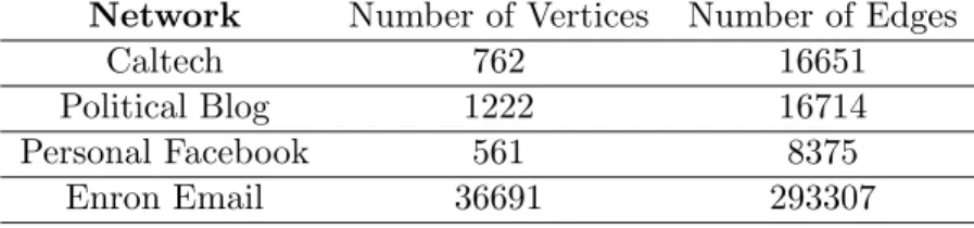
We first applied ESSC to four real networks of various size and density: the Caltech Facebook network (Traud et al., 2011), the political blog network (Adamic and Glance, 2005), the personal Facebook network of the first author, and the Enron email network (Leskovec et al., 2009). We summarize the networks in our application study in Table 3.2
evaluate the ability of each method to capture specific features of these two complex networks through a formal classification study. All methods were run on a 4 GB RAM, 2.8 GHz dual processor personal computer.
Network Number of Vertices Number of Edges
Caltech 762 16651
Political Blog 1222 16714
Personal Facebook 561 8375
Enron Email 36691 293307
Table 3.2: Summary statistics of the four networks that we analyze.
3.4.1 Caltech Facebook Network
The Caltech Facebook network of Traud et al. (2011) represents the friendship relations of a group of undergraduate students at the California Institute of Technology on a single day in September, 2005. An edge is present between two individuals if they are friends on Facebook. In addition to friendship relations, several demographic features are available for each student, including dormitory residence, college major, year of entry, high school, and gender. A summary of these features is given in Table 3.3. This data set provides a natural benchmark for community detection methods due to the possible association of community structure with one or more demographic features. Previous studies have found that this network displays community structure closely matching the dormitory residence of the individuals (Traud et al., 2011).
Feature k pm m M
Dormitory 8 0.2205 44 98
Year 15 0.1457 1 173
Major 30 0.0984 1 88
High School 498 0.1693 1 3
Gender 2 0.0827 227 472
Table 3.3: A summary of the features associated with the individuals in the Caltech Facebook network. From left to right, kis the number of unique categories, pm is the proportion of missing
3.4.1.1 Quantitative Comparison
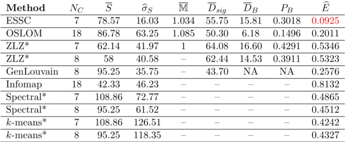
We first compare the communities detected by each method based on quantitative summaries of the communities themselves: the number and size of the communities; the overlap present; and the number of background vertices found. A summary of the findings is given in Table 3.4. ESSC took 1.584 seconds to run on this network.
Method NC S σbS M Dsig DB PB Eb
ESSC 7 78.57 16.03 1.034 55.75 15.81 0.3018 0.0925
OSLOM 18 86.78 63.25 1.085 50.30 6.18 0.1496 0.2011
ZLZ* 7 62.14 41.97 1 64.08 16.60 0.4291 0.5346
ZLZ* 8 58 40.58 – 62.44 14.53 0.3911 0.5323
GenLouvain 8 95.25 35.75 – 43.70 NA NA 0.2576
Infomap 18 42.33 46.23 – – – – 0.8132
Spectral* 7 108.86 72.77 – – – – 0.4865
Spectral* 8 95.25 61.52 – – – – 0.4512
k-means* 7 108.86 126.51 – – – – 0.4242 k-means* 8 95.25 118.35 – – – – 0.4327
Table 3.4: A summary of the detection methods run on the Caltech Facebook network. From left to right, NC is the number of communities detected, S is the average size of the communities, bσS
is the standard deviation of the community size,M is the average number of communities to which
non-background vertices belong, Dsig is the average degree of the vertices in a community,DB is
the average degree of the background vertices,PB is the proportion of background vertices and Eb
is the mean classification error associated with the dormitory feature of the individuals. *Methods were set to find 7 and 8 communities, based on the number of communities detected by ESSC and GenLouvain. – : represents repeated values.
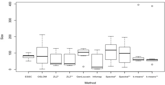
We note that the ZLZ,k-means, and Spectral methods require prior specification of the num-ber of discovered communities. Based on the ESSC and GenLouvain results, we ran each of these methods with seven and eight detected communities. We show the size distributions of the detected communities for each method in Figure 3.1, and find that the size distribution is broadly similar across the ESSC, ZLZ, Genlouvain, and Spectral methods. Infomap found many (NC=18) small
0
100
200
300
400
Method
Si
ze
ESSC OSLOM ZLZ* ZLZ** GenLouvain Infomap Spectral* Spectral** k-means* k-means**
Figure 3.1: The size distributions of communities from each detection method when run on the Caltech network.
from 1 to 1.085. Each of the methods capable of detecting background (ESSC, OSLOM, and ZLZ) designated more than 15% of the total network as background, and vertices contained within communities had average degree nearly three times that of background vertices. This suggests, as expected, that the background vertices are less connected to other vertices in the network.
3.4.1.2 Community Features
demographic features as a discrete response that we wish to predict. We describe our approach in more detail.
Suppose that a detection method divides the vertices of the network into K communities plus background. Then then×K matrixX= [xi,j] defined by
xi,j =
1 if vertexi belongs to communityj 0 otherwise
represents the detected community structure of the network. For a given demographic feature α takingL values, letyiα∈[L] be the value of α in sample i. We ignore samples for which the value of feature α is not available. Treating the i’th row of the matrix X as a K-variate predictor for yiα, we use the Adaboost classification method (Freund and Schapire, 1995) with tree classifiers to construct a prediction rule φ:{0,1}K →[L].
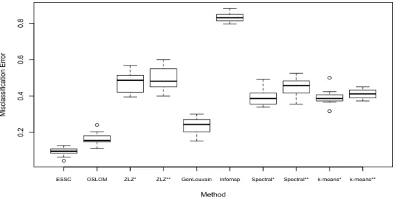
To evaluate each method, we first randomly divide the n samples into ten equally-sized sub-groups. Then by setting aside one subgroups as a test set, we train the classifier on the remaining subgroups and predict the features of the test set. By subsequently treating each subgroup as a test set in this way, we calculate the misclassification error associated with each test. We report the average misclassification error Eb for each method as a means of comparison and report the results
in Table 3.4. The distribution of errors are shown in Figure 3.2. Values of Eb near zero suggest
that the detected community structure captures the clustering of the selected feature. We consider the dormitory residence of the network as this feature has been shown to be most representative of the community structure in past studies (Traud et al., 2012). From Figure 3.2, we see that ESSC has the lowest misclassification error among competing methods in this classification study. These results suggest that the detected communities of ESSC best match the dormitory residence of the Caltech network.
3.4.2 Political Blog Network
0.2
0.4
0.6
0.8
Method
Mi
scl
assi
fica
tio
n
Erro
r
ESSC OSLOM ZLZ* ZLZ** GenLouvain Infomap Spectral* Spectral** k-means* k-means**
Figure 3.2: The misclassification error of each method based on the ten-fold classification study performed on the Caltech network. The community containment of each individual was used to classify his/her dormitory residence. For each test, an Adaboost classifier was used for comparison.
affiliation by the authors in Adamic and Glance (2005). These authors, as well as those of Newman (2006b), observed that blogs of a similar political affiliation tend to link to one another much more often than to blogs of the opposite affiliation.
Method NC S σbS M Dsig DB PB Eb
ESSC 2 448.50 75.66 1 36.322 2.577 0.2651 0.0201
OSLOM 11 87.58 79.48 1.110 33.749 5.342 0.225 0.0306
ZLZ** 10 60.00 37.69 1 35.50 2.50 .506 0.1341
GenLouvain 2 611.00 72.12 – 27.36 NA 0 0.0475
Infomap 36 33.94 125.74 – – – – 0.0532
Spectral* 2 611.00 858.43 – – – – 0.3821
k-means* 2 611.00 613.77 – – – – 0.2856
3.4.2.1 Quantitative Comparison:
We first compare the communities detected by each method based on their quantitative character-istics. The results are summarized in Table 3.5. ESSC took 2.012 seconds to run on this network. Both the ESSC algorithm and GenLouvain found two large communities of similar size. In-terestingly, Infomap found thirty-six communities, thirty-four of which contained fewer than 25 vertices. Roughly 95% of the vertices in these smaller communities of Infomap were contained in the background vertices of ESSC. Neither ESSC nor OSLOM found significant overlap among the communities, reflecting the tendency of the political bloggers to communicate with like-minded individuals: as noted by the authors of Adamic and Glance (2005), “divided they blog”.
ESSC, OSLOM, and ZLZ each assigned over twenty percent of the vertices to background. The pairwise Jaccard score of these background sets is greater than 0.67 in each case. The background vertices of all three extraction methods had mean degree six times smaller than vertices within communities, suggesting the presence of sparsely connected background vertices in this network.
3.4.2.2 Political Affiliation:
We now evaluate the extent to which the political affiliation of the blogs “cluster” by conducting the same classification study detailed in Section 3.4.1.2. We report the mean proportion of misclassified labelsEb in Table 3.5. ESSC, OSLOM, Genlouvain, and Infomap all maintained classification errors
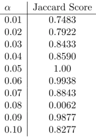
below 10% suggesting that political affiliation is captured by the network’s community structure quite well. ESSC had the lowest misclassification error in this study keeping an error below 4% across all tests. We look deeper into the strength of connection of the background vertices to the true political affiliations. Interestingly, these vertices were still preferentially attached to their true affiliation; however, their associated p-values were typically greater than 0.10 indicating weak affiliation.
3.4.3 Personal Facebook Network
Figure 3.3: A visualization of my personal facebook network. Nodes represent friends of mine on Facebook and edges between nodes represent mutual friendships. Nodes are colored according to the location where I first met each individual.
The understanding of human social interactions has been improved through the analysis of large available social networks like Facebook (Lee and Cunningham, 2013; Traud et al., 2011, 2012). Typically, these networks capture the social activity of individuals of a single location. For example, the Facebook network analyzed in Section 3.4.1 reflects the friendships of individuals specifically from the California Institute of Technology. The personal Facebook network provides one view of how individuals from different schools and locations interact given that they all have one friend in common.
We ran ESSC on the network (running time about 1 second) and found 7 communities with sizes varying from 10 to 157, see Table 3.6. Approximately 18% of the nodes in the network were distinguished as background. The mean degree of the vertices belonging to a community (Dsig ≈ 33) was about seven times that of the background (DB ≈ 5). Of the vertices that were
contained in a community, the average membership was very close to 1, suggesting little overlap between communities.
each case. Groups A, B, C and D represent the schools that the author attended from high school to final graduate school and make up nearly 81% of the total network. Groups E and F are not captured well by the communities; however, this is expected due to the small size of these locations (n = 3 in both cases). Finally, the most highly represented group among the background distinguished by ESSC were acquaintances - individuals met through other friends, events, or conferences. These results suggest that friendships in this network cluster based on location and that the acquaintances of the author are not well connected to his remaining friends.
True Features ESSC Results
Label Size Community Size
Aquaintance 80 1 43
A 62 2 107
B 94 3 75
C 150 4 157
D 147 5 53
E 3 6 26
F 3 7 10
G 22 Background 101 (18.0 %)
Table 3.6: Features of the Personal Facebook Network as well as the results of ESSC. On the left, we list the labels of the individuals according to location, and the size of each group. On the right, we list the detected communities and background as well as their corresponding size.
3.4.4 Enron Email Network
The Enron email network from Leskovec et al. (2009) is a large (36691 vertices), sparse network in which each vertex represents a unique email address. An undirected edge connects any two addresses if at least one email message has been sent from one address to the other. At least one vertex of each edge corresponds to the email address of an employee of the Enron corporation. We ran ESSC on the network with α = 0.05. ESSC took approximately 10 minutes to run on this network.
of background vertices - nearly 83% (30454 vertices) of the network. The average degree of the vertices within a community is nearly twelve times that of the background vertices. ESSC found 8 communities with average size of 1239 and standard deviation 450. The average membership of the vertices that were contained within a community was 1.409 indicating a moderate amount of overlap of communities.
3.5 Simulation Study
In this section we evaluate the performance of ESSC on simulated networks with three primary types of community structure: 1) communities that partition the network; 2) communities that overlap and cover the network; and 3) disjoint communities plus background.
Networks of the first two types have been well-studied, and there are several existing simulation benchmarks for these structures (Girvan and Newman, 2002; Lancichinetti and Fortunato, 2009a,b). We make use of the Lancichinetti, Fortunato, and Radicchi (LFR) benchmark from Lancichinetti and Fortunato (2009a,b) in order to assess the performance of ESSC and other methods on networks of the first two types. Our principal reason for using the LFR simulation benchmark is its flexibility, as well as the fact that the power-law degree distribution it employs is representative of the degree heterogeneity present in many real networks (Barab´asi and Albert, 1999). ESSC performs well on these standard non-overlapping and overlapping benchmarks, and is in fact competitive with the other detection methods in these settings. We evaluate the results on these benchmarks in Section 3.7.1.
Relatively little attention has been paid to networks with background vertices, and we are not aware of a simulation benchmark for networks of this sort. We therefore propose a flexible simulation benchmark for networks with background that extends the LFR benchmark, and use it to compare ESSC with competing methods.