Development and application of ligand-based and structure-based computational drug discovery tools based on frequent subgraph mining of chemical structures

(1)

DEVELOPMENT AND APPLICATION OF LIGAND-BASED AND STRUCTURE-BASED COMPUTATIONAL DRUG DISCOVERY TOOLS STRUCTURE-BASED ON

FREQUENT SUBGRAPH MINING OF CHEMICAL STRUCTURES

Raed Saeed Khashan

A dissertation submitted to the faculty of the University of North Carolina at Chapel Hill in partial fulfillment of the requirements for the degree of Doctor of Philosophy in the School of Pharmacy (Division of Medicinal Chemistry and Natural Products).

Chapel Hill 2007

Approved by:

Dr. Alexander Tropsha Dr. Weifan Zheng Dr. Alexander Golbraikh Dr. Wei Wang

(2)

(3)

ABSTRACT

RAED KHASHAN: Developmment and Application of Ligand-based and Structure-based Computational Drug Discovery Tools Based on Frequent Subgraph Mining of Chemical

Structures

(Under the direction of Alexander Tropsha)

(4)

This dissertation is dedicated to

my Mother, Father, and all my family members, whose support, encouragement, and personal sacrifice

(5)

ACKNOWLEDGEMENTS

Dr. Alexander Tropsha for his scientific guidance, support and encouragement during my graduate studies.

Dr. Weifan Zheng, for his concern, scientific guidance as well as his advices, especially those related to my future career.

Drs. Alexander Golbraikh, Wei Wang, and Andrew Lee for their time and effort in assisting, and guiding this research project.

Labmates in 301 Beard Hall; Dr. Min Shen, Dr. Scott Oloff, Dr. Shuxiang (King) Zhang, Chrisopher Grulke, Rima Hajjo, and all my labmates for their friendship, support, and scientific discussion over the years.

My former adviser, Professor Robert Pearlman for his valuable advice and guidance in the early stage of developing my research skills.

(6)

TABLE OF CONTENTS

LIST OF TABLES……….………ix

LIST OF FIGURES……….……..…xi

ABBREVIATIONS………..xiii

Chapter I. INTRODUCTION...1

Introduction to Frequent Subgraph Mining ...3

Fast frequent subgraph mining (FFSM) algorithm ...4

Overview of Chapter 2...7

II. DEVELOPMENT OF FRAGMENT-BASED CHEMICAL DESCRIPTORS ...10

Introduction...10

Computational Methods...13

Application of FFSM to chemical datasets to generate chemical fragment descriptors...13

Removing redundant chemical fragments ...17

Experimental datasets ...20

(7)

Generating the fragment-based chemical descriptors ...28

Building kNN-classification models...32

Comparison with other molecular descriptors ...35

Conclusions...38

III. DENTIFYING TWO-DIMENSIONAL (TOPOLOGICAL) PHARMACOPHORES/TOXICOPHORES ...39

Introduction...39

Application of FFSM to chemical datasets to generate closed subgraphs and use them as chemical fragments ...41

Classification based on association (CBA) method...43

Experimental datasets ...47

Method validation ...48

Results and Discussion ...51

Examples of associated fragments for the Ames Mutagenicity dataset...55

Examples of associated fragments for the MRTD dataset...64

Examples of associated fragments for the PGP dataset ...77

Weaknesses and strengths of the descriptors and methodology ...86

Conclusions...86

IV. DEVELOPMENT OF POSE-SCORING FUNCTION FOR PROTEIN-LIGAND BINDING BASED ON FREQUENT PATTERNS OF INTER-ATOMIC INTERACTIONS AT THEIR INTERFACES...88

(8)

Dataset of Protein-Ligand Complexes ...92

Graph Representation of the Protein-Ligand Interface...93

Application of Frequent Subgraph Mining to Identifying Frequent Atomic Interaction Patterns at the Protein-Ligand Interface. ...96

Deriving the Scoring Function Using Frequent Protein-Ligand Interaction Patterns...99

Validation of the Scoring Function...100

Results and Discussions...104

Identification of “classical” interaction patterns in the internal training set and external test set scoring. ...104

Applying more stringent external test: switching the internal training and external test sets. ...113

Conclusions...117

Acknowledgments...119

V. SUMMARY AND FUTURE DIRECTIONS...120

Summary and Future Directions of Chapter 2 ...122

(9)

LIST OF TABLES Table

3.1 Internal dataset for Salmonella, has a prediction a total error of 19.6% using the fingerprints descriptors...44 3.2 External validation for Salmonella, has a total error of 28.2% using

fingerprints descriptors. ...44 3.3 Internal dataset for Salmonella, has a prediction a total error of 14.6%

using the fragment-based chemical descriptors. ...46 3.4 External validation for Salmonella, has a total error of 22.0% using

fragment-based chemical descriptors...46 3.5 Example of rules used in the classifier built by CBA...48 3.6 Internal dataset for MRTD, has a prediction a total error of 11.7% using

the fingerprints descriptors. ...54 3.7 External validation for MRTD, has a total error of 28.1% using

fingerprints descriptors. ...54 3.8 Internal dataset for MRTD, has a prediction a total error of 8.2% using

the fragment-based chemical descriptors...55 3.9 External validation for MRTD, has a total error of 26.2% using

fragment-based chemical descriptors...55 3.10 Example of rules used in the classifier built by CBA...57 3.11 Internal dataset for PGP, has a prediction a total error of 1.5% using the

fingerprints descriptors. ...65 3.12 External validation for PGP, has a total error of 30.2% using fingerprints

descriptors...65 3.13 Internal dataset for PGP, has a prediction a total error of 3.8% using the

fragment-based chemical descriptors...66 3.14 External validation for PGP, has a total error of 23.8% using

(10)

3.15 Internal dataset for PGP, has a prediction a total error of 3.0% using the fragment-based chemical descriptors derived from the whole PGP dataset. ...68 3.16 External validation for PGP, has a total error of 17.7% using

fragment-based chemical descriptors derived from the whole dataset...68 3.17 Example of rules used in the classifier built by CBA...70 3.18 Internal dataset for PGP, has a total error of 13.6% using the

fragment-based chemical descriptors. ...75 3.19 External validation for PGP, has a total error of 27.0% using

fragment-based chemical descriptors and simple rules built by CBA...75 3.20 External validation for PGP, has a total error of 23.8% using

fragment-based chemical descriptors and closed rules in place of the simple rules built by CBA. ...75 3.21 Screening Maybridge database seeded with the external dataset of PGP

gave a total error of 14.3% using fragment-based chemical descriptors and simple rules built by CBA...77 3.22 Screening Maybridge database seeded with the external dataset of PGP

(11)

LIST OF FIGURES Figure

1.1 Top: Examples of three labeled graphs (referred to as a graph database). The labels of the nodes are specified within the circle and the labels of the edges are specified along the edge. The mapping q1 → p2, q2 → p1, q3→ p3 represents an induced subgraph isomorphism from graph Q to P. Bottom: All the frequent induced subgraphs with support ≥ 2/3 for the

graph database...6

2.1 Conversion of each molecule in the dataset into undirected, labeled graph...14

2.2 Using FFSM to find common subgraphs in at least a subset of molecules of size 2 out of 3 molecules (σ = 2/3) ...15

2.3 Matrix of counts (number of occurences) for each subgraph (chemical fragments) in each molecule in the dataset. ...16

2.4 Matrix of counts (number of occurences) for closed subgraphs (chemical fragments) in each molecule in the dataset. ...19

2.5 kNN QSAR modeling approach (a) and predictive QSAR modeling workflow (b). ...27

2.6 Number of subgraphs as a function of the support value (% σ). ...29

2.7 Distribution of the size (number of nodes) of the subgraphs using support value σ = 1% before and after removing redundant subgraphs. ...31

2.8 Model fitness as a function of support σ (%) for PGP...33

2.9 Model fitness as a function of support σ (%) for MRTD. ...33

2.10 Model fitness as a function of support σ (%) for Ames genotoxicity...34

2.11 External sets prediction accuracies for each dataset. ...34

2.12 External sets prediction accuracies for each dataset using fragment-based and MolConnZ descriptors. ...37

(12)

3.2 Matrix of 1’s and 0’s for the occurrence or not, respectively, of the closed subgraphs (chemical fragments) in each molecule in the dataset, as well as the class label for the molecule...45 3.3 Work flow for the division of the datasets; identifying chemical fragments;

generation of class association rules; and external validation. ...50 4.1 Inter-atomic interactions at the protein-ligand interface, within a distance

cutoff 3.15 A°. Protein is “adenosine deaminase”, and ligand is “PRH“ in the “1a4m” PDB complex...95 4.2 Example of 4 different geometries for an interaction pattern between

protein and ligand atoms as well as water molecules. ...98 4.3 Work flow for the validation of the method. ...103 4.4 Comparison between scoring functions using 231 (core set) as external

testing set, and the remaining 860 as internal training set. ...106 4.5 The number of protein complexes in the external test set as a function of

the rank order of the native pose for these complexes...108 4.6 The number of protein complexes in the external test set as a function of

the rank order of the pose with the smallest RMSD for these complexes. ...110 4.7 Rank order as function of RMSD for the protein-ligand complex ”1nc3”. ...112 4.8 Comparison between scoring functions using 231 (core set) as internal

training set, and the remaining 860 as external test set...114 4.9 Comparison between scoring functions using 860 complexes as internal

(13)

ABBREVIATIONS

2D Two dimensional.

3D Three dimensional

AUC Area under the curve.

CADD Computer-assisted drug design. CARs Class Association Rules.

CBA Classification based on association. CCR Correct Classification Rate.

FFSM Fast frequent subgraph mining. FP-tree Frequent patterns tree.

ILP Inductive logic programming. ISIDA In silico design and data analysis. kNN k-Nearest Neighbors.

LOO Leave one out. MoAD Mother of All Databases.

MRTD Maximum Recommended Therapeutic Dose. PDB Protein Data Bank.

PGP P-Glycoprotein.

QSAR Quantitative structure-activity relationship. QSPR Quantitative structure-property relationship. RMSD Root mean square deviation.

(14)

CHAPTER 1 INTRODUCTION

(15)

and the sub-graph mining approach, as we shall explain later. The medicinal chemist can easily interpret these descriptors. In addition, new important fragments that might have not been defined a priori can be discovered. The research question that needs to be answered in the course of this project is whether these descriptors can indeed give a better predictive QSAR model as compared to those generated with current descriptors.

A popular ligand-based drug design method is the so-called Active Analog Approach (Sheridan, R., Rusinko, A., Nilakantan, R., Venkataraghavan, R., 1989). It is used to explore active compounds that bind to same target protein in order to identify “pharmacophoric” groups responsible for the specific activity; these groups are subsequently used to screen chemical databases for new leads. In this project, we will answer the question whether the frequent sub-structures can be used as novel means to identify the pharmacophoric groups and then examine their ability to identify new leads in the context of the Active Analog Approach. The significance of this particular study rests on the fast identification of the pharmacophoric groups for database mining. The advantage of our proposed approach is that it does not rely on 3D conformational search of the structures and therefore it is highly efficient computationally.

(16)

ultimately do not succeed if they do not differentiate correct poses from incorrect ones, and if “true” ligands can not be identified. So, the design of reliable scoring functions and protocols is of fundamental significance.

With the exponential increase in the number of protein-ligand crystal structures in the protein databank (PDB), researchers are more interested in exploring the information that can be gathered from these structures. This project will try to answer the question whether the frequent patterns of inter-atomic interactions at the protein-ligand interface can be used in forming new more precise scoring functions and docking schemes as compared to current methods. The study can be highly significant and of interest to many researchers in that field. The study will also bring insights to the structure based de novo design of ligands complementary to the active sites.

INTRODUCTION TO FREQUENT SUBGRAPH MINING

(17)

Given a set S of graphs, frequent subgraphs that occur in a fraction (support value) of all graphs S are found. For any frequent subgraph mining algorithm, there are two computationally challenging problems: First, subgraph isomorphism, which is determining whether a given graph is a subgraph of another graph. Second, enumerating all frequent subgraphs efficiently (Huan et al, 2003). There are several efficient subgraph mining algorithms that have been presented in a recent review by Huan et al, 2003. For our study, we have been using Fast Frequent Subgraph Mining (FFSM) algorithm which will be described in the following section. The FFSM algorithm will be applied to mine datasets of small molecules to find frequent patterns (chemical fragments) that can be used for classification purposes as we will see in Chapter 2 and Chapter 3. In addition, it will be applied to find frequent paterns of interactions at the protein-ligand complexes as we will see in Chapter 4. Fast frequent subgraph mining (FFSM) algorithm

The FFSM algorithm was developed by our collaborators in the Computer Science Department as a general highly efficient tool to find common frequent subgraphs in a family of labeled unidirectional graphs. A labeled graph G is defined as a five element tuple G = {V, E, ∑v, ∑E, δ} where V is the set of nodes of G and E ⊆ V ×V is the set of

undirected edges of G. ∑v and ∑E are a set of labels and the labeling function δ: V →∑v ∪

E →∑Emaps nodes and edges in G to their labels. The same label may appear on multiple

nodes or on multiple edges, but we require that the set of edge labels and the set of node labels are disjoint.

A labeled graph G = (V, E, ∑v, ∑E, δ) is isomorphic to another graph G'=(V', E', ∑v',

∑E', δ') if and only if there is a bijection f: V → V' such that:

∀ u ∈ V, δ (u) = δ'(f(u)), and

(18)

The bijection f denotes an isomorphism between G and G'.

A labeled graph G= (V, E, ∑v, ∑E, δ) is an induced subgraph of graph G'=(V', E',

∑v', ∑E', δ') if and only if G is subgraph isomorphic to G’ and preserves all G’ edges

connecting nodes in G.

A labeled graph G is induced subgraph isomorphic to a labeled graph G', denoted by G ⊆ G', if and only if there exists an induced subgraph G'' of G' such that G is isomorphic to G''. Examples of labeled graphs, induced subgraph isomorphism, and frequent induced subgraphs are presented in Figure 1.1.

Given a set of graphs GD (referred to as a graph database, e.g., a database of molecular graphs, the support of a graph G, denoted by supG is defined as the fraction of

graphs in GD which embeds the subgraph G. Given a threshold σ (0 < σ≤1) (denoted as

minSupport), we define G to be frequent, iff supG is at least σ. All the frequent induced

(19)

p2 p5 a b b d y x y y y (P) p1

p3 p4

c a b b y x y (Q) q1 q₃ q2 a b b y y (S) s1 s₃ s2

a b a y b b x b _a

b

y x y

p2 p5

a b b d y x y y y (P) p1

p3 p4

c p2 p5

a b b d y x y y y (P) p1

p3 p4

c a b b y x y (Q) q1 q₃ q2 a b b y y (S) s1 s₃ s2 a b b y x y (Q) q1 q₃ q2 a b b y y (S) s1 s₃ s2

a b a y b b x b _a

b

y x y

a b a y b b x b _a

b

y x y

Figure 1.1. Top: Examples of three labeled graphs (referred to as a graph database). The labels of the nodes are specified within the circle and the labels of

the edges are specified along the edge. The mapping q1 → p2, q2 → p1, q3→ p3

represents an induced subgraph isomorphism from graph Q to P. Bottom: All the

(20)

OVERVIEW OF CHAPTER 2

In this chapter, we present a novel approach to generating fragment-based molecular descriptors. Using labeled chemical graph representation of molecules, Fast Frequent Subgraph Mining (FFSM) method developed in this group is used to find chemical fragments that occur in at least a subset of molecules in a dataset. The counts of frequent fragments have been used as descriptors in variable selection k Nearest Neighbor (kNN) QSAR modeling. This approach was applied to Maximum Recommended Therapeutic Dose (MRTD), Salmonella Mutagenicity (Ames Genotoxicity), and P-Glycoprotein (PGP) datasets. We followed established protocols for model validation, i.e., randomization of target property and splitting the datasets into training, test, and validation sets. Highly predictive models have been generated with the accuracies for the training and test sets exceeding 0.75, and the accuracy for the external validation sets exceeding 0.72. The accuracy results were comparable to commonly used molecular descriptors and in some cases was better. In addition, fragment-based descriptors implicated in validated models can afford mechanistic interpretation of the results in terms of essential pharmacophoric or toxicophoric elements responsible for the compounds’ target property. For interpretation purposes, another classification method will be used as we will see in Chapter 3.

(21)

molecules in a dataset. These chemical fragments are used as binary descriptors for the dataset. Then, Classification-Based Association (CBA) algorithm is used to identify associated chemical fragments responsible for the activity as well as the toxicity (mutagenicity) for datasets of compounds and provide interpretation for these results. The method is validated for its ability to predict the activity/toxicity of an external dataset. This approach was applied to a dataset of P-Glycoprotein substrates (PGP), Maximum recommended therapeutic dose dataset (MRTD), and to a dataset of mutagenic compounds (Salmonella Ames Mutagenicity dataset). The prediction ability of the method using the chemical fragments identified was compared to that when using Fingerprints descriptors. The results show a significant improvement in the predictive ability when using the chemical fragments identified in this method over the Fingerprints descriptors.

(22)

(23)

CHAPTER 2

DEVELOPMENT OF FRAGMENT-BASED CHEMICAL DESCRIPTORS

INTRODUCTION

QSAR modeling is fundamentally based on the similarity principle implying that similar compounds have similar biological properties. Consequently one can predict the biological target property of a molecule from that of chemically similar compounds for which the property is known. To build quantitative predictive models a similarity metric is required; therefore a unit of measurement such as molecular descriptors needs to be identified. Once the descriptors are defined, QSAR techniques can be used to relate the chemical structure of a molecule to its target property.

(24)

descriptors could potentially provide a mechanistic explanation of the dependence of the target property on molecular structure. Such explanation especially with respect to the differences between active and inactive molecules could provide useful guidance to medicinal chemists with respect to rational design of new biologically active chemical entities.

(25)

Finding patterns from graphs has long been an interesting topic in the data mining/machine learning community. For instance, Inductive Logic Programming (ILP) has been widely used to find patterns from graph dataset (Dehaspe, Toivonen, and King, 1999). However, ILP is not designed for large databases. Other pioneer methods focused on approximation techniques such as SUBDUE (Holder, Cook, and Djoko, 1994) or on heuristics such as the greed based algorithm (Yoshida and Motoda, 1995). Several algorithms have been recently developed by the data mining community to solve the so-called frequent subgraph mining problem which reports all frequent subgraphs of a group of general graphs (Huan, Prins, and Wang, 2003; Huan et al., 2004; Kuramochi and Karypis, 2001;Yan and Han, 2002). These techniques have been successfully applied in cheminformatics where compounds are modeled by undirected graphs. Recurring substructures in a group of chemicals with similar activity are identified by finding frequent subgraphs in their related graphical representations. The recurring substructures can implicate chemical features responsible for compounds’ biological activities (Deshpande, Kuramochi, Wale, and Karypis, 2005).

Our fragment-based descriptors are derived based on frequent common substructures that are found in at least a subset of molecules (this fraction is defined as a

(26)

(a) provide a detailed description of the frequent subgraph mining approach as applied towards developing the fragment-based descriptors; (b) validate these descriptors by developing predictive QSAR models (using k-Nearest Neighbor (kNN) QSAR techniques) for several experimental datasets, and (c) finally, discuss the applications of these descriptors in the QSAR analysis for drug design and development.

COMPUTATIONAL METHODS

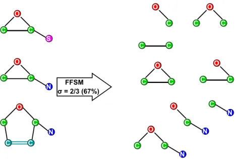
Application of FFSM to chemical datasets to generate chemical fragment descriptors. The molecules are described in the SYBYL MOL2 file format, which considers 33 atom types and 5 bond types. Chemical structures are then represented as hydrogen suppressed graphs, where atoms are considered as labeled nodes and bonds are labeled edges. Then, the FFSM algorithm described earlier in Chapter 1 is used to find the frequent (chemical) subgraphs for a given a support value (σ), which is one of the model variables defined by the user. Figure 2.1 shows an example for representing three molecules comprising a small dataset as labeled unidirectional graphs and Figure 2.2 presents a simple example of the output generated as a result of applying FFSM to this small dataset with the support value of 66.7% (i.e. σ = 2/3).

(27)

O

H₂C CH SH

O

H₂C CH

NH₂

O

H₂C CH NH2

C C

O

C C

S

O

C C

N

O

C C

N

C C

Chemical Graphs

(28)

O C C N O C C N C C O C C C O C C O C C O C C O C C N C N O C N FFSM

σ= 2/3 (67%) O

C C

S

Figure 2.2 Using FFSM to find common subgraphs in at least a subset of

(29)

O C C O C C O C C O C O C C O

H2C CH

NH2

C C O

H2C CH

NH2

O

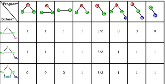
H2C CH SH C N O C N O C C N 1 1 1 3/2 1 0 0 0 1 1 1 3/2 1 1 1 1 0 0 0 3/2 1 1 1 1 Fragment Dataset

(30)

Removing redundant chemical fragments

The application of the FFSM algorithm to chemical datasets may result in the identification of redundant features. For example, if an aromatic group is found to be frequent, then all the sub-structures within such aromatic group will also be frequent in spite of having any of these sub-structures present independently in the molecular dataset. This problem of subgraph redundancy is well known in graph mining, and the resulting subgraphs after removing redundant ones are called closed subgraphs. A subgraph g is closed in a database if there exist no proper supergraph of g that has the same support as g (Yan, X., and Han, J., 2003). In our studies reported herein to eliminate the redundancy in the frequent subgraphs (chemical fragments) leaving only closed ones, the following criteria was used:

For each two frequent subgraphs SGi and SGj: If (SGi ⊆ SGj) and

support (SGi) = support (SGj), then remove SGi.

However, a subgraph SGi that is embedded in SGj (i.e. SGi ⊆ SGj) and has the same support value as SGj will not be deleted if it also occurs by itself (not as part of the SGj) in the graph database of molecules. This is important since it will retain subgraphs that can be useful.

(31)

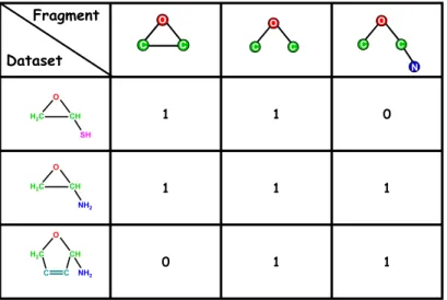
two subgraph descriptors. Therefore, for our toy example we will end up with only three closed subgraphs that will be used as our unique descriptors (see Figure 2.4).

(32)

O

C C

O

C C

O

H2C CH

NH2

C C O

H2C CH

NH2

O

H2C CH SH

O

C C

N

1 1

0

1 1

1

0 1

1

Fragment

Dataset

(33)

Experimental datasets

Three datasets were used in this study. The first one included 1217 drug-like molecules with the MRTD (Maximum Recommended Therapeutic Dose) as their target property. This dataset was recently analyzed by the FDA modeling group (Contrera et al., 2004). Following the approach described in the original publication all molecules were divided into two classes based on the MRTD cutoff value. This results in having 576 molecules with toxicological effect (adverse or undesirable pharmacological effect), and 641 molecules without toxicological effect. The second dataset is composed of 3434 drug-like molecules with the Salmonella mutagenic activity score as the target property. The score ranged from 10 to 80; molecules with no mutagenic activity have a score of 10, and the most mutagenic molecules have a score of 80. A cutoff value is used to divide the dataset into 2 classes: mutagenic and non-mutagenic, and thus resulting in 1615 mutagenic molecule versus 1819 non-mutagenic molecules. This dataset was described in a paper by Votano et al., 2004. The third dataset included 195 molecules shown to be substrates (108 molecules) or non-substrates (87 molecules) of the P-Glycoprotein Protein (PGP). This dataset was analyzed previously in our group using several modeling techniques and descriptor sets and its molecules were taken from a paper by Penzotti et al., 2002. Thus, all experimental datasets have a binary value as their target property.

QSAR model development and validation methods

(34)

previous studies in this as well as several other laboratories demonstrated that no correlation exists between leave-one-out (LOO) cross-validated R2 (q2) for the training set and the correlation coefficient R2 between the predicted and observed activities for the test set(Golbraikh and Tropsha, 2002; Kubinyi, Hamprecht, and Mietzner, 1998). These findings indicated that in order to obtain QSAR models with high predictive ability, external validation was critical. Thus, each dataset of compounds was divided randomly into external and internal sets. Then, the internal set was divided into multiple chemically diverse training and test sets with a rational approach implemented in our group(Golbraikh and Tropsha, 2002) based on the Sphere Exclusion (SE) algorithm(Snarey et al., 1997). SE is a general procedure that is typically applied to molecules characterized by multiple descriptors of their chemical structures. The entire dataset can then be treated as a collection of points (each point corresponding to an individual compound) in the multidmensional descriptor space. The goal of the SE method is to divide a dataset into two subsets (training and test sets) using a diversity sampling procedure(Golbraikh and Tropsha, 2002).

The SE algorithm used in this study included the following steps. The algorithm starts with the calculation of the distance matrix D between points representing compounds in the multidimensional descriptor space. Let Dmin and Dmax be the minimum and

maximum elements of D, respectively. N probe sphere radii are defined by the following formulas: Rmin=R1=Dmin, Rmax=RN=Dmax/4, Ri=R1+(i-1)*(RN-R1)/(N-1), where i=2, …, N-1.

(35)

probe sphere around this point. (iv) Select points from this sphere and include them alternatively into test and training sets. (v) Exclude all points within this sphere from further consideration. (vi) If no more compounds left, stop. Otherwise let m be the number of probe spheres constructed and n be the number of remaining points. Let dij

(i=1,…,m; j=1,…,n) be the distances between the remaining points and probe sphere centers. Select a point corresponding to the lowest dij value and go to step (ii). The training

sets were used to build models and the test sets were used for model validation.

Correct classification rate (CCR). Typically, CCR is defined as the ratio of compounds classified correctly to the total number of compounds. This definition of CCR has a major drawback, if the counts of compounds belonging to different classes are significantly different. Suppose there are two classes, class 1 contains 75 compounds and class 0 contains 23 compounds. Assume that some hypothetical "model" will assign all compounds to class 1. Then CCR=0.76, since 75/(75+23)=0.76, i.e. we would believe that our "model" is very good contrary to the common sense.

To avoid artificial overrating of the classification model accuracy, in this study CCR was defined as follows. Let N be the total number of compounds in a dataset, and N1

and N0 be the number of compounds in class 1 and the number of compounds in class 0,

respectively (i.e., N0+N1=N). Let T1 and T0 be the number of compounds predicted as

class 1 and the number of compounds predicted as class 0, respectively. Then

CCR=0.5(T1/N1+T0/N0). (1)

(36)

kNN-Classification. The stochastic variable selection kNN classification method is based on the idea that assigning a compound to a class can be defined by the class membership of its nearest neighbors (in a multi-dimensional chemistry space) taking into account weighted similarities between a compound and its nearest neighbors as follows (see Figure 2.5). Let N be the number of compounds in a dataset. In the simplest case of binary classification, these compounds are distributed between classes a or b. Let na and nb

be the number of compounds in classes a and b, respectively, and m be the number of descriptors (composing the multi-dimensional chemistry space) selected by the variable selection kNN classification procedure. The Tanimoto coefficient can be used as a similarity measure between two classes as follows:

∑

= = = = − + = _m i b i a i m i b i m i a i m i b i a i D D D D D D b a T 1 1 2 1 2 1 ) ( ) ( ) ,

( , (2)

Where a i

D and b i

D are average values of descriptor i for classes a and b, respectively: a n j a ij a i n D D a

∑

= = 1 and b n j b ij b i n D D b

∑

= = 1 ,

Where a ij

(37)

∑

= = = =                     − − = k p p k q k p ip iq k p ip ip C

i T a C

d d d d S 1

1 '1

' 1 ' ' , ( , ) ) / exp( ) / exp( α α

, (3)

Where a_p in T(a_p,C) is the class of compound p, α is a parameter, which in this study was set to 1, and dip is the distance between compound i and its p-th nearest neighbor.

In the leave-one-out cross-validation procedure, the similarity between compound i and each class C is calculated according to the following expression:

∑

= =             − − = k j C j k j ij ij C i S d d S 1 , 1 ' ' ' , ) exp( ) exp( (4)

Compound i is assigned to the class which corresponds to the highest value of ' ,C i

S . The CCR for the training set (CCRtrain) is calculated using formula (1).

Applicability Domain of kNN QSAR Models. For assigning an external compound (which was not included in the training set) to a class, its representative point in the descriptor space must be not too far from its nearest neighbors of the training set. The similarity threshold was defined as the maximum squared distance between a compound, for which the prediction is made and its nearest neighbors of the training set. This squared distance can be defined as a sum of the average squared distance between nearest neighbors within the training set and a number Z of standard deviations of the squared distances from the average: D2max=<D2near.neighb>+Zσnear.neighb. The threshold is referred to here as Z-cutoff.

(38)

All compounds of the test set are selected, for which the distances to their nearest neighbors in the training set were within the defined Z-cutoff. (3) Similarity of each compound chosen in step (2) to each class is calculated using formula (4). The compound is assigned to a class, to which it has the highest similarity. (4) Classification accuracy of the model is characterized by the CCR for the test set (CCRtest) calculated with the formula

(1). Maximum Z-cutoff value, for which reliable prediction of new compounds can be obtained, is a characteristic of the applicability domain of a QSAR model. In this study, Z-cutoff was set to 1.0.

Classification kNN QSAR is a stochastic variable selection procedure based on the simulated annealing approach. The procedure is aimed at the development of a model with the highest fitness [CCRtrain]. The procedure starts with the random selection of a

predefined number of descriptors out of all descriptors. Compound excluded in LOO CV procedure is assigned to a class corresponding to a highest SiC (see formula (3)), where i is

the number of the excluded compound. After each run, cross-validated CCRtrain is defined

(see formula (1)) and a predefined number of descriptors are randomly changed (mutated). The new value of CCRtrain is obtained using the modified subset of descriptors. If CCRtrain(new) > CCRtrain(old), the new subset of descriptors is accepted. If CCRtrain(new) ≤ CCRtrain(old), the new subset of descriptors is accepted with probability p =

exp(CCRtrain(new) – CCRtrain(old))/T, and rejected with probability (1-p), where T is a

simulated annealing parameter, “temperature”. During the process, T is decreasing until the predefined value. Thus, CCRtrain is optimized. In the prediction process, the final set of

(39)

This implementation is similar to that reported for the continuous kNN QSAR method developed in our laboratory earlier (Zheng, W. and Tropsha, A., 2000).

In all calculations reported in this work, the maximum number of nearest neighbors used (k) was 5, Tmax= 1000, Tmin=10-6, temperature decrement was 0.90, and the number of

(40)

(a)

(b)

Figure 2.5. kNN QSAR modeling approach (a) and predictive QSAR modeling workflow (b).

Only accept models that

have: q2_{> 0.75} R2_{> 0.75} Multiple Training Sets

Validated Predictive Models with High Internal

& External Accuracy Original Dataset Multiple Test Sets kNN QSAR Modeling Split into External, Training, and Test Sets Activity Prediction Y-Randomization External validation using applicability domain Database Screening

Randomly select a subset of MMvvaarr descriptors

Exclude a compound

Find the K nearest neighbors of the excluded compound in the selected subspace of descriptors

Calculate the correct classification rate

Simulated Annealing

M times

Calculate the similarities of the compound to each class. Assign it to the class to which it has the highest similarity

(41)

Comparison with other molecular descriptors. In order to demonstrate that the fragment-based chemical descriptors perform just as good as the other molecular descriptors, we compare it with the commonly used MolConnZ molecular descriptors (Kellogg, G., Kier, L., Gaillard, P., and Hall, L., 1996), and the fingerprints descriptors (as we will see in Chapter 2). Models were built for the same datasets using the same techniques and sets of parameters.

RESULTS AND DISCUSSIONS

There are many parameters that are playing a role in finding models with the best predictive ability. In this section we study these parameters and show how they affect the model development process.

Generating the fragment-based chemical descriptors

(42)

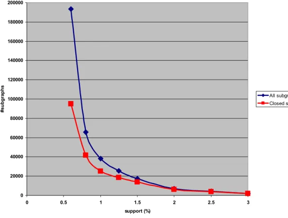
0 20000 40000 60000 80000 100000 120000 140000 160000 180000 200000

0 0.5 1 1.5 2 2.5 3 support (%)

#s

ubgra

phs _{All subgraphs}

Closed subgraphs

(43)

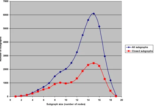
The dark blue line shows the raw number of subgraphs generated by FFSM; the red line shows the number of subgraphs after removing redundant subgraphs leaving only the closed ones (cf. Methods). Notice how the number of subgraphs increases exponentially as thte support value decreases, and notice the large drop in the number of closed subgraphs.

Figure 2.7 shows the size distribution of the subgraphs before and after removing correlated subgraphs for a single support value of 1.0 %. The size of a subgraph is simply the number of nodes in that subgraph.

(44)

0 1000 2000 3000 4000 5000 6000 7000

0 2 4 6 8 10 12 14 16 18 20

Subgraph size (number of nodes)

N

u

m

b

er

of

s

u

bg

ra

ph

s

All subgraphs Closed subgraphs

Figure 2.7. Distribution of the size (number of nodes) of the subgraphs using

(45)

Building kNN-classification models

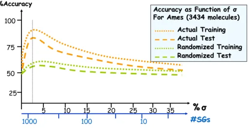
Using the sets of closed subgraphs generated for a range of support values as descriptors classification kNN QSAR was used to build models for the three aforementioned datasets. Figures 2.8-2.10 show the model fitness for each dataset as a function of the support value.

The analysis of the data presented in Figures 2.8-2.10 leads to the following conclusions. The models serve to validate the fragment-based descriptors since high accuracy (>75%) was achieved using actual target property whereas models built with randomized target property gave accuracies <60% (keeping in mind that all three datasets have a binary type target property, meaning that the worst model you can get will have a 50% accuracy).

As the support value increases, the accuracies of models decrease. These observations can be explained easily because smaller number of generic common subgraphs is found and they are not useful in distinguishing between molecules’ target property.

(46)

% %σσ

5 10 15 20 25 30

Actual Training Actual Training Actual Test Actual Test Randomized Training Randomized Training Randomized Test Randomized Test 100 75 50 25 35

Accuracy as Function of Accuracy as Function of σσ

For PGP (195 molecules) For PGP (195 molecules) %Accuracy

%Accuracy

#SGs

10,000 1000 100 10

40 50

1

Figure 2.8. Model fitness as a function of support σ (%) for PGP.

% %σσ

5 10 15 20 25 30

For MRTD (1819 molecules) For MRTD (1819 molecules) %Accuracy

%Accuracy

#SGs

1,000 100 10 1

(47)

% %σσ

5 10 15 20 25 30

For Ames (3434 molecules) For Ames (3434 molecules) %Accuracy

%Accuracy

#SGs

1000 100 10

Figure 2.10. Model fitness as a function of support σ (%) for Ames genotoxicity.

76.79% 72.41% 72.99% 0% 10% 20% 30% 40% 50% 60% 70% 80% 90% 100%

PGP MRTD Ames

P red ic ti o n ac cu ra cy ( % )

(48)

Using the support values that give the best training and test sets’ prediction accuracies for each of the three dataset, and using models with accuracies higher than 75% for both the training and test sets, an external validation prediction was performed. The accuracies for each of the datasets were above 72%, see Figure 2.11.

Comparison with other molecular descriptors

Finally, to compare between descriptors, subgraphs offers a direct interpretation of the features important in determining the target property that is easily understood and utilized by medicinal chemists, as we will address in Chapter 3. In addition, with variable selection kNN, branched features (and disconnected features) are taken care of. Also, since subgraph descriptors are not Boolean descriptors, but counts of subgraphs in the molecule, it should give a better description than structural alert descriptors and fingerprints that are based only on the presence or absence of such sub-structure. In addition to the fact that subgraph descriptors are dataset-derived and not predefined, this will open the door to finding new sub-structures that are not defined apriori.

In this section, we will show the results of comparing the fragment-based descriptors with one of the commonly used molecular descriptors, MolConnZ descriptors. Then in Chapter 3 of the dissertation, we will compare these descriptors with the fingerprints descriptors in terms of their ability to derive accurate predictive models.

(49)

dataset will be compared to that obtained using the MolConnZ molecular descriptors, see Figure 2.12.

(50)

76.79% 72.41% 72.99% 66.92% 72.14% 76.00% 0% 10% 20% 30% 40% 50% 60% 70% 80% 90% 100%

PGP MRTD Ames

P red ic ti o n ac cu racy ( % ) Fragment-based MolConnZ

(51)

CONCLUSIONS

(52)

CHAPTER 3

IDENTIFYING TWO-DIMENSIONAL (TOPOLOGICAL) PHARMACOPHORES/TOXICOPHORES

INTRODUCTION

As discussed earlier in Chapter 2, QSAR modeling is fundamentally based on the similarity principle implying that similar compounds have similar biological properties. Consequently one can predict the biological target property of a molecule from that of chemically similar compounds for which the property is known. To build quantitative predictive models a similarity metric is required; therefore a unit of measurement such as molecular descriptors needs to be identified. Once the descriptors are defined, QSAR techniques can be used to relate the chemical structure of a molecule to its target property.

(53)

in the molecule, fragment-based descriptors could potentially provide a mechanistic explanation of the dependence of the target property on molecular structure. Such explanation especially with respect to the differences between active and inactive molecules could provide useful guidance to medicinal chemists with respect to rational design of new biologically active chemical entities.

Having the ideal descriptors by itself is not enough to do QSAR predictions. The descriptors should be combined with the appropriate modeling technique to provide the best prediction. Based on the nature of the molecular descriptors, one modeling technique might perform better than another. In this study we will describe a unique methodology that is used with the fragment-based descriptors we identify.

(54)

description of the classification method used to utilize these descriptors; (c) validate these descriptors and methodology by developing predictive models for several experimental datasets; (d) compare the descriptors with the commonly used fingerprints descriptors; (e) provide an example of how the models generated can be interpreted to be useful for a medicinal chemist; and (f) finally discuss the applications of these descriptors in the drug design and development process by providing fragments that can be responsible for the target property such as mutagenicity. These examples should be of an interest to many researchers in the field who are concerned about toxicity and safety issues.

COMPUTATIONAL METHODS

Application of FFSM to chemical datasets to generate closed subgraphs and use them as chemical fragments

(55)

O

C C

O

C C

O

H2C CH

NH2

C C O

H2C CH

NH2

O

H2C CH SH

O

C C

N

1 1

0

1 1

1

0 1

1

Fragment

Dataset

(56)

Classification based on association (CBA) method

Classification based on association rules (CBA) is a useful method that can provide an interpretable classification models. The method (described in a paper by Liu, B., Hsu, W., and Ma, Y., 1998) relies on the integration of two powerful data mining techniques: Classification rule mining, which aims to discover a small set of rules in the database to form an accurate classifier (Quinlan, 1992, and Breiman et al., 1984); and Association rule mining which finds all rules in the database that satisfy some minimum support and minimum confidence constraints (Agrawal, and Srikant, 1994).

Let D be the dataset. Let I be the set of all items in D, and Y be the set of class labels. We say that a data case d œ D contains X Œ I, a subset of items, if X Œ d. A class association rule (CAR) is an implication of the form X Ø y, where X Œ I, and y œ Y. A rule X Ø y holds in D with confidence c if c% of cases in D that contain X are labeled with class y. The rule X Ø y has support s in D if s% of the cases in D contain X and are labeled with class y (Liu, B., Hsu, W., and Ma, Y., 1998). In other words:

|| {d œ D | X » y Œ d} ||

Confidence (X Øy) = ___________________ (1) || {d œ D | X Œ d} ||

|| {d œ D | X » y Œ d} ||

Support (X Øy) = ___________________ (2) || D ||

(57)

(58)

O

C C

O

C C

O

H₂C CH

NH2

C C O

H₂C CH

NH₂ O

H2C CH

SH O C C N 1 1 0 1 1 0 1 1 1 0 1 1 Class Fragment Dataset (id)

(a) (b) (c)

(59)

In Figure 3.2, fragments are assigned id’s (a, b, and c) for referral purposes in this example. So, when applying the CBA method to the dataset represented in the figure, the following CARs can be generated:

1. {a} Ø {1}; with 50% confidence, and 33.3% support. 2. {b} Ø {1}; with 66.7% confidence, and 66.7% support. 3. {c} Ø {1}; with 100% confidence, and 66.7% support. 4. {a, b} Ø {1}; with 50% confidence, and 33.3% support. 5. {a, c} Ø {1}; with 100% confidence, and 33.3% support. 6. {b, c} Ø {1}; with 100% confidence, and 66.7% support. 7. {a, b, c} Ø {1}, with 100% confidence, and 33.3% support. 8. {a} Ø {0}; with 50% confidence, and 33.3% support. 9. {b} Ø {0}; with 33.3% confidence, and 33.3% support. 10. {a, b} Ø {0}; with 50% confidence, and 33.3% support.

After that, in building the classifier, the following steps are used. Rules are sorted by their confidence first, then by their support. If two rules have same confidence and support, the one that is generated earlier comes first. Then, for each rule in the sorted sequence, if the rule correctly classifies at least one case, it is marked as a potential rule in the final classifier. Those cases covered by that rule are identified and removed. The total error is computed each time a rule is added, with the default class being the majority class in the data. The process continues until there is no rule or no cases left. Finally, the first rule at which there is the least number of errors recorded is identified as the cutoff rule after which all rules are discarded since they only produce more errors. The undiscarded rules and the default class form the classifier.

(60)

approach is that is to provide the rules with some background items (chemical fragments) that are important for a certain class. These items were not included when building the classifier in CBA because simpler rules come first when rules with equal confidence and support are found. The results of this approach will be compared to those using CBA alone.

Therefore, based on the threshold one uses for the minimum confidence and the minimum support, different classifiers will be built. Then one can decide which one can be accepted as a way to do the external classification for validation of the method. So when classifying a molecule from an external dataset, we look at all the accepted rules in the order they are sorted in the classifier, and see which rule comes first that is applicable to the molecule, and the molecule is classified as having this particular class of that rule, such as mutagenic or non-mutagenic.

Experimental datasets

(61)

molecules. This dataset was described in a paper by Votano et al., 2004. The third dataset included 195 molecules shown to be substrates (108 molecules) or non-substrates (87 molecules) of the P-Glycoprotein Protein (PGP). This dataset was analyzed previously in our group using several modeling techniques and descriptor sets and its molecules were taken from a paper by Penzotti et al., 2002.

Method validation

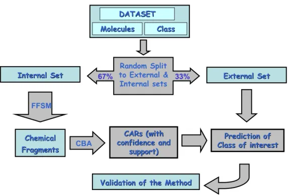
Dataset division into training and external validation sets. As explained earlier in Chapter 2, it is commonly accepted to confirm the validity of the modeling method by dividing the dataset into training and external validation sets (Benigni et al., 2000; Oloff et al., 2006; Trohalaki, Gifford, and Pachter, 2000; Zhang, Golbraikh, and Tropsha, 2006; Zhang et al., 2006). Figure 3.3 explains the work flow for the method development, division of datasets, and validation of the method.

Identifying chemical fragments using FFSM. Using support values in the range 5-10%, closed frequent subgraphs were identified for each dataset and were used as our binary chemical fragments descriptors. Notice that we only look as the presence or absence of a fragment in each molecule in the dataset. This way we can build classification models without having to discretize the values of the descriptors, and then being able to compare it later on with the binary fingerprints descriptors.

(62)

(63)

Prediction of

Class of interest

CARs (with CARs (with confidence and confidence and support) support)

Validation of the Method

Random Split

to External &

Internal sets

DATASET

Molecules

Molecules ClassClass

67% 33%

Internal Set

Internal Set External SetExternal Set

FFSM

Chemical

Fragments

Fragments CBACBA

(64)

Comparison with other molecular descriptors. To illustrate the usefulness of the descriptors generated, results obtained using CBA will be compared to those using the commonly used fingerprints descriptors. The fingerprints used are the MACCS keys fingerprints generated by MOE (Chemical Computing Group Inc.). The number of fingerprints provided is 166 feature keys.

RESULTS AND DISCUSSION

For the generation of chemical fragments using FFSM, the support values used were in the range 5 to 10% of each of the dataset. Only molecules in the internal dataset that have the property of interest (e.g., active or toxic molecules) were used in deriving the chemical fragments. Then, redundant fragments were eliminated leaving only closed ones. Fingerprints (MACCS keys) were generated for the internal dataset as well. Then, using the methodology described earlier, classifiers were built for the internal dataset. Several classifiers were built (using various confidence and support values) and the ones with the highest accuracies (lowest error) were used to predict the class for the molecules in the external dataset.

Results for the Salmonella mutagenicity. Starting with the fingerprints descriptors, best CBA classifier was obtained with minSupport in the range 0.05-0.1%, and

(65)

Mutagenic Non mutagenic

Mutagenic 955 135

Non mutagenic 316 895

Table 3.1 Internal dataset for Salmonella, has a prediction a total error of 19.6% using the fingerprints descriptors.

Table 3.2 External validation for Salmonella, has a total error of 28.2% using fingerprints descriptors.

Predicted Actual

(66)

When using the chemical fragments derived using FFSM (with an absolute support value of 10, and maximum size of fragments limited to 10 atoms), the number of closed subgraphs representing the chmical fragments was 23,657. When using these descriptors, the best CBA classifier was obtained with minSupport of 0.1%, and minConfidence of 50-60%. Table 3.3 shows the confusion matrix using this classifier for the internal set with a total error of 14.6%. When validating this classifier by predicting the external dataset, the total prediction error jumped to 22.0% as shown in Table 3.4.

(67)

Table 3.3 Internal dataset for Salmonella, has a prediction a total error of 14.6% using the fragment-based chemical descriptors.

Table 3.4 External validation for Salmonella, has a total error of 22.0% using fragment-based chemical descriptors.

(68)

Examples of associated fragments for the Ames Mutagenicity dataset

(69)

(70)

(71)

(72)

(73)

(74)

Results for the MRTD dataset. For the fingerprints descriptors, best CBA classifier was obtained with minSupport of 1% and minConfidence of 50-60%. Table 3.6 shows the confusion matrix for this classifier which gave a total error of 11.7%. When validating this classifier by predicting the external dataset, the total prediction error jumped to 28.1% as shown in Table 3.7.

When using the chemical fragments derived using FFSM (with an absolute support value of 5, and maximum size of fragments limited to 10 atoms), the number of closed subgraphs representing the chmical fragments was 51,048. When using these descriptors, the best CBA classifier was obtained with minSupport of 0.2%, and minConfidence of 50-60%. Table 3.8 shows the confusion matrix using this classifier for the internal set with a total error of 8.2%. When validating this classifier by predicting the external dataset, the total prediction error jumped to 26.2% as shown in Table 3.9.

(75)

Toxic Non toxic

Toxic 356 24

Non toxic 70 354

Table 3.6 Internal dataset for MRTD, has a prediction a total error of 11.7% using the fingerprints descriptors.

Toxic 148 48

Table 3.7 External validation for MRTD, has a total error of 28.1% using fingerprints descriptors.

(76)

Toxic 347 33

Table 3.8 Internal dataset for MRTD, has a prediction a total error of 8.2% using the fragment-based chemical descriptors.

Toxic 144 52

Table 3.9 External validation for MRTD, has a total error of 26.2% using fragment-based chemical descriptors.

(77)

Examples of associated fragments for the MRTD dataset

(78)

(79)

(80)

(81)

(82)

(83)

(84)

(85)

Results for the PGP dataset. The PGP dataset gave a different pattern of results unlike those seen with the Salmonella and MRTD datasets. Using the fingerprints descriptors, best CBA classifier was obtained with minSupport of 0.1-3% and

minConfidence of 50-80%. Table 3.11 shows the confusion matrix for this classifier which gave a total error of 1.5%. When validating this classifier by predicting the external dataset, the total prediction error jumped drastically to 30.2% as shown in Table 3.12.

(86)

Active Inactive

Active 71 2

Inactive 0 59

Table 3.11 Internal dataset for PGP, has a prediction a total error of 1.5% using the fingerprints descriptors.

Active 28 7

Inactive 12 16

Table 3.12 External validation for PGP, has a total error of 30.2% using fingerprints descriptors.

(87)

Active 64 4

Inactive 1 58

Table 3.13 Internal dataset for PGP, has a prediction a total error of 3.8% using the fragment-based chemical descriptors.

Active 29 6

Inactive 9 19

Table 3.14 External validation for PGP, has a total error of 23.8% using fragment-based chemical descriptors.

(88)

In the case of the PGP, results were more interesting and are helping us to understand the fragment based descriptors better. First thing to notice when comparing the fingerprints with the fragment-based descriptors is that the error for the fingerprints was lower than that of the fragment-based descriptors (1.5% vs. 3.8%). However, for the external set, the predictions using the fragment-based were more accurate; the total error using the fingerprints was 30.2% compare to 23.8% for the fragment based descriptors. This means that the classifier built for the fingerprints was overfit for the internal dataset and failed to predict the external set. However, even for the fragment-based descriptors, the change of the total error from 3.8% to 23.8% is a sign of overfit too, but not as bad as that of the fingerprints descriptors.

(89)

Active 73 3

Inactive 1 57

Table 3.15 Internal dataset for PGP, has a prediction a total error of 3.0% using the fragment-based chemical descriptors derived from the whole PGP dataset.

Active 23 10

Inactive 1 28

Table 3.16 External validation for PGP, has a total error of 17.7% using fragment-based chemical descriptors derived from the whole dataset.

(90)

Examples of associated fragments for the PGP dataset

(91)

(92)

(93)

(94)

In conlusion, what these last results telling us is: the chemical-fragments derived are highly dependent on the internal training set. In other words, unless a chemical fragment occurs frequently enough in the internal training set, we will not be able to find the active molecules that contain this fragment. That’s why including the external dataset in deriving the fragments gave a better prediction for the external dataset. This is a problem that appears particularily in datasets such as the PGP where fragment-based descriptors are intended to be used as a way to define the pharmacophores. This problem is a short coming of these descriptors as we will discuss shortly, and we will also discuss the solution for that problem in summary and future directions in Chapter 5.

Results of replacing rules in the CBA classifier with the closed rules. Often, we have two rules such that one of them has all its items present in the other rule, and both rules are completely correlated in their appearance in the datast, and therefore have the same confidence and support value. The rule with more items in this case is called the closed rules (since it contains the closed frequent patterns), and the other rule would be the simple rule, and usually is generated prior the closed rule. Therefore, when building the classifier, the simple rule is selected instead of the closed rule. To answer the question whether selecting the simplest rule is better than selecting the closed one, each rule that was selected by the classifier was replaced by its closed one, and the prediction accuracy was calculated for the external dataset. Ofcourse in this case, the accuracy of the internal dataset will stay the same since the two rules are completely correlated in the internal training set to begin with.

(95)

1.5-3.0% for some cases, and stayed the same in the rest of the cases, but never got worse in any case. An example of a case where results improved using the closed rules is shown in the tables below. In this example, an absolute support value of 5 was used to find frequent subgraphs with size no larger than 6 atoms (nodes). The number of closed subgraphs was 18,907 constituting the fragment-based descriptors. A minConfidence of 66% and a

(96)

Active 64 9

Inactive 9 50

Table 3.18 Internal dataset for PGP, has a total error of 13.6% using the fragment-based chemical descriptors.

Active 28 7

Inactive 10 18

Table 3.19 External validation for PGP, has a total error of 27.0% using fragment-based chemical descriptors and simple rules built by CBA.

Active 28 7

Inactive 8 20

Table 3.20 External validation for PGP, has a total error of 23.8% using fragment-based chemical descriptors and closed rules in place of the simple rules built by CBA.

(97)

Further more, to simulate the use of these classifiers in database screening, the external dataset for PGP was dissolved in the Maybridge database of 57,626 molecules presumed inactives, and the classifier (for same example in Tables 3.18-3.20) was used to screen the database seeded with the external dataset. Table 3.21 shows the accuracy results using the simple rules, and Table 3.22 shows the accuracy results using the closed rules. Using the closed rules slightly reduced the total error from 14.3% to 12.5%. Another way to represent the results of the hit list obtained is by using the Hit Rate (number of actives recovered / total hits recovered). Using simple rules built by CBA gave a hit rate of 0.34%, while using the closed rules gave a slightly better hit rate of 0.39%.