MODELINGCOMPLEX LONGITUDINALDATA FROM HETEROGENEOUSSAMPLES USINGLONGITUDINAL LATENT PROFILEANALYSIS
Veronica T. Cole
A thesis submitted to the faculty of the University of North Carolina at Chapel Hill in partial fulfillment of the requirements for the degree of Master of Arts in the Department
of Psychology.
Chapel Hill 2014
c
ABSTRACT
Veronica T. Cole: Modeling Complex Longitudinal Data from Heterogeneous Samples Using Longitudinal Latent Profile Analysis.
(Under the direction of Daniel J. Bauer)
ACKNOWLEDGMENTS
TABLE OF CONTENTS
LIST OF TABLES
...
viiLIST OF FIGURES
...
viii1 INTRODUCTION
...
11.1Longitudinal mixture models in person-centered analysis
...
21.2Longitudinal Latent Profile Analysis
...
61.3Individual-level inference in LLPA
...
101.4Random-effects LLPA
...
121.5Relation to other models
...
131.6Summary and research aims
...
162 METHODS
...
182.1The National Longitudinal Survey of Youth
...
182.2Measures
...
182.3Analysis
...
192.3.1Model Fitting
...
192.3.2Model Comparison at the Global Level
...
202.3.3Individual Level Analysis
...
203 RESULTS
...
233.1Overall model fit
...
233.2Whole-sample predicted trajectories
...
243.3Effects of covariates
...
263.4Individual fit
...
283.5Individual prediction
...
304 DISCUSSION
...
344.1Fit at the whole-sample level
...
344.2The effect of covariates
...
374.3Individual-level fit and prediction
...
384.4Limitations and future directions
...
415 FIGURES AND TABLES
...
44LIST OF TABLES
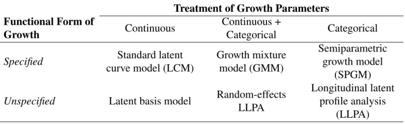
1 Summary of models under consideration
...
442 Percent CES-D scores present at each time point
...
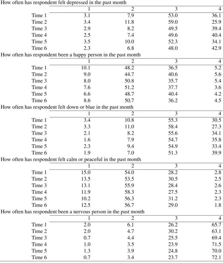
453 Frequency of each response at all time points, in percentage points
...
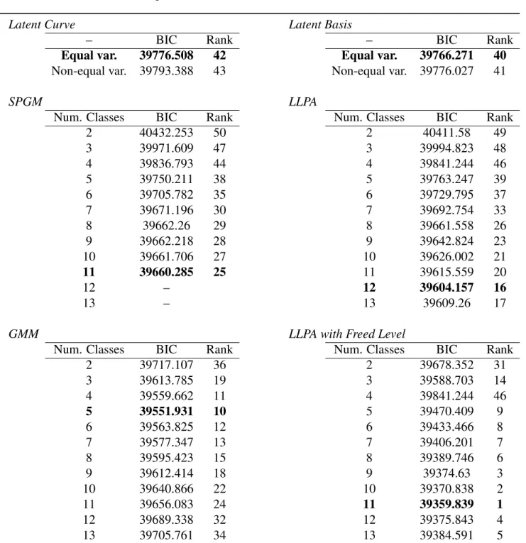
464 Comparative fit of all unconditional models
...
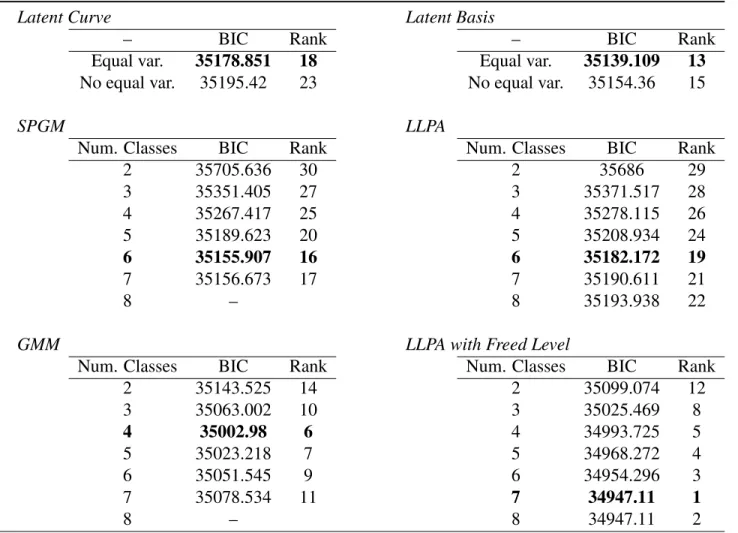
475 Comparative fit for all conditional models
...
486 Covariate effects for the conditional analyses
...
497 Individual RMSRCi values: Unconditional analysis
...
508 Individual RMSRCi values: Conditional analysis
...
519 Individual RMSRMi values: Conditional analysis
...
52LIST OF FIGURES
1 Whole-sample predicted trajectories under all unconditional models
...
542 Whole-sample predicted trajectories under all conditional models
...
553 Predicted trajectories for subjects at the 50th percentile of RMSR
...
564 Predicted trajectories for subjects at the 75th percentile of RMSR
...
575 Predicted trajectories for subjects at the 25th percentile of RMSR
...
586 Predicted trajectories given gender and college attendance
...
591 INTRODUCTION
Researchers are often interested in how behaviors or constructs change and develop over time. As such, recent years have seen substantial development of methods to test longitudinally oriented research questions, such as the multilevel model (MLM; Rauden-bush and Bryk, 2002; Snijders and Bosker, 2011) and latent curve model (LCM; Bollen and Curran, 2006). These methods allow for random variation in the factors that influence change in different individuals – meaning that each subject is characterized by a (poten-tially) unique set of parameters governing the initial level of the phenomenon under study (i.e., a random intercept) and change in this phenomenon to time (i.e., a random slope).
Despite the flexibility of the LCM framework, most extensions of these models make two assumptions about the nature of heterogeneity in the data: (1) that inter-individual differences in growth parameters are normally distributed around a population mean; and (2) that intra-individual change follow a prescribed functional form, usually linear or some lower-order polynomial. Thus, these methods are helpful in describing processes in which the same functional form is thought to describe the shape of change for all individuals, per the first assumption, and the basic shape of this functional form is known, per the second assumption.
The main goal of this thesis is to introduce a modeling framework, longitudinal latent profile analysis (LLPA), which allows for the modeling of trajectories without being subject to either of the above assumptions governing the nature of inter-individual differences or the shape of intra-individual change. To contextualize these developments, I first review the rationale for methods that relax the first assumption – specifically, mixture models, which allow categorically different trajectories for different members of the sample. I then introduce LLPA as a minimally parameterized mixture model, and show how it may be used to make inferences about the nature of change at the whole-sample level. Then I extend LLPA’s potential utility to individual-level analyses, and thus attempt to show how LLPA may make a novel contribution to person-centered research. Finally, I will compare LLPA to modeling methods which also allow fewer assumptions about the nature of intra-and inter-individual difference in the data.
1.1 Longitudinal mixture models in person-centered analysis
illnesses, may alter the rate of change in white matter volume (Bartzokis et al., 2003) the fundamental shape of the growth curve across the lifespan is probably quadratic for each individual.
In psychology, however, researchers are frequently interested in phenomena that may follow trajectories of completely different shapes for different individuals in the sample. A broad class of models that can be implemented for evaluating this heterogeneity is mix-ture models (McLachlan and Peel, 2000). Though a formal treatment of mixmix-ture models will be given later, the basic premise of these models is that they treat subjects as though they come from distinct subpopulations (known as classes or components), allowing for statistical inference to be made on the basis of these subpopulations. Originally conceived as a method of classifying natural phenomena (Pearson, 1894), mixtures have gained use in the social sciences, with both cross-sectional (e.g., Lazarsfeld and Henry, 1968) and longitudinal (e.g., Muth´en and Shedden, 1999; Nagin, 1999) applications.
Titterington, Smith, and Makov (1985) distinguish between direct and indirect appli-cations of mixture modeling. The vast majority of published appliappli-cations of longitudinal mixture models are direct applications, in which the goal is to ascertain subgroup mem-bership – in these models, categorical variation is a substantive outcome of interest. Direct apppications are consistent with the search for meaningful typologies of psychological phe-nomena, a goal which has characterized much psychological work throughout the past cen-tury (e.g., Meehl, 1992). In indirect applications, by contrast, parameters from the mixture model are usually used to ascertain information about the population as a whole, aggregat-ing across clusters; thus, in indirect applications, the categorical latent variable is typically not an outcome of intrinsic interest.
seeks to isolate individuals, or clusters thereof, who show particular patterns of response to any number of variables, including both time-varying indicators (e.g., substance abuse at time t) and covariates. The draw of such an approach is that it allows individuals to be characterized holistically in terms of interactions between any number of internal and external factors working in concert (Bauer and Shanahan, 2007). Proponents argue that this approach is far closer to the reality of complicated developmental processes than variable-centered techniques, which are often applications of regression models emphasizing single factors’ effects controlling for all others.
One substantive area in which person-centered analyses have frequently taken the form of direct applications of mixture models is the developmental etiology of substance abuse. For instance, Schulenberg et al. (1996a) find six trajectories of binge drinking between ages 18 and 24, and link these trajectories post-hoc to a number of covariates (1996b). Their work shows a number of individuals maintaining habits of either minimal, moder-ate, or heavy binge drinking, some decreasing linearly in the frequency of binge drinking, and others (termed ”fling” binge drinkers by the authors) showing a period of increased binge drinking toward the middle of the study period, after which drinking decreases sub-stantially, thus resembling a quadratic trend (Maggs and Schulenberg, 2005). Casswell, Pledger and Pratrap (1996) report a similar quadratic pattern in one subset of their sample, only these individuals experienced peak binge drinking around age 26. Similar findings of heterogeneity have also been reported when considering younger samples (e.g.,King et al., 2000; Chassin, Pitts, and Prost, 2002; Sher, Jackson, and Steinley, 2011), as well as sub-stances besides alcohol such as marijuana (e.g, Schulenberg et al., 2005; White, Labouvie, and Papadaratsakis, 2005; Windle and Wiesner, 2004), and cigarettes (e.g., White, Padina, and Chen, 2002).
that each group is defined by a parametric form. It is possible, however, that assuming linear or quadratic increases in substance use might be an oversimplification of what is occurring in the data. For instance, the ”fling” group of binge drinkers identified by Schulenberg et al. (1996a; 1996b) may not uniformly show a single period of increased binge drinking around college age, as would be implied by the quadratic trajectory found by the researchers. Per-haps some subjects show this trend of one isolated period of heavy drinking during college but, additionally, there are individuals in the sample who show multiple recurring periods of increased drinking, as well as some who show a single period of binge drinking past college age, et cetera. Furthermore, it may be the case that these sub-classifications of ”fling” drinkers are differentiated from one another by covariates (e.g., Wechsler et al., 1995; Weitzman, Nelson, Wechsler, 2003). Therefore, imposing functional forms on tra-jectories of binge drinking across time might sacrifice valuable information required for a truly person-centered approach, both by oversimplifying the true shape of change as it occurs on an individual level, and by obscuring the relationship between these changes and contextual factors.
will now introduce a new mixture model, longitudinal latent profile analysis (LLPA), and discuss several potential indirect applications of this model.
1.2 Longitudinal Latent Profile Analysis
Latent profile analysis (LPA; Gibson, 1959) is a type of mixture modeling that was developed for and has traditionally been applied to data obtained at a single time point on multiple, distinct continuous indicators. Direct applications of LPA are common, and LPA has shown its utility in studies seeking to classify patients into subgroups of symptom profiles, with degree of endorsement of each symptom being an indicator (e.g., Mitchell et al., 2007; Holliday et al., 2009). LPA has also been used in community samples with the aim of determining the level and nature of certain psychiatric issues in the population (e.g., Wade, Crosby and Martin, 2006).
In a basic LPA, the observed score for individuali(i=1,...,N) on indicatorjgiven mem-bership in classkis given by:
y(ijk) =ξj(k)+Eij (1)
whereξj(k) is the true score on indicatorj for classk. Here error is represented byEij ∼ N(0, σ2
j), where σj2 is the residual, or within-class, variance of indicator j across
indi-viduals. Importantly, residuals are assumed uncorrelated with one another across vari-ables within class. Thus class membership, and therefore between-class differences in true scores, is the only source of covariance between the variables; this is termed theconditional independenceassumption.
The traditional LPA framework, which forms profiles based on multiple variables at one time, may be adapted to a longitudinal setting, such that profiles capture differences in a single variable over time. Equation 1 may be reconsidered so thatjindexes occasions of measurement of a single variable, and thus ξj represents scores on this variable across
a class-specific grand mean of the indicators,µ(k), which represents the overall level of the
indicator in class k across time; and time-specific deviations from the overall level, δt(k), which sum to zero and represent the shape of variation around the within-person mean. The longitudinal latent profile analysis (LLPA) may thus be written as:
yit(k) =µ(k)+δ(tk)+Eit (2)
Hereyitrefers not to individuali’s score on itemj, as in Equation 1, but to individuali’s
score at timet(t=1,...,T), given membership in class k. The individual error component is given byEit ∼N(0, σt2), whereσt2is the variance at timetacross individuals. Importantly,
there are no constraints on the values of δt(k) aside from the fact that all values for each class must sum to zero – they simply represent vertical deviations from the overall level at timet. Therefore, the model allows for maximum flexibility, as no parametric relationship between time and the indicator is modeled.
While yit(k) represents the observed score for individual i given membership to class k, one may aggregate over the classes using πk, the proportion of the sample in classk,
to obtain the marginal means and covariance structure for the whole sample. The model-implied marginal means are:
µy =
K X
k=1
π(k)(µ(k)+δ(k)) (3)
whereµy represents a vector of length T containing the estimated marginal means of the repeated measures at each time point; µ(k) is a vector of length T containing the level of
class k, repeated t times; and δ(tk) is a vector of length T containing time-varying shape parameters for classk.
refer to the vector of class-specific means of indicators formed by addingµ(k) andδ(k)
as
ξ(k) for the purpose of brevity; because ξ(k) = µ(k)+δ(k), ξ(k) represents the vector of means at each of time tfor classk. Thus covariance matrix of indicators in the sample is calculated as:
Σyy = K X
k=1
π(k)(ξ(k)−µy)(ξ(k)−µy)0+
K X
k=1
π(k)Σ(k) (4)
The first term refers to the between-class contribution to the marginal covariance ma-trix; the second term refers to within-class contribution to the marginal covariance. The first term models the variances of indicators, as well as covariances between them, as a result of differences in within-class means; in the LLPA, each class’ vector of means repre-sents the unique longitudinal profile of that class. HereΣ(k)is a diagonal matrix, with the within-class variance of repeated measures in classkon the diagonal, and thus the second term of this equation contributes only to the variances of repeated measures, not covari-ances, in the marginal covariance matrix. Thus, all covariance in the observed scores yit
is thought to be explained by the first term, or differences in between-class means. Thus, conditional independenceassumption, which holds that covariances between indicators are accounted for by class membership, holds as in Equation 1.
offenders by using subscales of the Brief Symptom Inventory (BSI) as indicators, and in-formation about offense history (e.g., violent vs. nonviolent offending, age at first offense) as covariates. However, the person-level predictors considered in this thesis are thought to be antecedent to the groupings themselves and are thus fundamentally different in meaning from the repeatedly measured class indicator (Lubke and Muth´en, 2007; Marsh, Ludtke, Trautwein, and Morin, 2009). For this reason, only time-invariant covariates are considered formally here. Considering only time-invariant predictors in the current analysis helps to make the distinction between covariates and indicators somewhat less hazy: indicators are a time-varying dimension, while covariates are time-invariant antecedents influencing class membership but not the shape of the trajectory in each class.
The class probabilities, dependent on covariates, are defined through a multinomial logistic regression:
π(k)(zi) =
exp(θ0(k)+θ(k)0zi)
PK
k=1exp(θ (k)
0 +θ
(k)0
zi)
(5)
whereθ(0k) is a class-specific multinomial intercept for classk, andθ(k) is the multinomial regression coefficient relating the covariate vectorzito membership in classk. As in most
applications of multinomial logistic regression, one class is treated as a reference class, in whichθ0(k)andθ(k)are constrained to zero for model identification.
The vector of model-implied means for the repeated measures given zi can thus be
given by a slightly altered version of Equation 3, which conditions on the covariate vector
zi:
µyi =
K X
k=1
π(k)(zi)(µ(k)+δ(k)) (6)
Given Equations 5 and 6, expected trajectories can be calculated and plotted at different values of the covariates, as is often done in multilevel modeling and latent curve analysis (Preacher, Curran, and Bauer, 2006). This strategy can serve a number of purposes. First, one can generate values of π(k)(z
medium, and high) holding other covariates constant (e.g., at their means) using Equation 5, and then use the resultant value to generate a predicted trajectory using Equation 6. Such results may be useful for determining the nature of the relationship between predictors and trajectories on average in the population. However, LLPA can be extended further to provide insight into the shape of change at the individual level; I now explore the two main ways, using Equations 5 and 6 and extensions thereof, of using LLPA to make individual predictions.
1.3 Individual-level inference in LLPA
Pursuant to the goals of person-centered analysis, it is often of interest to plot model-predicted trajectories for individuals in the sample. Assessment of model fit at the indi-vidual level is common in the MLM literature (Rabe-Hesketh and Skrondal, 2008), but relatively rare in mixture models. However, these individual model-implied trajectories can provide information about how well the model approximates the observed trajectories at the individual level.
LLPA can be used to accomplish this goal in two ways. First, one can generate pre-dicted values ofπ(k)(zi)for each individual in the sample, given each individual’s vector
of predictors zi – in other words, rather than using Equations 5 and 6 to calculate
hypo-thetical trajectories given values of covariates chosen by the researcher, one could input the combination of covariates specific to individual ito obtain that individual’s predicted trajectory.
In this formulation,π(k)(z
i)is considered to be the predicted probability of class
mem-bership, and is thus used to weight each class’ trajectory. However, π(k)(z
i)is essentially
vector of length T consisting of all of subject i’s observed scores, referred to as yi, this posterior probability is given by:
τi(k)(zi) =
π(k)(z
i)f(k)(yi|zi) f(yi|zi)
(7)
wheref(k)(y
i|zi)is the class-specific multivariate normal density foryiconditional onzi;
andf(yi|zi)is the marginal multivariate normal density foryi conditional onzi.
Thus, the posterior probability of personibelonging to classkis calculated by weight-ing the class-specific likelihood by the whole-sample membership proportion for class k given covariatesz, and dividing by the whole sample likelihood. Importantly, each mem-ber of the sample has a nonzero probability of belonging to each class, and all posterior probabilities over theK classes sum to 1 for individuali.
Just as the whole-sample trajectories can be calculated by weighting class-specific jectories according to class membership proportion (found in Equation 6), individual tra-jectories can be calculated weighting by an individual’s posterior probability of belonging to a particular class. Thus, an individual’s model-predicted trajectory is given by:
ˆ yi =
K X
k=1
τi(k)(zi)(µ(k)+δ(k)) (8)
on fixed effects. By contrast, Equation 8 represents a conditional predicted trajectory, as it incorporates the equivalent of a random effect inτi(k)(zi)in weighting the class’
trajecto-ries; thus trajectories predicted using Equation 8 with sample values in place of population parameters are empirical Bayes estimates.
Both the marginal and conditional predicted trajectories for individuals in the sample may be of interest, and they may serve distinct but complementary purposes. In particular, gauging the discrepancy between an individual’s observed and marginal predicted trajecto-ries may yield an impression of whether a given individual is ”typical” given a certain set of covariates or predisposing factors (e.g., Skrondal and Rabe-Hesketh, 2003). By contrast, the discrepancy between an individual’s observed and conditional predicted trajectories will be used to index individual-level model fit (Coffman and Milsap, 2006; Skrondal and Rabe-Hesketh, 2009).
1.4 Random-effects LLPA
It is often of greater interest in longitudinal research to ascertain differences in the shape of a phenomenon, rather than differences in level. However, in the LLPA as it is currently formulated, differences in overall level may have more influence on class membership than shape, even if heterogeneity in shape is the primary outcome of interest. For example, given the vast heterogeneity in overall level of depression among adolescents (e.g., Dekker et al., 2007), one might imagine that classes based on longitudinal measures of depression would largely reflect variance in level, potentially obscuring interesting heterogeneity in shape.
One potential modification to the LLPA that may address this concern is to allow for within-class variability in the level parameter. In this scenario Equation 2 would be altered as follows:
yit(k)= [µ(k)+αi(k)] +δ(tk)+Eit (9)
of Equation 9 in brackets refers to a person-specific level parameter, comprised of mean
µ(k) and person-specific deviation α(ik), where these deviations are normally distributed across persons within-class.
In this model, referred to here as the random-effects LLPA, fewer classes would likely be needed to approximate heterogeneity in profiles of growth, and the latent class variable would capture more information about the shape of change for the variable, which may produce more substantively interesting and interpretable profiles. Importantly, this also means that covariates, in that they are linked to the variables exclusively through class membership, may now only explain one of two pools of variability in the level parameter. The random-effects LLPA will be further explored in an empirical analysis later in this thesis.
Both with and without within-class random effects for level, LLPA’s lack of assump-tions about the functional form of growth may help to preserve a greater level of detail about within-person variability than standard extensions of the LCM. However, LLPA is not the only model that has been proposed to facilitate person-centered analysis through flexible modeling of change. In order to better understand the unique features of LLPA, I will now consider its potential advantages and disadvantages relative to two existing techniques allowing different types of within- and between-person variability: longitudinal mixture models, and single-class extensions of the latent growth model allowing different forms of growth.
1.5 Relation to other models
One sort of longitudinal mixture model that has gained popularity in recent years is the semiparametric growth model (SPGM; Nagin and Land, 1993; Nagin, 1999). In an SPGM, subjects are assumed to come fromK classes, with each classkdefined by its own growth equation. For instance, a linear SPGM would be of the form:
whereβ0(k)andβ1(k) vary between (not within) classes, andEij ∼N(0, σ2t).
If time is centered at the midpoint, the intercept term β0(k) Equation 10 represents the within-class average level of the observations, just like the level parameter µ(k) in Equa-tion 2. Where SPGM differs from LLPA is in the specificaEqua-tion of a parametric relaEqua-tionship between the repeated measure and time: whereas the shape parameterδt(k) in Equation 2 does not directly incorporate any parametric function of time, the termβ1(k)timeitin
Equa-tion 10 imposes straight-line growth. While EquaEqua-tion 10 represents linear growth in each class, quadratic or cubic growth can also be modeled (e.g., Karp, O’Loughlin, Paradis, Hanley, and Difranza, 2005; Tucker, Orlando, and Ellickson, 2003), as can more complex functions such as Gompertz and logistic curves (Grimm and Ram, 2009; Grimm, Ram, and Estabrook, 2010). The disadvantage of this approach, relative to LLPA, is that the researcher must know the function a priori, whereas this function may often be unknown or uncertain. An advantage of SPGM over LLPA, however, is that the specification of a parametric form allows for individually-varying times of observation.
Just as the LLPA can be extended to incorporate within-class variance of level, so too can the SPGM be extended to allow within-class variance of growth parameters. Longi-tudinal mixture models that allow growth parameters to vary within-class are generally referred to as growth mixture models (GMM; Muth´en and Shedden, 1999). A GMM of linear growth would be given by:
yit(k)=β0(k)+β1(k)timeit+Eit (11)
where
β0(k)
β1(k)
∼N
µ(βk)
0
µ(βk)
1 ,
σβ2(k)
0
σβ(k)
0β1 σ
2(k)
β1 .
assumed to vary normally within class around the class mean; thus β0(k) and β1(k) are es-sentially random effects within class. Furthermore, one can formulate longitudinal mixture models in which different components have different functional forms of growth, such as one class showing linear growth and another class with quadratic growth (Muth´en and Muth´en, 2000; Muth´en, 2001). Freeing the variance of growth parameters changes their interpretation, a point that has been debated widely within the context of direct applications of mixture models (Nagin, 2005; Nagin and Tremblay, 2005; Muth´en, 2006). Rather than being a parameter defining the entirety of the group, in a GMM the parameter value simply represents a mean around which there is random variance, just as in a single-class latent growth model. Importantly, however, these interpretational changes are most relevant in direct applications, given that within-class parameters are typically not interpreted in indi-rect applications. In this sense, what both GMM and the random-effects LLPA represent is a combination of categorical and continuous treatments of variance in growth param-eters, since these growth parameters are allowed to vary categorically according to class membership but also continuously around a class mean parameter value.
The LLPA and other longitudinal mixture models (SPGM, GMM) are similar in that they treat trajectories as varying categorically between subjects and thus relax the standard LCM’s assumptions about the nature of inter-individual differences. Unlike the SPGM and GMM, however, the LLPA is also minimally parameterized with respect to the shape of change, and thus relaxes assumptions about the nature of intra-individual differences. Another model that shares LLPA’s lack of a pre-specified functional form is a LCM with completely freed loadings, sometimes referred to as the latent basis LCM (Meredith and Tisak, 1984, 1990; McArdle and Epstein, 1987). This model is specified as:
Yit =β0i+β1iλt+Eit (12)
from the data. Just as an LLPA is essentially an SPGM without pre-defined functions of time, a latent basis model is an LCM without pre-specified loadings for time, and therefore no pre-defined functional form. Two loadings are fixed at 0 and 1 to set the metric of the factor; the remaining loadings are estimated freely. This is contrasted with models such as a linear LCM, in which the loadings ofλtare fixed at linearly increasing values, usually [0,
1, 2,...,T-1]; unlike these models, time is unstructured in the latent basis model. Because the loadings of time are freely estimated, the metric of time is not always easily interpreted; McArdle (2004) recommends setting the first and last loadings at 0 and 1 respectively, in which case the loading of each time point represents the proportion of total change that has occurred at timet. This particular parameterization is most useful if change is monotonic.
Though both the loadings and the growth factors lose some degree of interpretability under this approach, the latent basis allows not only for a nonlinear functional form but for the lack of any a priori specification of functional form at all. As with LLPA, this degree of flexibility can be greatly beneficial in modeling change when the functional form of intra-individual change is unknown. For instance, Grimm (2007), modeling the relationship between depression and academic achievement between ages 7 and 14, finds that a latent basis model provides an excellent fit to the data; similarly, Grimm and Ram (2009) find that a latent basis model very well approximates the fluctuations in cortisol over trials of a stress test. However, a disadvantage of the latent basis model is that it assumes that the same basic shape of change is the same for all individuals, with only differences in magnitude or direction.
1.6 Summary and Research Aims
2 METHODS
2.1 The National Longitudinal Survey of Youth
Data come from the 1997 National Longitudinal Survey of Youth (NLSY97), an on-going longitudinal study that has collected data on education, employment, government program participation, crime, family life, substance abuse, and health in a nationally rep-resentative sample of adolescents. From 1997 to 2000, data were collected at one-year intervals; thereafter, data were collected at two-year intervals. Information sources in-cluded face-to-face and computerized interviews with subjects and their parents, as well as examination of school and administrative records. For the current study, I examine data taken from six of the time points: 2000, 2002, 2004, 2006, 2008, and 2010.
From the larger NLSY dataset a smaller sample (N = 1686), consisting exclusively of individuals who were 14 years old at the time of their first interview in 1997, is analyzed. The age requirement ensured that all subjects were transitioning from adolescence to adult-hood between 2000 and 2010. The sample was 50.4 percent male, and relatively ethnically diverse, with 26.8, 20.0, .08, and 50.5 percent of respondents identifying as Black, His-panic/Latino, mixed race, and neither Black nor HisHis-panic/Latino, respectively. For ease of model fitting, this sample includes individuals who were interviewed at least half of the time points. Patterns of missing data are shown in Table 2.
2.2 Measures
representing all of the time and 4 representing none of the time. The data were coded such that higher values were indicative of less depression. An aggregate score was created from these five items, which showed moderately good internal consistency, with Cronbach’s alpha of .76, .76, .77, .77, .80, and .81 at each of the successive six time points, respectively. Four covariates were also included in the conditional analyses. First, given the frequent finding that women tend to report higher levels of depression than men, gender was in-cluded as a covariate in the model, coded as 1 if the subject was female and 0 otherwise. Race was also included in the model, coded as 1 if the subject was Caucasian and 0 other-wise. In order to consider theories relating physical and mental health in development (e.g., Repetti, Taylor, and Seeman, 2002) we considered parent ratings of the subject’s general health at age 13, two years before the subject’s first interview. Parent-rated health was an ordinal variable, coded from 1-5, with lower scores representing better overall health. Fi-nally, given that there are some reports of different clinical patterns among college students and their non-college-attending counterparts (e.g., Gfoerer, Greenblatt, and Wright, 1997; Blanco et al., 2008), class membership was also regressed on a binary variable representing college attendance, coded as 1 if the subject attended college by age 23 and 0 otherwise.
2.3 Analysis
2.3.1 Model Fitting
last ones freely estimated; (5) a longitudinal latent profile analysis (LLPA) with fixed level and shape factors; and (6) a longitudinal latent profile analysis with a random effect for level within class (LLPA-RE).
2.3.2 Model Comparison at the Global Level
For the mixture models, the Bayesian Information Criterion (BIC; Schwartz, 1978) was used to select the optimal number of classes. The BIC is equal to−2×log(LL)+q(log(N)), whereLLrepresents the log-likelihood of the model, qrepresents the number of repeated measures, andN represents the sample size; a lower BIC thus indicates a stronger fit and more model parsimony at the global level. Both across models and within solutions for the same model (e.g., a 4-class LLPA vs. a 5-class LLPA), BIC was used to compare fit. 2.3.3 Individual Level Analysis
Assessment of fit at the individual level proceeded via the Root Mean Square Residual (RMSR), as defined by Coffman and Millsap (2006). The RMSR directly measures the proximity between individuali’s observed trajectoryyi, and individuali’s model-predicted trajectory. The model-predicted trajectory is defined two ways: first as the marginal pre-dicted trajectory given by Equation 6, µyi, and second as the conditional predicted tra-jectory given by Equation 8, yˆi. Thus, the individual fit to the marginal and conditional predicted trajectories will be assessed, and termed RM SRM i andRM SRCi respectively
and defined as:
RM SRM i =
s PTi
t=1(yit−µyit)2
Ti
(13)
RM SRCi =
s PTi
t=1(yit−yˆit)2
Ti
(14)
whereTiis equal to the number of times at which each individualiis assessed.
not take into account any measure of model parsimony; thus, it is exclusively a measure of closeness of fit and not necessarily generalizability.
For the conditional analyses, the RMSR was calculated two ways – first using Equation 14, yieldingRM SRCi, the RMSR comparing subjecti’s observed and posterior-predicted
trajectories, and then using Equation 13, yieldingRM SRM i, the RMSR comparing subject
i’s observed and prior predicted trajectories given values of covariates. The RMSR was
ex-amined only using equation 14 in the unconditional analysis. The reason for this seeming discrepancy is that, in an unconditional analysis, there are no covariates on which to condi-tion the prior probability of class membership and thus the prior-predicted trajectories are not meaningful at the individual level. First, RMSR values were compared among all of the models, to see if any models provide closer fit to individual data than others.
Then, in order to determine the possibility that models fit differentialy well for indi-viduals with different values of covariates, I examined Pearson’s correlation coefficients relating RMSR values (RM SRCi in both the conditional and unconditional analyses, and RM SRM i in the conditional analysis) to the four covariates included in the conditional
3 RESULTS
3.1 Overall model fit
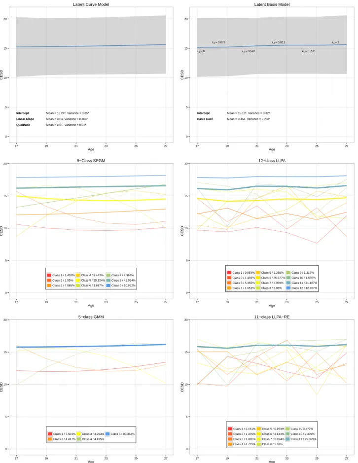
Table 4shows the BIC values for all unconditional models that were tested, ranked according to overall standing (with lower BIC values indicating better performance and thus being ranked higher). The latent curve and latent basis models performed poorly relative to other models; among these options, however, BIC was lower in the versions of both models in which the residual variances of all time points were assumed equal. The mixture models with only categorical variation between latent classes in growth parameters showed wide variation in the degree of fit. Solutions with more classes fit better, with an 11-class solution fitting best in the SPGM – however solutions with more than 11 classes did not converge, and the best likelihood was replicated in neither the 10- nor the 11-class solution. Thus, a 9-class SPGM is considered in further analyses, as this was the last solution at a probable global maximum. Fit was better in the LLPA than in the SPGM; a 12-class solution was the best fit. The GMM and LLPA-RE, which allow both categorical and continuous variation in growth parameters, fit the data the best overall. In the GMM a 5-class solution fit the data the best. In the LLPA-RE an 11-class solution represented the best balance of fit and parsimony. Importantly, this was the best fitting model in the whole sample, with a BIC value almost 200 points below the best-fitting GMM.
latent curve and latent basis models). Second, regardless of the specification of between-person variation in growth parameters, models which do not require pre-specification of functional form (the latent basis model, LLPA, and LLPA-RE) fit better than models that do (latent curve model, SPGM, and GMM).
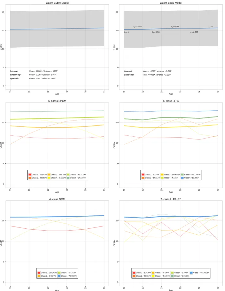
Findings related to the conditional analysis, which are shown in Table 5 showed a few differences from the unconditional analysis. First, models with fewer classes were gen-erally favored by the BIC in the mixture model solutions, likely reflecting the fact that models with the added complexity of covariates cannot accommodate more parameters re-lating to class membership. Second, findings related to the specification of inter-individual difference in trajectories were somewhat more equivocal than in the unconditional model. Unlike in the unconditional analysis, the BIC did not favor models with exclusively cate-gorical differences between individuals in growth parameters (the LLPA and SPGM) over those with continuous inter-individual variation in growth parameters (the latent curve and latent basis models). In fact, the latent basis model fit the data better than any of models al-lowing exclusively categorical differences in growth parameters, including the best-fitting LLPA. However, as in the unconditional analysis, models allowing both continuous and categorical variation between individual growth parameters showed the best balance of fit and parsimony. As before, the best-fitting model in the data was a LLPA with random effects; this time a seven-class solution was favored by the BIC. Thus, the major trends of the unconditional analyses were basically replicated when covariates were added: mod-els allowing both continuous and categorical variation in growth parameters (GMM and LLPA-RE) showed the best fit to the data, as did models in which the functional form of growth was not pre-specified (latent basis model, LLPA, and LLPA-RE).
3.2 Whole-sample predicted trajectories
transparency of each line is used to indicate the proportion of individuals in the corre-sponding class. In both models the latent curve and latent basis models, only the mean of the intercept coefficient was significant, indicating that only initial level of depression was significantly different from zero. However, the variance of all of the growth coefficients – intercept, linear slope, and quadratic slope in the latent curve model; intercept and basis co-efficient in the latent basis model – were significant. These combined findings – no growth coefficient having a significant mean, but each having a significant variance – suggest that while at the aggregate level there is no overall change in depression over time, individuals differ in the extent to which their self-rated depression changes over time.
One trend that characterized all of the mixture models is that they all placed the majority of the sample in classes defined by high CES-D scores that do not change much over time. Where the models differ is in their representation of the rest of the sample. In the SPGM, classes were differentiated from one another most by overall level; only three classes – classes 2, 4, and 6, comprising a total of 5.6% of the sample – were characterized by a significant quadratic trend, and only class 7, comprising roughly 8.0% of the sample, showed a linear increase in CES-D score over time. In the GMM, three classes – classes 2, 3, and 4 – were defined by any change over time; the remainder of the sample fell into classes 1 or 5, which where characterized by either low or high overall CES-D scores, neither of which increased or decreased over time. Thus, though there were fewer classes in the GMM than in the SPGM, roughly the same proportion of the sample, 12.1%, fell into classes characterized by any sort of change in depression over time.
of change that, by graphical examination, appear to represent a variety of potential func-tional forms; classes’ trajectories range from those with small periodic fluctuations, such as classes 2 and 3, to those with large increases or decreases at one age, such as classes 1, 5, and 10. The LLPA-RE is similar in that roughly 25%of the sample fell into classes characterized by change over time, and these changes were not well-defined by any single functional form, but there were two main differences. First, here only one class, class 11, was needed to characterize individuals with high CES-D scores that did not change over time, as opposed to three. Second, the remaining classes are distinguished from one an-other less by differences in overall level of CES-D, and more by differences in shape, as represented graphically by the fact that trajectories overlap a great deal in overall level of CES-D scores but show wider differences in their profiles of change over time.
Results in the conditional model are presented in Figure 2. As before, neither the latent curve nor the latent basis models were characterized by a great deal of change over time. While fewer classes were found in almost all mixture models, the shapes of the trajectories defining each class were similar, and two main trends in the unconditional analysis were replicated. First, most of the sample fell into trajectories with high CES-D scores that did not change over time, with more sparsely-populated classes representing individuals with lower scores who did change over time. Second, in models in which some within-class variation in overall level of CES-D score was allowed (the GMM and the LLPA-RE), classes were less differentiated from one another by level and more by the overall shape of each trajectory.
3.3 Effects of covariates
similar, with a highly significant effect of gender on the intercept (z= 7.054,p<.001) and no other effect on either the intercept or latent basis coefficient approaching significance.
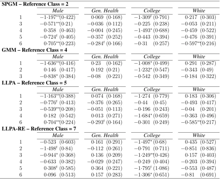
Table 6 shows the results of logistic regressions using all of the covariates as predictors of class membership for each mixture model. In all models, the modal class – which in each solution was characterized by high CES-D scores and minimal change over time – is used as the reference class.
In the SPGM, members of classes 1 and 3, which showed low overall CES-D score, were more likely to be female, whereas members of class 6, which showed high overall CES-D scores, were less likely to be female. Members of class 6, the only class with higher overall CES-D score than the reference class, were also less likely to be white. Members of class 4, which was characterized by lower scores (corresponding to increased depression) at later ages, were less likely to have completed college.
In the GMM, the only covariates with any significant partial effects were gender and college. Members of classes 1 and 3, which were characterized by either lower overall CES-D score (class 1) or low CES-D score which increased over time (class 3), were more likely than members of the reference class (class 4) to be female. Members of class 1 and class 2, which was characterized by decreasing CES-D score, were also less likely to attend college than members of the reference class.
Interestingly, members of class 4, which was defined by the decreasing CES-D scores cor-responding to an increase in depression at later ages, were less likely to have attended college by age 23, but this effect was not significant for any other classes.
In the LLPA-RE, only class 3 was distinguished from the reference class by gender; thus, only members of the class with lowest and most widely-varying CES-D scores were more likely to be female. Members of this class were also less likely to have attended college by age 23, as well as members of class 1, which was also characterized by low and widely-fluctuating CES-D score, and class 6, in which CES-D score started out high but dropped precipitously at the later ages.
3.4 Individual fit
Root mean squared residual (RMSR) scores were calculated for each individual under each model using posterior-predicted individual trajectories (given Equation 14) for both the conditional and unconditional analysis; RM SRM i values for each individual under
each model were calculated using Equation 13 for the conditional analysis only. Their rela-tionship to a number of covariates, including the four that were examined in the conditional model – gender, race, college attendance, and parent-rated general health – as well as the number of missing CES-D scores, were then examined. The intent with this analysis was not hypothesis-driven, but instead focused on whether, both in the unconditional analysis in which none of these covariates was included and in the conditional analysis in which the covariates were included, any given model fit individuals with certain values of the covariates better or worse.
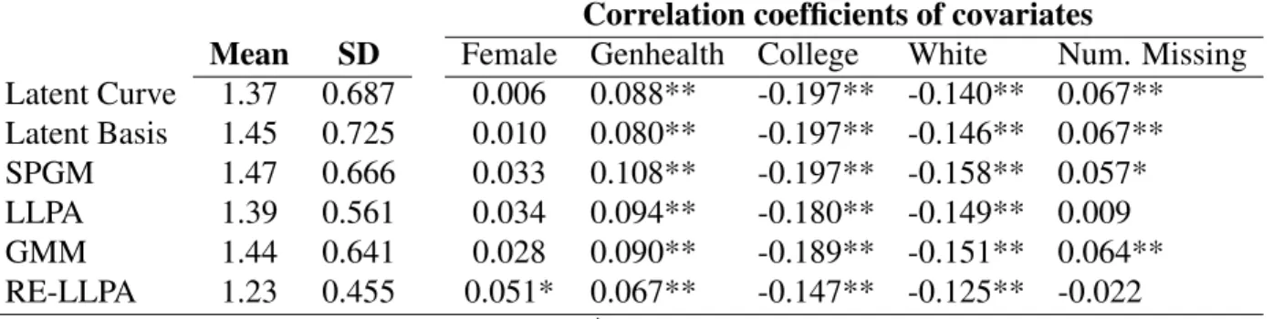
The means ofRM SRCi scores for the unconditional analysis are presented in Table 7.
The averageRM SRCiscores were relatively similar in most models but were considerably
lower in the LLPA-RE than in the other models, indicating that trajectories fit more closely to individual data in the LLPA-RE than in other models. RM SRCiscores were strongly
in white subjects, subjects with better overall general health, and subjects who attended college. Interestingly, gender was not significantly related to individual fit in any model except for the LLPA-RE, in which being female was associated with worse overall fit. An-other interesting finding is that the number of missing time points was significantly related to individual fit in all models except for the LLPA and the LLPA-RE models, potentially suggesting closer fit of these models to subjects with higher degrees of missing data.
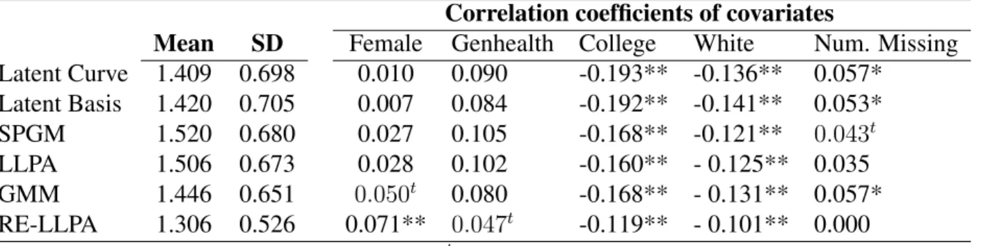
The means ofRM SRCi scores for the conditional analysis are shown in Table 8. As in
the unconditional analysis, the LLPA-RE fits the data more closely at the individual level than any other model; however, the difference in fit was smaller than in the unconditional analysis. As before, race and college attendance were strongly related to individual fit and gender was not; however, in the conditional analysis, there was no relationship between general health and any of the models’ RM SRCi values except for the LLPA-RE at the
trend level. The previous pattern of relationships betweenRM SRCiand missingness were
replicated: there was no significant relationship between missingness and individual model fit in the LLPA and the LLPA-RE, but significant (or, in the case of the SPGM, marginally significant) relationships to missingness in all other models.
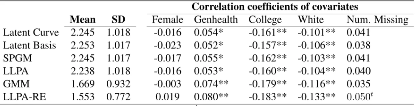
Finally, the means ofRM SRM ivalues in the conditional analysis are shown in Table
9. Values overall were higher than theRM SRCi values in either the conditional or
uncon-ditional analyses; however, the values for both of the models allowing both continuous and categorical variation in growth paramters (GMM and LLPA-RE) were the lowest, indicat-ing closest overall fit at the individual level in these models. As with theRM SRCi, there
was no overall relationship between gender andRM SRM i values. There was, however, a
significant relationship between fit and race, general health, and college attendance in every model. There was no significant relationship between fit and missingness in any model.
closer fit to each individual’s data, on average, than any other method under consideration. Second, the inclusion of covariates in the analysis did not lead to much attenuation of the relationship between covariates and fit, as indexed either using the RM SRCi based
on posterior-predicted individual trajectories or the RM SRM i based on prior-predicted
individual trajectories. Finally, when considering fit to each individual’s posterior-predicted trajectory (i.e.,RM SRCiin either the unconditional and conditional model, the fit of LLPA
and LLPA-RE is not as greatly affected by missingness of CES-D scores than the other models.
3.5 Individual Prediction
For each individual, a prediction plot given the best fitting unconditional model – the 11-class LLPA-RE – was created. These plots are shown for six individuals in the sam-ple, in Figures 3-5. In the first panel of each plot is the 11-class LLPA-RE solution, with the lines weighted (both using line thickness and transparency) by the subject’s posterior probability of belonging to each class. From this plot one can visualize how well each class represents a given individual’s model-implied trajectory. In the second panel is the individual’s observed and model-implied trajectories, as well as 100 predicted trajectories generated by the bootstrap methods of Pek, Bauer, and Losardo (2011) using the covariance matrix of model parameters. By visualizing the uncertainty around the individual predicted trajectory nonparametrically, one can get a sense of the error around each individual obser-vation.
In Figure 3, the plots for subjects 1266 and 1401 are shown; these two individuals had
RM SRCiscores at the median for the sample, and thus they represent the exact midpoint
of individual model fit. In Figure 4, the plots for subjects 286 and 560 are shown; these two individuals hadRM SRCi scores at the 75th percentile and thus represent relatively poor
individual model fit.
Finally, in order to demonstrate the graphical capabilities of LLPA with covariates, predicted trajectories were created by using hypothetical configurations ofzi in Equation
5 to create prior probabilities of class membership. Figure 6 shows one such plot, which compares subjects on the basis of gender and college attendance (holding race constant at white, and general health constant at the sample average). The plot provides insight into one trend that might not have been apparent from examination of the model parameters alone: while female college attendees have higher CES-D scores than non-attendees, indicating generally lower depression for the entire study period, male college attendees and non-attendees seem to diverge in depression only in the later ages.
The current analyses compare the LLPA framework to other analytic approaches in the context of only one dataset. It may be the case that LLPA was favored by fit indices due to idiosyncratic characteristics of the NLSY data. This possibility is explored next using a brief proof-of-concept simulation, which examines the sensitivity of a number of these models to random noise in the data.
3.6 Proof-of-concept simulation
In the preceding analyses, both variations of the LLPA framework – with and without a random effect of level – were favored by the BIC over the latent basis and latent curve models (as well as other models). At the same time, all models tested gave the impression of minimal change over time for most individuals. This conclusion stems from the lack of significant growth coefficients in either the latent curve or latent basis models, as well as as the fact that in the mixture models most individuals were in groups characterized by minimal change. These general findings, in combination, raise the concern that the impression of LLPA models’ superior fit may in fact be driven by overfitting in the absence of systematic change in the data.
with no growth of any sort and tested whether an LLPA would be spuriously favored over an intercept-only latent curve model. In order to do this, I simulated six time points for 1686 cases (as there were 1686 individuals in the original sample). The random intercept was set to have a mean of 15.24 and a variance of 3.35, as these were the mean and variance of the random intercept in the latent curve model fit in the unconditional analysis. Similarly, residual variance at each time point was set at 3.166, as this was the estimated residual variance in this latent curve model. The slope coefficient was fixed at zero and had zero variance.
While generating data from a latent curve model may partially address the concern that an LLPA might pick up random noise in the data and be spuriously chosen over a LCM, the original data is ”noisy” in two ways that simulated data typically is not. First, where the simulated data is fully continuous, the original data was on a 20-point scale and scores could only take on integer values. Second, there was no missingness in the simulated data, whereas there was a moderate degree of missingness in the original data. To rectify these two discrepancies, I altered the simulated dataset such that all values were rounded to the nearest whole number, and values were deleted to simulate the pattern of missingness shown in Table 2.
curve model was nevertheless favored over any of the LLPA models.
4 DISCUSSION
This thesis introduced longitudinal latent profile analysis (LLPA), a mixture model which allows for maximum flexibility in the shape of intra-individual change and inter-individual differences in longitudinal analyses. The LLPA models growth in terms of two parameters – level and shape – and allows these parameters to vary categorically between people. This model was extended to allow for a random effect of level within each class (LLPA-RE), which allows class membership to reflect more shape-based differences across individuals. The LLPA-based methods were applied to a study of depression in a nationally representative sample of adolescents, and the fit of these models was compared with a num-ber of comparable latent curve models and parametric mixture models at the whole-sample level using the Bayesian Information Criterion (BIC). This thesis also examined the use of individual fit statistics, particularly the individual root mean squared residual (RMSR), to examine the different models’ fit at the individual level, and examined graphical methods for individual-level inference.
4.1 Fit at the whole-sample level
The main question regarding these findings is whether the non-parametric shapes un-covered by LLPA and LLPA-RE are valid points from which to draw inference, or simply capturing random noise in the data. A number of the current findings offer a good deal of evidence that the LLPA analyses picked up signal, and not noise, in the data. The BIC was reliably lowest in the LLPA-RE, both in models with and without covariates, and impor-tantly the BIC reflects both parsimony and fit. This finding likely reflects the minimally restrictive nature of the LLPA-RE, which neither forces all individuals to have the same shape of growth, nor the same overall level of depression as everyone in their class. In-terestingly, after the LLPA-RE the second-lowest BIC scores tended to be observed in the GMM, suggesting the possibility that allowing flexibility in the representation of between-person differences in growth parameters may be the best way to optimize fit and parsimony simultaneously.
Further evidence for the LLPA’s lack of susceptibility to conflating random noise with systematic change comes from the proof-of-concept simulation. These results suggest that, in the presence of only level differences, neither the LLA nor its random-level extension will erroneously find nonlinear shapes in the data. The LLPA-RE only found one class, and this class was only characterized by a significant mean and variance for level, with no change in shape. Even an LLPA solution which erroneously divided the sample into classes found these classes to be differentiated only by level, with complete stability of scores across times for all groups. More systematic simulations in future work will further assess LLPA methods’ sensitivity to error variance in the lack of any meaningful change in the data. One important focus of potential future work will be investigating the effect of heteroscedasticity of error – importantly, the simulation assumed that error variance was distributed identically for all classes, but this may not be a tenable assumption in the CES-D.
for LLPA’s findings at the lower end of the CES-D’s range being attributable to random noise as opposed to systematic change: responses at the extreme end of the scale are nec-essarily more error-prone than observations closer to the mean. While the CES-D has been shown to have comparable internal consistency and test-retest reliability in both depressed and non-depressed populations (Radloff, 1997), it is important to consider the possibility that non-parametric shapes among those with higher overall degrees of depression are an artifact of random, unsystematic fluctuation in depression.
It is also important to consider, however, the difference between unsystematic error and meaningful instability across time – i.e., state variance as opposed to trait variance in depression. This distinction has been raised with regard to the CES-D in adolescents by Dumenci and Windle (1996), who applied a latent trait-state (LTS) model. Using the full D, the authors determined that there was a significant component relating CES-D scores to trait-level depression, as well as a significant amoung of state-level variance. They hypothesize that the relatively low test-retest reliability of the CES-D (Lin and Ensel, 1984) may in fact be a byproduct of the fact that the CES-D measures a great deal of state variance in depression, which, though it represents meaningful time-to-time fluctuation, is often conflated with measurement error (Nesselroade, 1988).
not necessitate interpreting each predicted increase or decrease in CES-D score for each class; it may be of interest to simply differentiate individuals who experience change from those who do not. By contrast, parametric mixtures such as SPGM, in hypothesizing a particular form of growth (e.g., linear or quadratic), are much more commonly directly interpreted as being representative of a particular type of growth or decay.
4.2 The effect of covariates
The effect of covariates on growth was relatively consistent across models. All found that female participants generally reported higher overall levels of depressive symptoma-tology, which is consistent with the widely-reported finding that women experience depres-sion with higher frequency than men (e.g. Nolan-Hoeksema, 1990; Kessler et al., 2005). Results related to race and parent-reported general health were generally minimal, with only a few inconsistent findings relating CES-D score to either covariate.
The results present a complicated picture of the relationship between college attendance and CES-D score, with only the mixture models detecting any difference in probability of college attendance between the classes. However, all of the mixture models isolated at least one class with a lower probability of college attendance than the reference class; in the SPGM, GMM, and LLPA, this was a class with decreasing values of CES-D, corre-sponding to increased depressive symptomatology at the later ages. Given that educational attainment and SES are highly correlated, and that low SES is strongly linked to increased depression (Lorant et al., 2003; Everson, Maty, Lynch, and Kaplan, 2002), it may be the case depressive symptomatology worsens at later ages among college non-attendees after the socioeconomic effects of not having attended college (e.g., instability of employment) begin to manifest.
classes, each of which were characterized by low CES-D score at some point in develop-ment. This finding stands somewhat in contrast to the results of the SPGM, GMM, and LLPA, that individuals with increasing levels of depression across early adulthood, but not those with generally high levels of depression or decreasing levels of depression, are less likely to go to college. This discrepancy raises the possibility that more strictly parameter-ized methods (e.g., SPGM, GMM, and LLPA without random effects for level) may find that a covariate is linked to a given shape which no longer holds once a more flexible model is applied.
4.3 Individual-level fit and prediction
A number of the interesting features of LLPA are illuminated when considering the model in terms of inference at the individual level. In particular, the individual RMSR as presented by Coffman and Milsap (2006) offers two different types of conclusions about the relative fit of all models considered. TheRM SRCi, which compares each individual’s
observed trajectory to the one that would be predicted from that individual’s posterior prob-ability of belonging to each class, indicates that in general the LLPA-RE yields predicted trajectories for each individual that are closest to his or her observed data. When covari-ates are included in the model, the LLPA-RE is still the closest fit to the data; however this difference in fit is somewhat attenuated. The second individual fit statistic consid-ered, RM SRM i, represents something different from the RM SRCi: in conditioning on
covariate-based prior probabilities, it indexes how closely the covariates predict the ob-served trajectory for each individual in the sample. Despite the fact that there were rel-atively few differences between any of the models in findings at the aggregate level with respect to covariates, both the LLPA-RE and the GMM had considerably lower values of
RM SRM i than any of the other models, suggesting the possibility that models allowing
Comparing the individual RMSR scores – bothRM SRCiandRM SRM i– to a number
of covariates can theoretically be an informative way to differentiate what features charac-terize individuals with particularly close or less close fit to the model. However, in the current analysis, all RMSR values were generally correlated with general health, college attendance, and race, with models fitting more closely to white college attendees in better overall health. The discrepancy between these individual-level results and the aggregate-level covariate effects – i.e., the fact that RMSR values were related to these covariates, even in the absence of these covariates having an effect in the model – is likely due to the fact that covariate effects in the aggregate model were partial statistics, whereas zero-order correlations were examined here. Another possibility for this discrepancy is the differ-ence in the relationship that the RMSR and covariates have to the time-varying indicators. RMSR is a measure of variability, but covariates predict mean levels of the time-varying indicator – if mean levels of an indicator vary little according to the covariates but certain values of the covariates are associated with greater variance of the indicator, values of the RMSR may still be associated with that covariate.
Interestingly, however, values of both RM SRCi andRM SRM i were correlated with
the number of missing CES-D scores in all of the models except for the LLPA and LLPA-RE. This may suggest these models may be particularly helpful in fitting to individual data under conditions of missingness; conversely, it may suggest that LLPA-based models over-fit to whatever data points are present as opposed to obtaining a maximally generalizable solution in the presence of missing data.
evidence within the scope of this analysis to inform questions of individual level findings’ generalizability, and further examination is required.
However, regardless of the ambiguity over whether LLPA-RE’s close fit to the data is generally a strength or a weakness, in fitting more closely to individual data points, LLPA-RE can at least be said to incorporate more information about each individual’s path into the final analysis. Thus, it may be that LLPA-RE is more consistent with the goal of building psychological science from the ”bottom-up” (Molenaar and Campbell, 2009). Whereas psychological research has tended to be guided by the goal of finding trends that apply to everyone in a given population, there are many processes for which whole-sample and individual-level patterns of change are not able to be equated with one another (i.e., non-ergodic processes; Molenaar, 2004). Perhaps, thus, a method such as LLPA-RE, which allows a great deal of individual variation to be taken into account in the fitting of the model for the whole sample, represents a good option for examining data under conditions in which individual and whole-sample level trajectories cannot be equated.
The examination of model-predicted trajectories for each individual can provide some insight into these processes at the individual level. Given that LLPA and LLPA-RE both allow individuals to vary according to a greater number of shapes than a parametric mixture model or a latent curve model, individual-level prediction may be more interesting and informative in the LLPA framework.
hard drug use in a sample of young adolescents – may be of interest to the researcher; thus one might want to plot the individual predicted plots of the few individuals who meet that condition, and compare them to the overall sample mean trajectory. Additionally, it may be of interest to examine the model-predicted trajectories of cases who are known to exert a high degree of influence on the overall model (Pek and MacCallum, 2010; Sterba and Pek, 2012), in order to determine what sorts of trajectories particularly influential cases tend to follow.
Furthermore, predicted individual trajectories based on prior probabilities of class mem-bership given values of the covariates may be of particular interest. Methods for making inferences about predicted trajectories based on covariate values have been developed in the latent curve modeling literature (Preacher, Curran, and Bauer, 2006; Curran, Bauer, and Willoughby, 2006), and it could be particularly interesting to compare predicted tra-jectories for hypothetical individuals in LLPA based on a vector of covariates. The use of bootstrapping can approximate confidence intervals around predicted trajectories to help determine the point at which individuals with different values of covariates become signifi-cantly different from one another; this can help in understanding the complicated interplay between covariates and the outcome of interest over time.
4.4 Limitations and future directions
differences based on values of covariates remains to be seen.
A more systematic examination of the issues facing the interpretation of LLPA could be answered using a simulation study. However, it is difficult to establish a valid sim-ulation condition that meaningfully examines the differences between LLPA, LLPA-RE, and comparable models. If one were to simulate data in which a mixture of trajectories existed, mixture models would almost definitely fit better than models without a mixture component; similarly, if one simulated data in which observations followed non-parametric growth patterns, models which did not impose a functional form would necessarily fit bet-ter.
What may be of interest is to compare LLPA to a variable-based method of examin-ing trajectories accordexamin-ing to multiple freely-estimated growth factors. In particular, it may be interesting to examine LLPA in relation to Tuckerized curves (Tucker, 1958), or ex-ploratory latent growth curve models, a new extension of Tuckerized curves in the SEM framework (Grimm, Steele, Ram, and Nesselroade, 2013). In disaggregating the overall trajectory into multiple, non-parametric growth curves, this method allows for a similarly flexible representation of growth to LLPA: whereas these methods decompose variability into multiple latent variables, LLPA decomposes variability into cases. Comparing these two approaches may be particularly interesting given the equivalency between a K-class model and a K+1-variable factor analysis (Bartholomew and Knott, 1999). However, this equivalency does not hold for higher-order moments, which also factor into the overall likelihood of the data (Bauer and Curran, 2004). Thus, it may be interesting to alter the skewness and kurtosis the multivariate distribution, and see under which other conditions – e.g., sample size, measurement, distribution of the dependent variable – each of these models provides a better fit to the data.
5 FIGURES AND TABLES
Table 1: Summary of models under consideration
Treatment of Growth Parameters Functional Form of
Growth Continuous
Continuous +
Categorical Categorical
Specified Standard latent curve model (LCM)
Growth mixture model (GMM)
Semiparametric growth model
(SPGM) Unspecified Latent basis model Random-effects
LLPA
Longitudinal latent profile analysis
Table 2: Percent CES-D scores present at each time point Time 1 Time 2 Time 3 Time 4 Time 5 Time 6
Time 1 95.8
Time 2 92.1 95.0
Time 3 86.7 86.3 89.9
Time 4 84.5 84.3 80.8 88.4
Time 5 84.1 83.9 79.8 81.2 88.0
Time 6 83.6 83.1 79.2 79.2 80.7 87.3
Table 3: Frequency of each response at all time points, in percentage points How often has respondent felt depressed in the past month
1 2 3 4
Time 1 3.1 7.9 53.0 36.1
Time 2 3.4 11.8 59.0 25.9
Time 3 2.9 8.2 49.5 39.4
Time 4 2.5 7.4 49.6 40.4
Time 5 3.5 10.0 52.3 34.1
Time 6 2.3 6.8 48.0 42.9
How often has respondent been a happy person in the past month
1 2 3 4
Time 1 10.1 48.2 36.5 5.2
Time 2 9.0 44.7 40.6 5.6
Time 3 8.0 50.8 35.7 5.4
Time 4 7.6 51.2 37.7 3.6
Time 5 6.6 48.7 40.4 4.2
Time 6 8.6 50.7 36.2 4.5
How often has respondent felt down or blue in the past month
1 2 3 4
Time 1 3.4 10.8 55.3 30.5
Time 2 3.3 11.0 58.4 27.3
Time 3 2.1 8.2 55.6 34.1
Time 4 1.6 7.9 54.7 35.8
Time 5 2.3 9.4 54.9 33.4
Time 6 1.9 7.0 51.3 39.9
How often has respondent felt calm or peaceful in the past month
1 2 3 4
Time 1 15.0 54.0 28.2 2.8
Time 2 13.5 53.5 30.5 2.5
Time 3 13.1 55.9 28.4 2.6
Time 4 11.9 58.3 27.5 2.3
Time 5 10.2 56.3 31.2 2.3
Time 6 12.5 56.7 29.0 1.8
How often has respondent been a nervous person in the past month
1 2 3 4
Time 1 2.0 6.1 26.2 65.7
Time 2 2.0 4.7 30.2 63.1
Time 3 0.7 4.4 25.5 69.4
Time 4 1.0 3.5 23.9 71.5
Time 5 1.3 3.9 24.8 70.0