ACCOUNTING FOR BIAS IN LONGITUDINAL ASSOCIATIONS BETWEEN THE FOOD ENVIRONMENT WITH DIET AND BMI IN THE CARDIA STUDY
Pasquale E. Rummo
A dissertation submitted to the faculty at the University of North Carolina at Chapel Hill in partial fulfillment of the requirements for the degree of Doctor of Philosophy in the Department
of Nutrition in the Gillings School of Global Public Health.
Chapel Hill 2016
Approved by:
Penny Gordon-Larsen Kelly Evenson
ABSTRACT
Pasquale E. Rummo: Accounting for Bias in Longitudinal Associations between the Food Environment with Diet and BMI in the CARDIA Study
(Under the direction of Penny Gordon-Larsen)
The neighborhood food environment has been shown to influence diet quality and obesity in observational research, yet several studies have reported weak or null associations. These inconsistencies may be due to a lack of complex models that account for potential threats to causal inference, such as bias resulting from individuals selectively locating in neighborhoods with “healthy” food outlets (or vice-versa), or the purposeful placement of food stores and restaurants in neighborhoods over time. Previous studies in the food environment and health literature have not explicitly accounted for unobserved heterogeneity, thus information regarding the magnitude and direction of these biases is lacking.
To address these limitations, we used over 25 years of individual-level data from the Coronary Artery Risk Development in Young Adults (CARDIA) study, with temporally and geographically-linked food outlet locations and neighborhood sociodemographics. We explicitly sought to quantify longitudinal associations between the neighborhood food environment with diet quality and body mass index (BMI) using causal models to account for unobserved heterogeneity; and subsequently, to assess the magnitude and direction of bias by comparing results to estimates derived from less complex models.
The results showed that residential location and the placement of food stores and
environment outcomes to unmeasured factors); thus causal inference in the context of
observational neighborhood research is not possible without complex modeling approaches. We also found that the magnitude of associations between the neighborhood food environment and diet quality was approximately twenty times higher using instrumental-variables regression compared to models that do not account for unobserved heterogeneity, with similar findings for BMI. These results suggest that previous studies have underestimated associations between the neighborhood food environment and health outcomes.
ACKNOWLEDGMENTS
I feel immense gratitude for many people, but one deserves mention before all others: my adviser and mentor Dr. Penny Gordon-Larsen. Penny gave me what I needed, when I need it, including patience, reassurance, and thoughtful feedback. My arc from student to independent researcher was shaped by her guidance and support, and none of this would have been possible without her. She was my advocate from day one, and truly made me feel special. Most
importantly, she treated me as an equal and a peer, which made it feel like I truly accomplished something worthwhile with this dissertation work and my time in North Carolina.
I am also indebted to my committee members, including David Guilkey, who met with me on a weekly basis and patiently walked me through difficult modeling approaches; Shu Wen Ng, who translated econometric concepts and terminology to the language of epidemiology and helped me bridge the gap between disciplines; Barry Popkin, who challenged me to think about the big picture and the implications of my work for improving current and future efforts; and Kelly Evenson, who provided rigorous feedback and encouraged me to think about how real people shop and eat.
Tripicchio, who provided the kind of friendship only other PhD students can provide, as well as those in my “cohort cuddle”, who created safe space to share my ideas and struggles.
TABLE OF CONTENTS
LIST OF TABLES……… …...x
LIST OF FIGURES..……… ….xii
LIST OF ABBREVIATIONS AND SYMBOLS……… …….xiii
CHAPTER I. INTRODUCTION...……….…… .1
Background……….……… ………...…..1
Specific Aims……….. ….3
CHAPTER II. LITERATURE REVIEW……….. ………..5
The significance of the food environment……….…… ………..5
Importance of accounting for residential self-selection……….…… …..6
Importance of accounting for purposeful food resources placement……… ...7
Where do people shop?………... …...9
The need for causal models of neighborhood effects on health outcomes………... 9
Other approaches to correct for unmeasured confounding……… …12
Evaluations of interventions and policy changes to the neighborhood food environment.……….………..……….……….…. ….13
Conclusion………. 14
CHAPTER III. METHODS……….………..……….…….. .16
Study population and data sources……….………..……...……… …...16
Inverse probability weights……….………..……….… 24
CHAPTER IV. HOW DO INDIVIDUAL- AND NEIGHBORHOOD-LEVEL SOCIODEMOGRAPHICS INFLUENCE RESIDENTIAL LOCATION BEHAVIOR IN THE CONTEXT OF THE FOOD AND BUILT ENVIRONMENT?……….……...25
Overview……….………..……….………..….. 25
Introduction……….………..……….…………..….. 26
Methods……….………..……….……….….27
Results……….………..……….……….…..…. 32
Discussion……….………..……….……….…. 34
Conclusion……….………..……….………. 37
Tables and figures……….………..……….………..….... 38
CHAPTER V. BEYOND SUPERMARKETS: FOOD STORE AND RESTAURANT LOCATION SELECTION OVER 30 YEARS IN FOUR U.S. CITIES……….………. …….56
Overview……….………..……….………..….. 56
Introduction……….………..……….…………..….. 57
Methods……….………..……….……….….58
Results……….………..……….……….…..…. 61
Discussion……….………..……….……….…. 64
Conclusion……….………..……….………. 67
Tables and figures……….………..……….………..….... 68
CHAPTER VI. UNDERSTANDING BIAS IN RELATIONSHIPS BETWEEN THE FOOD ENVIRONMENT AND DIET QUALITY………... 94
Overview……….………..……….………..….. 94
Methods……….………..……….……….….96
Results……….………..……….……….…… 103
Discussion……….………..……….……… 105
Conclusion……….………..……….………. ..108
Tables and figures……….………..……….………..….. 109
CHAPTER VII. HOW DOES UNMEASURED CONFOUNDING INFLUENCE ASSOCIATIONS BETWEEN THE FOOD ENVIRONMENT AND BODY MASS INDEX OVER TIME?... 118
Overview……….………..……….………..… 118
Introduction……….………..……….…………..…119
Methods……….………..……….………120
Results……….………..……….……….……. 127
Discussion……….………..……….……… 128
Conclusion……….………..……….………... 131
Tables and figures……….………..……….………..….. 132
CHAPTER VIII. SYNTHESIS……….………..………. 143
Overview of findings……….………..……….…... 143
Significance and public health impact…..………….……….. 148
Strength and limitations…..………….……….……….…….. 155
Future directions…..………….……….……….……….……….……….……….. 159
LIST OF TABLES
Table 1. Descriptive statistics of raw means and medians by neighborhood
cluster type, pooled cities & CARDIA Exam Years 0-25……… 38 Table 2. Descriptive statistics of z-score means by neighborhood
cluster type, pooled cities & CARDIA Exam Years 0-25………. 41 Table 3. Model-estimated multivariable-adjusted predicted probabilities
(95% CI) of residing in a neighborhood cluster by income status and levels (categories or +/-1SD of mean) of covariates using multivariate multinomial logistic regression, CARDIA Exam
Years 0-25……… ..43 Supplemental Table 1. Multivariable-adjusted beta coefficients (95% CI)
of association between individual- and neighborhood-level characteristics (exposures) and neighborhood cluster by income status using multivariate multinomial logistic regression,
CARDIA Exam Years 0-25……….. .50 Table 4. Descriptive statistics of food stores and restaurants and other
neighborhood-level characteristics.………...… 68 Table 5. Estimated model coefficients of associations between lagged
neighborhood-level characteristics and count of food outlets.……….. 72 Supplemental Table 2. Estimated model coefficients of associations
between contemporaneous neighborhood-level characteristics
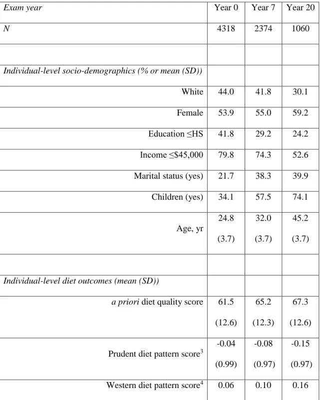
and count of food outlet.……… 83 Table 6. Descriptive statistics for study participants over the study period:
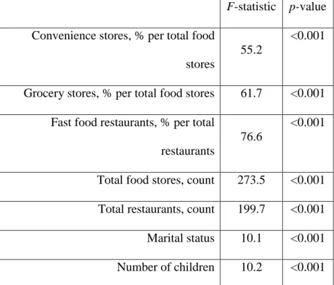
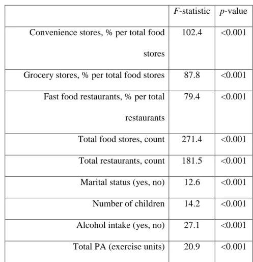
CARDIA exam years 0 (1985/86), 7 (1992/3), and 20 (2005/06)..………. 109 Table 7. F-tests (p-value) for first-stage IV regression models of
endogenous variables with a priori diet quality score: CARDIA
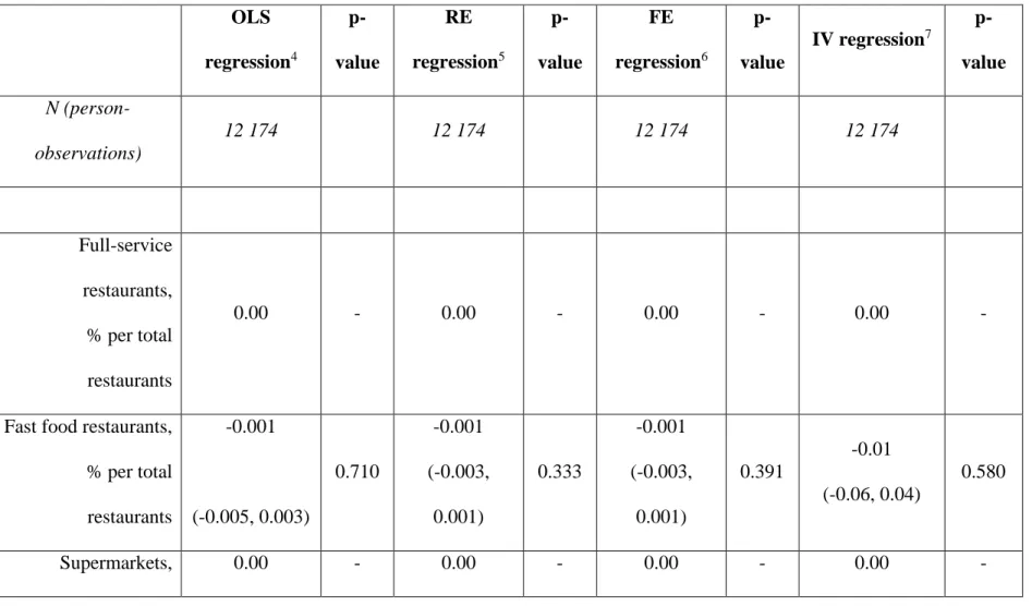
exam years 0 (1985/86), 7 (1992/3), and 20 (2005/06)..………. 112 Table 8. Beta coefficients (95% CI) for the associations between each
type of food store or restaurant and a priori diet quality score, using OLS, FE, and IV regression: CARDIA exam years 0
(1985/86), 7 (1992/3), and 20 (2005/06)..……….. .113 Supplemental Table 3. Beta coefficients (95% CI) for the associations
between each type of food store or restaurant and diet outcomes, using IV regression: CARDIA exam years 0 (1985/86), 7
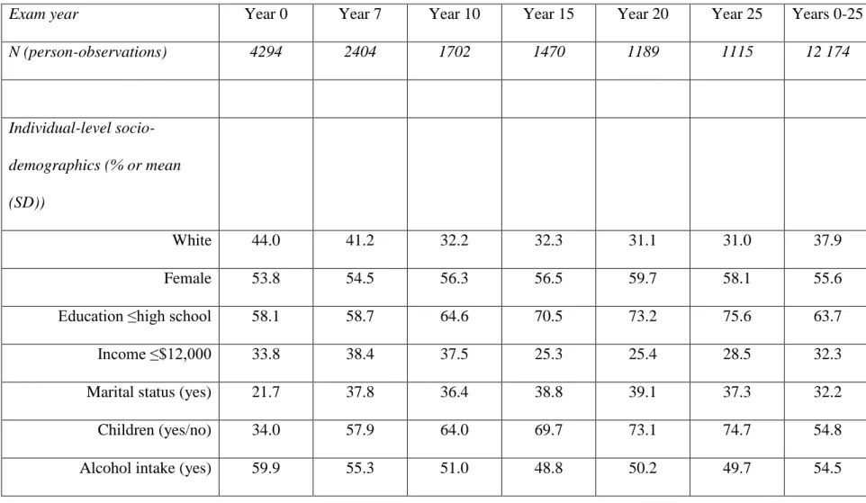
Table 9. Descriptive statistics for study participants over the study period:
CARDIA exam years 0-25 (1985/86-2010/11)…...……….132 Table 10. F-tests (p-value) for first-stage IV regression models of
endogenous variables with BMI: CARDIA exam years 0-25
(1985/86-2010/11).……….. 135 Table 11. Beta coefficients (95% CI) for the associations between each
type of food store or restaurant and BMI, using OLS, FE, and
IV regression: CARDIA exam years 0-25 (1985/86-2010/11)..……….. 136 Supplemental Table 4. Beta coefficients (95% CI) for the associations
between each type of food store or restaurant and WC, using OLS, FE, and IV regression: CARDIA exam years 0-25
(1985/86-2010/11)..………..………... 139 Supplemental Table 5. F-tests (p-value) for first-stage IV regression
models of endogenous variables with WC: CARDIA exam
LIST OF FIGURES
LIST OF ABBREVIATIONS
ACS American Community Survey
AL Alabama
BMI Body mass index
C2ER Community and Economic Research
CA California
CARDIA Coronary Artery Risk Development in Young Adults CBSA Core Based Statistical Area
CI Confidence interval CPI Consumer Price Index
CTPP Census Transportation Planning Package D&B Dun & Bradstreet
FE Fixed effects
FIML Full-information maximum likelihood GIS Geographic Information System GMM Generalized method of moments HPI Home Price Index
HS High school
IL Illinois
IQR Interquartile range IV Instrumental variables
MN Minnesota
OLS Ordinary least squares PA Physical activity
RE Random effects
SES Socioeconomic status SE Standard error
SD Standard deviation
SIC Standard Industrial Classification SSB Sugar-sweetened beverage TAZ Traffic Analysis Zones
US United States
CHAPTER I. INTRODUCTION Background
Although observational evidence suggests that the neighborhood food environment influences diet behavior and weight status, the findings in the existing literature are highly inconsistent. Some researchers propose that improvements to the built environment can promote healthy lifestyles and reduce cardiometabolic risk, but there are substantial challenges in
studying the influence of neighborhood factors on health. Previous research is undermined by a scarcity of longitudinal, high quality data, as well as a lack of adequate methods to address residential choice and the purposeful placement of food stores and restaurants in neighborhoods over time. Despite these limitations, intervention and policy approaches to alter food
environments are occurring at local, state, and federal levels, even though the impact of these changes is unknown.
placement of both food stores and restaurants and selective migration to locate near those stores and restaurants, and information regarding the magnitude and direction of these potential sources of bias is lacking. To strengthen causal inference, these various data and methodological
limitations must be resolved.
To address these limitations, we capitalized on 25 years of diet behavior and clinic-based, anthropometric, and biomarker data from the Coronary Artery Risk Development in Young Adults (CARDIA) study. CARDIA is a prospective study of black and white young adults followed for 25 years (n=5,115; aged 18-30 at baseline, 1985-86). We also used detailed, time-varying individual-level diet, anthropometric, and sociodemographic data, as well as
neighborhood-level data related to neighborhood-level food outlet locations, transportation infrastructure, housing price indices, sociodemographics, and employment sub-centers in the four CARDIA baseline cities: Birmingham, Chicago, Minneapolis, and Oakland.
Using these unique data, we sought to examine how residential locational choice relates to the food environment and physical activity opportunities, and how neighborhood
sociodemographic characteristics and the pre-existing food environment influence the
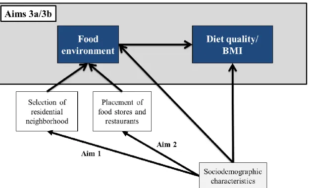
Specific aims
The primary goal of this research was to use a causal model to explicitly account for unobserved heterogeneity in longitudinal associations between the neighborhood food
environment with dietary behavior and weight status. We sought to accomplish this goal with several aims, as follows:
Aim 1: Determine how sociodemographic characteristics of individuals and their
neighborhoods are related to the neighborhood food and built environment over time. Use multinomial logistic regression to examine how individual- and neighborhood-level
sociodemographic characteristics influence the distribution of food outlets and built environment features in residents’ neighborhoods over time, and whether these associations differ by
individual-level income.
Aim 2: Determine how neighborhood-level characteristics are associated with the density of different types of food outlets over time. Use two-step econometric models to estimate which neighborhood sociodemographic characteristics are associated with the density of fast food restaurants, full-service restaurants, convenience stores, grocery stores, and supermarkets (separately) over time, regardless of their presence in neighborhoods.
a. Use IV regression to estimate associations between the availability of fast food
restaurants, full-service restaurants, convenience stores, grocery stores, and supermarkets (separately) with a priori and empirical diet patterns over time. Compare the magnitude and direction of results to standard regression models.
b. Use IV regression to estimate associations between the availability of fast food
CHAPTER II. LITERATURE REVIEW The significance of the food environment
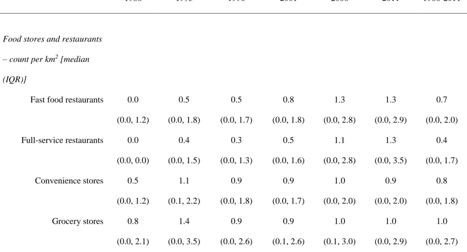
Since the 1970s, the prevalence of obesity among adults in the U.S. has more than doubled and the prevalence continues to increase [1]. Energy intake from foods obtained away from home also dramatically increased during the same period time [2-5], which may be linked to changes in the local food environment. For example, the availability of convenience stores and fast food restaurants increased between 1985 and 2006, while the availability of supermarkets and full-service restaurants remained relatively stable [6-9].
In the past decade, there has been increased attention to ‘food deserts’ (lack of healthy food options) and ‘food swamps’ (abundance of unhealthy food options) [10-12]. The literature has shown that the unequal distribution of food outlets plays a role in shaping dietary behaviors and weight status, possibly through differences in the availability of ‘healthy’ or ‘unhealthy’ foods across different types of food outlets [13, 14]. Several observational studies have shown that a higher availability of neighborhood fast food restaurants, convenience stores, and grocery stores is associated with less healthy dietary behaviors and higher BMI [6, 13, 15-19]. The literature also suggests that a higher availability of neighborhood supermarkets and full-service restaurants is associated with better dietary outcomes and lower BMI [13, 14, 18-22]. However, other studies report weak or no associations between the neighborhood food environment with diet and obesity outcomes [8, 15, 23-25].
placement of food outlets over time, as well as a lack of longitudinal, high quality data related to the neighborhood food environment, diet, and weight status. In the following sections, each of these gaps is discussed in detail.
Importance of accounting for residential self-selection
A major limitation in the food environment literature is potential bias due to residential self-selection. Residential self-selection bias occurs because the selective choice to reside in a neighborhood can be directly and indirectly related to food environment exposures and diet and weight outcomes, which induces confounding in associations between the neighborhood food environment and health outcomes. For example, previous studies have reported that residential location choice and residential preference are both positively associated with the number of and proximity to retail and PA facilities [26-29]. For example, proximity of grocery stores had a positive impact on stated residential preferences among individuals living in Belgium [30]. The literature also suggests that individuals’ self-reported residential preferences are influenced by individual- and neighborhood level sociodemographics, proximity to employment subcenters, and affordability [29, 31-36], among many other factors. However, there is little research examining relationships between actual residential location choice and the neighborhood food environment.
improve their diet quality (and vice-versa for those locating far from ‘healthy’ food outlets), thus magnifying the association between the food environment and health outcomes. It is also
possible that a mismatch exists between the demand and availability of certain types of food outlets (e.g., high demand for fast food meals among individuals locating in neighborhoods with few fast food restaurants), which would bias associations toward the null.
If individuals choose or are constrained to locate in neighborhoods with certain diet-related amenities, then the allocation of individuals to food environments is not random and observational studies of neighborhood associations with diet and weight outcomes will be biased [37]. More research is needed to understand and describe the systematic differences in the characteristics of individuals who choose certain food environments. Such work can inform whether complex modeling approaches are required to account for unobserved heterogeneity in location decisions and to support causal inference in the context of neighborhood food
environment studies. Future research can also be used to generate hypotheses about the direction and magnitude of bias due to selective residential location choice in observational research of neighborhood effects on diet and obesity outcomes.
Importance of accounting for purposeful food resources placement
In addition to residential location choice, the establishment of food stores and restaurants occurs purposefully. According to a rich evidence base in urban economics, the most important factors that influence food retail site selection include a high density of existing food outlets, zoning ordinances, competition levels, proximity to complementary businesses, cost
the central business district [43]. Furthermore, the literature suggests that food stores and restaurants are less likely to be placed in neighborhoods of low SES and high minority populations, but results are not always consistent [45] and may differ by type of outlet [46].
Despite this evidence, the majority of research on the neighborhood food environment and health outcomes has assumed that food stores and restaurants are randomly allocated across social and geographic space, and thus these studies ignore potential bias due to purposeful placement of food resources. Purposeful placement of food stores and restaurants has been previously unmeasured in the food environment literature, and introduces bias if the factors related to food store and restaurant placement are directly or indirectly associated with the
exposure (e.g., availability of food stores and restaurants) and the outcomes (e.g., diet quality and weight status). For example, several studies have shown that methods that do not account for non-random exposure to programs and services, such as child care facilities [47], family health services [48], and family planning clinics [49], may underestimate the benefits of these programs and services (e.g., contraceptive use).
The literature is lacking studies that quantify heterogeneity in the placement of different types of food stores and restaurants over time, and specifically how neighborhood
Where do people shop?
Even if food outlets are available within individuals’ residential neighborhoods, consumers may travel to purchase food items or meals farther away (i.e., potential vs. realized access) [50, 51]. A number of studies have reported that consumers did the majority of their shopping at
supermarkets outside of their residential neighborhood [52-55], with key differences by car ownership, education, and income [56, 57]. Traveling outside of residential neighborhoods to access food outlets might increase the likelihood of finding null effects of the residential food environment on health outcomes. Therefore, it is important to account for unmeasured
confounding in neighborhood food environment research, especially if we hypothesize that unobserved heterogeneity will bias neighborhood effects on diet and obesity outcomes toward the null.
The need for causal models of neighborhood effects on health outcomes
The literature examining associations between the neighborhood food environment, diet, and weight status is predominately cross-sectional [58, 59], with several studies using ordinary least squares (OLS) regression [5, 18, 60]. OLS regression may generate biased estimates if omitted variables, such as residential self-selection or the purposeful placement of food stores and restaurants, influence food environment exposures and health outcomes [61]. Other sources of endogeneity may bias estimates of neighborhood effects in OLS models, such as differential measurement error (e.g., higher rate misclassification of food environment exposures in low-income areas) or reverse causality (e.g., dietary behavior or weight status influencing
confounding, differential measurement error, and reverse causality do not exist, and thus may magnify or underestimate associations between the neighborhood food environment and health outcomes [61]. Estimates of neighborhood effects in the literature are often weak, so ignoring these potential sources of bias could impact the accuracy of reported associations, particularly if the bias is towards the null.
Despite the largely cross-sectional literature, several studies have utilized analytic approaches that maximize longitudinal data, such as repeated-measures random effects (RE) regression and fixed effects (FE) regression. RE regression is vulnerable to the same type of biases as OLS regression, and does not account for time-invariant or time-varying unmeasured characteristics [61]. Alternatively, FE regression models quantify within-person associations and control for all measured and unmeasured time-invariant characteristics, effectively using each individual as his/her own control [61]. For example, a previous study found that higher
availability of neighborhood grocery stores was positively associated with diet quality using RE regression over 15 years in the CARDIA study; however, the association was strongly attenuated using FE regression [58]. Although this study suggests that controlling for unmeasured
characteristics is critical in neighborhood food environment studies, FE regression models do not account for unmeasured characteristics that change over time (e.g., time-varying residential location preferences) [61], which may further bias estimates.
Although the literature suggests that unmeasured residential preferences may change over time [62], few studies have examined the extent to which time-variant and time-varying
the correlation between food environment exposures and unmeasured characteristics (e.g., selective residential location choice). To provide valid causal effects, it is assumed and
empirically tested that instrumental variables are directly associated with the exposures but not with the outcome (outside of their association with the exposures), and independent of the error terms in the model. With correct model specification and strong identification of endogenous variables, IV regression theoretically provides less biased estimates because less advanced analytic approaches due not account for the presence of time-varying sources of unobserved heterogeneity. The presence and extent of bias can also be evaluated with IV regression by comparing estimates to those derived from less complex models (e.g., OLS regression).
For example, a few studies have used IV regression with cross-sectional data to estimate associations between the availability of fast food restaurants and BMI, and compared results to OLS regression [66-68]. These studies found that the associations between fast food restaurants and BMI were smaller in magnitude using OLS regression than IV regression. However, cross-sectional studies by design ignore temporal changes in diet and health outcomes over time, especially in the critical lifecycle period of late adolescence to middle adulthood when poor dietary behaviors and weight increase [69]. Longitudinal data are important because
with diet behavior data, or examined similar associations with convenience stores and supermarkets/grocery stores. A previous study used IV regression with longitudinal data to examine the effect of Walmart Supercenter locations on weight status in Bentonville, Arkansas, and the findings indicated that additional Supercenters increased BMI and the obesity rate over time; however, the authors did not compare results to standard regression models [72].
Other approaches to correct for unmeasured confounding
There are other methods to control for bias commonly used in epidemiologic studies, such as inverse probability weighting and propensity score matching, which allow for causal contrasts based on counterfactuals. Inverse probability weighting quantifies the probability of a person being sampled and assigns a weight relative to its inverse probability [73]; whereas, propensity score matching quantifies the probability that a person is exposed given his/her observed covariates, and uses this information to ‘randomize’ treatment assignment [74]. However, IV regression is the only causal model strategy that explicitly accounts for bias due to unobserved heterogeneity in observational research, whereas inverse probability weighting and propensity score matching assume that all differences between participants have been observed.
activity). This method is has also been shown to perform better than single-equation IV estimators even in the presence of weak instruments [48, 77].
Evaluations of interventions and policy changes to the neighborhood food environment In addition to observational research, a few studies have evaluated interventions and policy changes to the neighborhood food environment with natural and quasi-experimental designs [78-81]. In these studies, changes in diet and weight outcomes are compared within the same population before and after an intervention or policy change to the neighborhood food environment [82]. For example, Cummins et al conducted a pilot study to evaluate the impact of opening a new supermarket in a low income, predominately black neighborhood in Philadelphia on self-reported fruit and vegetable intake and BMI, and found that diet and weight outcomes did not change [78]. Similarly, the RAND Corporation evaluated the impact of a zoning regulation that restricted the opening or remodeling of fast-food restaurants in South Los Angeles and found that fast food consumption and overweight/obesity rates increased from 2007 to 2011/2012 [83]. Evaluations of food retail interventions in underserved areas of Michigan and the United
Kingdom have also reported a lack of change in diet outcomes [79-81]. Current and past
Conclusion
To date, small-scale, food retail-based interventions have only focused on single food outlet types in single neighborhoods, with little success in improving diets or reducing obesity [78-81, 85]. To better inform future efforts to change the retail food environment, various data and methodological limitations in observational food environment research must be resolved. In addition to a lack of longitudinal, high-quality data related to the neighborhood food
environment and diet and obesity outcomes, the literature is also lacking studies that use causal models that account for potential bias due to unobserved heterogeneity.
CHAPTER III. METHODS Study population and data sources
The CARDIA study
CARDIA is a prospective study of the development and determinants of cardiometabolic outcomes in a sample of young adults. In 1985-86, 5,115 men and women aged 18-30 years were recruited from four U.S. metropolitan field centers (Birmingham, AL; Chicago, IL; Minneapolis, MN; Oakland, CA), with approximately equal enrollment by age (18-24 y, 25-30 y), race (black, white), gender, and education [high school (HS) or less, more than HS]. Follow-up examinations were conducted in 1987-1988 (Year 2), 1990-1991 (Year 5), 1992-1993 (Year 7), 1995-1996 (Year 10), 2000-2001 (Year 15), 2005–2006 (Year 20), and 2010-2011 (Year 25), with participant retention of 91%, 86%, 81%, 79%, 74%, 72%, and 72%, respectively.
Using a Geographic Information System (GIS), we geographically- and temporally-matched neighborhood food stores and restaurants, housing and food prices, built environment features, and US Census data to CARDIA respondents’ residential addresses at baseline and exam years 7, 10, 15, 20, and 25.
U.S. Census sociodemographics
We used Census data from 1980, 1990, and 2000, and American Community Survey (ACS) 5-year estimates from 2005–2009 and 2007–2011, that have been normalized to CARDIA respondents’ neighborhood boundaries. To match the analytic exam years, we estimated a
continuous change in sociodemographic characteristics across all decennial and quinquennial censuses using linear interpolation.
Employment subcenters
Using employment data from the Census Transportation Planning Package, we identified employment subcenters in each of the four baseline field centers. Any contiguous group of Traffic Analysis Zones (TAZs) that met our threshold criterion [33] were collapsed into an employment subcenter, defined as a region of significant employment density.
Street connectivity
C2ER food prices
Since 1968, the Council for Community and Economic Research (C2ER, formerly known as the American Chamber of Commerce Research Association) has collected price data quarterly from over 300 urban areas in the U.S., including participation by federally designated Core Based Statistical Areas (CBSAs), as well as cities in non-metropolitan counties with a county population >50,000 and a city population >35,000. The C2ER uses these price data to derive a county-level cost of living index, which is the industry standard for comparing costs of living in cities across the U.S. (https://www.coli.org/store.asp).
Data collectors for the C2ER gather prices on 60 consumer goods and services from six major categories: grocery items, housing, utilities, transportation, health care, and miscellaneous goods and services. Each item in the miscellaneous goods and services category is usually gathered by price collectors at a minimum of five establishments, although the minimum is three establishments in non-metropolitan areas and as many as 10 in larger metropolitan areas. Within this category, food price data is collected for 24 foods purchased for at-home consumption and 3 away-from-home foods. Specifically, price collectors report the average price of a McDonald’s Quarter-Pounder with cheese; the average price of an 11"-12" thin crust regular cheese pizza (no extra cheese) at Pizza Hut and/or Pizza Inn; and the average price of a fried chicken drumstick and thigh at Kentucky Fried Chicken and/or Church’s Fried Chicken.
were inflated to corresponding quarterly exam year dollars using the Consumer Price Index (CPI), using a 1982-84 reference base (CPI=1.0).
Using the lowest geographic level provided by C2ER (county or CBSA), we merged C2ER data to individuals by their residential location and by quarter corresponding to the CARDIA exam year when participants were seen in the clinic. Although CARDIA participants were recruited from 4 U.S. cities at baseline (Birmingham, AL; Chicago, IL; Minneapolis, MN; Oakland, CA), residential mobility at subsequent exam years necessitated imputation of prices for individuals for whom there was not a direct match between residential location and
county/CBSA (geographic entities that consist of one or more counties containing the core urban area, as well as any adjacent counties that are socially and economically integrated with the urban core) or quarter in which price data were collected. If a participant’s residential location did not have matching county- or CBSA-level data (20% of respondents across all exam years), we derived population-weighted state-level means from all C2ER-reporting cities within the participant’s state; no price data we assigned to the participants if no match was available at any geographic level. If an exact match was not available by both exam year and quarter, matching was done with prior quarters of price data, up to 1 year before the respondents' exam dates.
Cigarette prices
Housing prices
We calculated the average of quarterly values for housing price index (HPI) in each city at each exam year using values from Moody's Analytics [87]. Moody’s provides Case-Schiller real price data for Chicago, Minneapolis, and Oakland for each quarter of each year from 1975-2012 relative to a value of 100 for the first quarter of the year 2000. Moody’s provides Lender Processing Service data for Birmingham at the zip code level for each quarter from 1991-2012, measured in the thousands of dollars. We used multilevel mixed-effects linear regression (-mixed- in Stata 14.0) to predict HPI values for 1985 in Birmingham.
Analytic variables
Dietary assessment
CARDIA food and beverage groups
a priori diet quality score
We re-created an a priori diet quality score using an approach previously established by CARDIA investigators [88-90]. Briefly, based on their hypothesized relationships with health, we classified food groups as beneficial (n=20), adverse (n=13), or neutral (n=13). At each exam year, consumption (servings/week) of non-neutral foods was categorized into quintiles ranging from lowest to highest consumption and then given a score of 0 to 4 for beneficial food groups and 4 to 0 for adverse food groups; for example, intake in the highest quintile of positively-rated foods received a score of 4 and vice-versa for negatively-rated foods. For food groups with a large proportion of non-consumption, we categorized non-consumers as 0 and created quintiles for consumers only. A higher score indicates higher diet quality.
“Prudent” and “Western” diet pattern scores
Using principle components analysis with orthogonal rotation, we derived two
uncorrelated dietary patterns with the 46 food groups: one with high factor loadings of healthier foods, labeled “Prudent,” and another with high factor loadings of unhealthier foods, labeled “Western”.
Weight outcomes
Individual-level covariates
Individual-level covariates included age (continuous), age-squared, race (black, white), gender, educational attainment (HS or less, more than HS) or current educational attainment (years), marital status (yes/no), alcohol intake (yes/no), and number of children. Income (categorical responses) was collected at exam years 5, 7, 10, 15, 20 and 25; we used income values from exam year 5 as a proxy for baseline values (no other data from exam year 5 were used).
Based on previously-established methods [91], we re-created total PA intensity scores (exercise units) using a summary of the frequency and intensity of participants’ moderate and vigorous activities.
Neighborhood food environment
For each neighborhood unit in the four cities, we calculated counts the count per km2 of fast food restaurants, full-service restaurants, convenience stores, grocery stores, supermarkets, and all other types of food outlets (separately).
Prediction of full-service restaurants at baseline
The magnitude of the count of full-service food restaurants at baseline in the Dun & Bradstreet (D&B) Duns Market Identifiers File (Dun & Bradstreet, Inc., Short Hills, NJ) was inconsistent with the magnitude of the count of full-service food restaurants at later CARDIA exam years. Therefore, we used a linear mixed-effects regression model with the -mixed- command (Stata, version 14.0) to predict the count of full-service restaurants at exam year 0 only. Specifically, we specified the outcome as the time-varying count of full-service restaurants within a 1-km network-based buffer, with missing values for year 0. The covariates (exposures) used for the prediction included baseline study center and individual-level age, gender, and race; and time-varying count of fast food restaurants, count of away-from-home eating places (a combination of quick- and slow-service restaurants), population per km2, and CARDIA exam year. We set all negative predicted values to zero, and all other values were rounded to the nearest whole number. We replaced missing values for the count of full-service restaurants at exam year 0 with the predicted values derived from the linear mixed-effects regression model, and retained the original values for the count of full-service restaurants for exam years 7 and 20.
Neighborhood-level covariates
Neighborhood socioeconomic deprivation score
Cluster analysis to derive neighborhood types
To create a posteriori neighborhood clusters, we used the count of food outlets and PA facilities within each neighborhood (per km2); the distance from each neighborhood centroid to the nearest employment center centroid; variables related to road types and lengths; and total park area (km2). We transformed all calculated variables used to define neighborhood clusters into z-scores and used the PROC FASTCLUS procedure in SAS (version 9.3) to conduct non-hierarchical cluster analysis using means of these standardized variables at each exam year. Our final cluster solution included 3 distinct clusters, with neighborhoods assigned to clusters with low, average, and high road connectivity and activity- and diet-related amenities, respectively.
Inverse probability weights
CHAPTER IV. HOW DO INDIVIDUAL- AND NEIGHBORHOOD-LEVEL SOCIODEMOGRAPHICS INFLUENCE RESIDENTIAL LOCATION BEHAVIOR IN
THE CONTEXT OF THE FOOD AND BUILT ENVIRONMENT?
Overview
Little is known about how diet and activity-related amenities relate to residential location behavior. Understanding these relationships is essential for addressing residential self-selection bias.
Using 25 years (6 exams) of data from the CARDIA study (n=11,013 observations) and linked neighborhood-level data from the four CARDIA baseline cities (Birmingham, AL; Chicago, IL; Minneapolis, MN; Oakland, CA), we characterized participants’ neighborhoods as having low, average, or high road connectivity and amenities using non-hierarchical cluster analysis. We then used repeated measures multinomial logistic regression with random effects to examine the associations between individual- and neighborhood-level sociodemographic
characteristics and residential neighborhood types over the 25 year period, and whether these associations differed by individual-level income.
low (vs. high) connectivity and amenities. Housing price did not influence residential location behavior related to neighborhood connectivity and amenities at any income level.
Our study is an important step in understanding how residential locational behavior relates to amenities and PA opportunities, and may help mitigate residential self-selection bias in built environment studies.
Introduction
A primary challenge of neighborhood health research is that it is difficult to tease apart the influence of the neighborhood on its residents from the fact that residents choose their neighborhoods on the basis of health-related amenities. If unaccounted for, neighborhood selection factors may bias associations of built environment factors and health outcomes. Therefore, to address potential residential self-selection bias it is important to understand how access to health-related amenities influences residential behavior.
The few studies that have addressed how diet and activity-related amenities relate to residential location behavior have found a positive association between residential location with proximity and number of retail and physical activity (PA) facilities [26-28]. There are also examples of reported preferences for living in neighborhoods with lower intersection density and street networks [27, 31, 94], despite positive observed associations between road connectivity and PA [95].
(vs. actual location behavior), with limited geographic generalizability. Furthermore, little is known about how the relationship between diet and activity-related amenities and residential location behavior varies by individual-level income.
Using 25 years of time-varying data from CARDIA study with linked neighborhood-level data from four U.S. cities, we sought to fill these gaps. We used repeated measures to estimate average associations between individual- and neighborhood-level sociodemographic
characteristics of CARDIA participants with neighborhood food- and activity-related amenities and infrastructure over the 25 year period. Because income is a major factor in residential location behavior [31], we hypothesized that these associations would differ by individual-level income.
Methods Study sample
CARDIA is a prospective study of the development and determinants of cardiometabolic outcomes in a sample of young adults. In 1985-86, 5,115 men and women aged 18-30 years were recruited from four U.S. metropolitan field centers (Birmingham, AL; Chicago, IL; Minneapolis, MN; Oakland, CA), with approximately equal enrollment by age (18-24 y, 25-30 y), race (black, white), gender, and education (HS or less, more than HS). Follow-up examinations were
years 7, 10, 15, 20, and 25. Using a GIS, we geographically- and temporally-matched neighborhood-level data to participants’ residential locations.
We defined neighborhoods using socially-constructed boundaries from Zillow [86] where available (Chicago, IL; Oakland, CA; Minneapolis, MN) and the Regional Planning Commission of Greater Birmingham (Birmingham, AL), for a total of 392 neighborhoods at each exam year (2,352 observations). Therefore, our analytic sample only included participants who remained in the four baseline cities at any given exam year, with a total of 4,314, 2,461, 1,727, 1,480, 1,202, and 1,119 participants at baseline and exam years 7, 10, 15, 20, and 25, respectively.
Cluster analysis to derive neighborhood types
Our baseline sample of CARDIA individuals was geographically clustered due to targeted enrollment by age, gender, race, and education, thus there were neighborhoods in the 4 cities with zero or few participants. Therefore, we created a posteriori neighborhood clusters using non-hierarchical cluster analysis to characterize neighborhoods where sufficient numbers of individuals lived.
To capture aspects of the neighborhood environment related to diet and PA, we created variables using data from several commercial data sets (Table 1). We calculated the count of food outlets and PA facilities within each neighborhood (per km2) at each exam year using data from D&B [96]. We classified food outlets and PA facilities according to 8-digit Standard Industrial Classification (SIC) codes, except in 1986 when only 4-digit codes were available, which were used along with matched business names. We used data from the Census
0, 7, 10), 2000, 2005, and 2010 (exam years 15, 20, and 25, respectively); we defined
employment centers as regions of significant employment density with any contiguous group of TAZs that met our threshold criterion [33]. We extracted data from StreetMap Pro datasets to create variables related to road types and lengths for each neighborhood in 1999 (exam years 0, 7, 10, 15), 2005 and 2010 (exam years 20 and 25, respectively). We also collected total park area (km2) using current and historic geospatial data at each exam year. We transformed all calculated variables used to define neighborhood clusters into z-scores to achieve more comparability across measures (Table 2).
Using the PROC FASTCLUS procedure in SAS (version 9.3), we conducted cluster analyses using means of these standardized variables at each exam year and a range of 2 to 6 clusters. To determine a final cluster solution, we evaluated the distribution of individuals across clusters; differences in proportions across clusters; parsimony; and meaningfulness of clusters. We classified values ≥0.5 or ≤-0.50 as high or low, respectively [97]. We also evaluated whether clusters appeared repeatedly across solutions (robustness) by performing the cluster analysis many times. After determining the appropriate number of clusters from this step, we performed 1000 iterations of the cluster analysis using a SAS macro, which identified the cluster solution with the highest R2 value; we used this categorical variable of neighborhood type as our outcome.
Neighborhood-level exposures
estimates from 2005–2009 and 2007–2011 (when comparable US Census data were unavailable). Using linear interpolation, we estimated a continuous change in sociodemographic
characteristics across the full period of the decennial and quinquennial censuses. We also derived a neighborhood socioeconomic deprivation score using principal components analysis of: (1) percentage of population with less than HS education at age 25; (2) percentage of population with at least a college degree at age 25; (3) median household income; and (4) percentage of population with household income less than 150% of federal poverty level [93]; a higher score indicates higher neighborhood socioeconomic deprivation.
We calculated the average of quarterly values for HPI in each city at each exam year using values from Moody's Analytics [87]. Moody’s provides Case-Schiller price data for Chicago, Minneapolis, and Oakland for each quarter of each year from 1975-2012 relative to a value of 100 for the first quarter of the year 2000. Moody’s provides Lender Processing Service data for Birmingham at the zip code level for each quarter from 1991-2012, measured in the thousands of dollars. We used multilevel mixed-effects linear regression (-mixed- in Stata 13.0) to predict HPI values for 1985 in Birmingham.
Given that neighborhood-level variables were available at different geographic levels, we harmonized all variables (including those used to define neighborhood cluster types) to fit our socially-constructed neighborhood boundaries within city limits. We also created a
Individual-level exposures
We also adjusted for several individual-level sociodemographic confounders. At each CARDIA exam year, a standardized questionnaire was used to collect self-reported individual-level sociodemographic characteristics, including age, gender, race, and current educational attainment (highest grade or year of school completed). Income was collected with categorical responses at exam years 5, 7, 10, 15, 20 and 25; we substituted income values from exam year 5 for baseline values, which were unavailable.
Statistical analysis
We used repeated measures multinomial logistic regression with random effects to examine the associations between individual- and neighborhood-level characteristics with the neighborhood type that each participant chose at each time period; thus, model estimates represent the average difference in neighborhood cluster type between individuals at each cross-section of time over the 25 year period . Our individual-level exposures included age
(continuous), race (black, white), gender, and education (HS or less, more than HS); and our neighborhood-level exposures included socioeconomic deprivation score, percentage of non-Hispanic white population, and percentage of the population ≤18 years. We also adjusted for exam year and study center. Based on evidence showing that model estimates may improve with interaction terms for income groups [29], we stratified our analyses by tertiles of individual-level income (coded as the midpoint of the categorical response).
command for testing the equality of coefficients across tertiles of individual-level income; we accounted for clustering by neighborhood ID using the ‘cluster’ option. We also used the
-margins- post-estimation command with the -predict- option to predict the probability of residing in each neighborhood cluster type at fixed levels of the covariates [categories or +/-1 standard deviation (SD) of mean].
To account for potential selection bias due to out-migration from the four cities over time, we used a probit model to derive inverse probability weights. We used gender, race, and baseline study center to predict the probability of being in the sample at Year 25, and used the inverse of the probability to weight the models in the central analysis (-pweight-); interaction terms among covariates in the probit model were not statistically significant, and therefore were not included in the final model.
Given empirical evidence of the importance of housing price in residential behavior [29], we ran two separate models: a model with neighborhood clusters stratified by high and low HPI (< and ≥50th percentile, respectively) and a model with non-stratified clusters. We used a likelihood-ratio test to assess the fit of these two models.
Results
count of road links, and beta index, with a higher count of PA facilities and all food outlets; a lower percentage of local roads and closer proximity to employment subcenters. The fit of the model with fewer clusters was statistically significantly better than the model with clusters divided by high/low HPI (p<0.05); thus, we included HPI as a covariate rather than stratify clusters in the final model.
Among low-income participants, individual-level race, gender, educational attainment, and age were not statistically significantly associated with any of our derived residential clusters over time, although there were statistically significant differences among high-income
participants (Supplemental Table 1). Within the high-income tertile, the probability of residing in a neighborhood with low (vs. high) road connectivity and activity- and diet-related amenities was lower for white (vs. black) participants and higher for females (vs. males) (Table 3). Similarly, the probability of residing in the low (vs. high) connectivity/amenities cluster was higher for older (vs. younger) participants.
The probability of residing in a neighborhood with low (vs. high) road connectivity and activity- and diet-related amenities was higher in neighborhoods with a higher (vs. lower) deprivation score among both low- and high-income participants (Table 3). Conversely, the probability was lower in neighborhoods with a higher (vs. lower) percentage of neighborhood population ≤18 years among both low- and high-income participants. Regardless of income level, we did not observe statistically significant associations between the percentage of neighborhood white population and neighborhood cluster type, nor between HPI and neighborhood cluster type.
Overall, findings for medium-income participants were similar to low-income
low (vs. high) connectivity/amenities cluster was lower for individuals with higher educational attainment among medium-income participants, but not those at low or high income levels.
Discussion
Using 25 years of retail and built environment data, we examined the relationship between individual- and neighborhood-level sociodemographic characteristics and living in activity-supportive, commercially-dense neighborhoods over time, and whether these
associations differed by individual-level income. We found that individual-level race, age, and gender and the percentage of neighborhood white population were associated with residential location among high-income CARDIA participants, but not among low- and medium-income participants. Neighborhood-level SES and age composition were also related to residential location behavior at all income levels.
White (vs. nonwhite) race is negatively related to preferences for walkable
more compact neighborhoods [35]. However, high-income women may be able to afford to own a car and drive to destinations, and thus may choose to reside in less urban areas [98].
As neighborhood deprivation increased, individuals of all income levels were less likely to locate in neighborhoods with low (vs. high) road connectivity and activity- and diet-related amenities. Despite a preference to reside in walkable and commercially-dense neighborhoods, individuals in our cohort may be adverse to locating in low SES neighborhoods (which may be proxies for poorer housing quality or higher crime and unemployment) and rather locate in less deprived areas with low connectivity and amenities [29]. Similarly, individuals in our cohort were more likely to reside in neighborhoods with low (vs. high) connectivity/amenities as the percentage of population <18 years increased. Thus, it appears that neighborhood age
composition affects selection into walkable, commercially-dense neighborhoods for individuals at all ages and income levels; whereas, an individual’s own age affects selection into
neighborhoods with high connectivity/amenities among high-income individuals only. This finding is supported by several studies that show that households with school-age children tend to live in less densely-populated areas [99], and prefer to locate near other households with families [29]. It is also possible that associations between neighborhood SES and age
composition with residential location behavior differed by individual-level income level, but the magnitude of estimated effect may have been too small to detect in our sample.
have accurately reflected the housing market for low-income individuals, who are more likely to rent residential property.
Overall, our findings suggest that individual-level income may modify associations between individual-level sociodemographics and residential location related to walkability and activity- and diet-related amenities. High-income individuals may be able to choose
neighborhoods based on preferences for connectivity and access to amenities, whereas low-income individuals may not have sufficient low-income to actualize their preferences. Based on these preferences, our findings also suggest that residential location behavior may bias estimates of the relationship between the physical environment and health outcomes. Hypothetically, individuals living in neighborhoods with greater PA opportunities are more likely to be physically active, and individuals who live in areas with a high density of eating-out options may have poorer dietary behaviors.
Studies that examine the influence of the food and built environment on residential location behavior are mostly based on self-reported preference surveys [26, 30] and
cross-sectional data [26, 30, 100]. In contrast, we had access to detailed, time-varying measures, which allowed us to use information both within and between participants, thus producing more
adjust for population density due to collinearity with our explanatory variables. Finally, we did not know the extent to which participants are constrained to live in areas due to observed or unobserved factors (e.g., discrimination); however, stratifying our models by individual-level income may have mitigated constraints related to affordability. Future options for addressing unmeasured neighborhood selection factors include complex modeling of residential behavior or longitudinal analytic approaches that maximize panel data, such as regression with lagged variables.
Conclusion
38
Tables and figures
Table 1. Descriptive statistics of raw means and medians by neighborhood cluster a type, pooled cities & CARDIA Exam Years 0-25
MEANS (SD)
Links (count) c 670 (666) 229 (194) 502 (378)
Cul-de-sacs (count) 21.0 (14.9) 8.1 (8.7) 15.5 (11.4)
Beta index d 1.9 (0.2) 2.0 (0.3) 2.1 (0.5)
Total road length (km) 110,981 (94,995) 32,499 (31,526) 66,707 (49,592)
Percentage residential e 74.8 (9.3) 77.6 (9.6) 68.9 (10.4)
Distance to nearest employment sub-center f 6,895 (3,722) 5,420 (2,804) 3,010 (1,977)
PA facilities (count) 20.8 (23.5) 5.8 (9.5) 32.8 (43.9)
Fast food restaurants (chain) (count) 3.2 (4.1) 0.6 (1.2) 3.7 (4.1)
39
Full-service restaurants (count per km2) 0.5 (0.8) 0.8 (1.4) 5.1 (7.7)
Supermarkets (count) 1.0 (1.5) 0.3 (0.9) 1.0 (1.7)
Co-ops (count) 0.1 (0.3) 0.1 (0.4) 1.3 (1.6)
MEDIAN (IQR)
PA facilities (count per km2) 1.8 (0.7-2.7) 1.8 (0.7-3.4) 4.5 (1.8-8.6) Fast food restaurants (chain) (count per km2) 0.2 (0.0-0.5) 0.0 (0.0-0.3) 0.7 (0.2-1.3) Full-service restaurants (count per km2) 0.0 (0.0-1.1) 0.0 (0.0-1.0) 0.1 (0.9-7.7) Convenience stores (count per km2) 0.7 (0.3-1.3) 0.9 (0.3-1.7) 1.9 (1.1-3.1) Supermarkets (count per km2) 0.0 (0.0-0.1) 0.0 (0.0-0.0) 0.0 (0.0-0.3) Co-ops (count per km2) 0.0 (0.0-0.1) 0.0 (0.0-0.0) 0.1 (0.0-0.5)
a Clusters created a posteriori clusters using non-hierarchical cluster analysis with 392 neighborhoods across 6 exam years (n=2352 neighborhoods) in the core 4 cities (Birmingham, AL; Chicago, IL; Minneapolis, MN; Oakland, CA)
40
d Ratio of links to nodes (intersections) e Percentage of roads used for local traffic
41
Table 2. Descriptive statistics of z-score means by neighborhood cluster type a, pooled cities & CARDIA Exam Years 0-25 Low connectivity/
amenities cluster [n=545 (23.2%)]
Average connectivity/ amenities cluster [n=409 (17.4%)]
High connectivity/ amenities cluster [n=1398 (59.4%)]
Intersection density b -0.92 0.21 0.66
Links (count) c 0.19 -0.20 0.62
Cul-de-sacs (count) 0.87 -0.27 -0.18
Beta index d -0.26 -0.17 1.00
Total road length (km) 0.92 -0.31 0.04
Percentage residential e -0.21 0.30 -0.76
Distance to nearest employment sub-center f
0.62 -0.05 -0.85
Total park area (km2) g 0.66 -0.25 -0.07
PA facilities h -0.50 -0.12 1.04
42
Fast food restaurants (chain) h -0.27 -0.18 0.92
Full-service restaurants h -0.32 -0.22 1.14
Supermarkets h -0.25 -0.11 0.68
Co-ops h -0.21 -0.11 0.83
a Clusters created a posteriori clusters using non-hierarchical cluster analysis with 392 neighborhoods across 6 exam years (n=2352 neighborhoods) in the core 4 cities (Birmingham, AL; Chicago, IL; Minneapolis, MN; Oakland, CA)
b Intersection density represents the number of 3-way, 4-way, and higher intersections per km2 c Number of connections between intersections
d Ratio of links to nodes (intersections) e Percentage of roads used for local traffic
f Distance from neighborhood centroid to nearest employment center centroid (km) g Within each neighborhood (clipped)
43
Table 3. Model-estimated a multivariable-adjusted b predicted probabilities (95% CI) of residing in a neighborhood cluster c by income status and levels (categories or +/-1SD of mean) of covariates using multivariate multinomial logistic regression, CARDIA Exam Years 0-25
Low connectivity/ amenities [n=545
(23.2%)]
Average connectivity/ amenities [409
(17.4%)]
High connectivity/ amenities [1398
(59.4%)]
Low income (1st tertile)
Black 0.27 (0.18, 0.37) 0.50 (0.42, 0.59)† 0.23 (0.17, 0.28) White 0.29 (0.18, 0.39) 0.54 (0.44, 0.63)† 0.18 (0.13, 0.23)
Female 0.21 (0.17, 0.26) 0.27 (0.18, 0.37) 0.51 (0.42, 0.59) Male 0.21 (0.16, 0.26) 0.28 (0.18, 0.37) 0.52 (0.43, 0.61)
44
Education ≥ HS 0.28 (0.18, 0.37) 0.51 (0.43, 0.59) 0.21 (0.16, 0.26)
Age (y) (-1SD) 0.26 (0.17, 0.36) 0.54 (0.45, 0.63) 0.20 (0.15, 0.25) Age (y) (+1SD) 0.29 (0.19, 0.40) 0.48 (0.37, 0.58) 0.23 (0.17, 0.30)
Neighborhood deprivation score (-1SD) 0.20 (0.12, 0.28)* 0.49 (0.39, 0.58)† 0.31 (0.24, 0.38) Neighborhood deprivation score (+1SD) 0.50 (0.33, 0.67)* 0.39 (0.22, 0.56)† 0.11 (0.07, 0.15)
Percentage white population (-1SD) 0.24 (0.09, 0.40) 0.54 (0.38, 0.70) 0.21 (0.13, 0.30) Percentage white population (+1SD) 0.29 (0.13, 0.46) 0.50 (0.35, 0.65) 0.21 (0.13, 0.29)
Percentage population ≤18 years (-1SD) 0.47 (0.33, 0.61)* 0.49 (0.36, 0.62)† 0.04 (0.02, 0.07) Percentage population ≤18 years (+1SD) 0.07 (0.03, 0.10)* 0.36 (0.27, 0.44)† 0.58 (0.48, 0.67)
45
Medium income (2nd tertile)
Black 0.31 (0.21, 0.41) 0.50 (0.41, 0.59) 0.19 (0.15, 0.24) White 0.27 (0.17, 0.36) 0.57 (0.47, 0.66) 0.17 (0.12, 0.22)
Female 0.27 (0.18, 0.37) 0.54 (0.46, 0.63) 0.18 (0.13, 0.23) Male 0.30 (0.20, 0.40) 0.52 (0.43, 0.61) 0.18 (0.13, 0.23)
Education < HS 0.33 (0.23, 0.43)* 0.15 (0.10, 0.19) 0.52 (0.43, 0.61) Education ≥ HS 0.28 (0.18, 0.37)* 0.19 (0.14, 0.24) 0.53 (0.45, 0.62)
Age (y) (-1SD) 0.29 (0.19, 0.39) 0.52 (0.43, 0.62) 0.19 (0.14, 0.24) Age (y) (+1SD) 0.30 (0.17, 0.42) 0.54 (0.42, 0.66) 0.16 (0.10, 0.23)
46
Percentage white population (-1SD) 0.24 (0.13, 0.34) 0.60 (0.47, 0.73) 0.16 (0.11, 0.22) Percentage white population (+1SD) 0.35 (0.12, 0.57) 0.45 (0.25 , 0.64) 0.21 (0.10, 0.31)
Percentage population ≤18 years (-1SD) 0.51 (0.37, 0.66)* 0.02 (0.004, 0.04)† 0.46 (0.33, 0.60) Percentage population ≤18 years (+1SD) 0.12 (0.07, 0.17)* 0.47 (0.39, 0.55)† 0.41 (0.33, 0.49)
HPI (-1SD) 0.31 (0.18, 0.44) 0.53 (0.42, 0.65) 0.16 (0.10, 0.22) HPI (+1SD) 0.25 (0.14, 0.37) 0.52 (0.38, 0.67) 0.22 (0.11, 0.34)
High income (3rd tertile)
Black 0.36 (0.25, 0.48)* 0.42 (0.32, 0.52) 0.22 (0.16, 0.28) White 0.23 (0.16, 0.31)* 0.47 (0.39, 0.55) 0.30 (0.24, 0.35)
47
Education < HS 0.29 (0.21, 0.38) 0.46 (0.37, 0.55) 0.25 (0.19, 0.30) Education ≥ HS 0.28 (0.20, 0.35) 0.45 (0.37, 0.52) 0.27 (0.23, 0.32)
Age (y) (-1SD) 0.27 (0.18, 0.35)* 0.39 (0.31, 0.48)† 0.34 (0.28, 0.40) Age (y) (+1SD) 0.30 (0.17, 0.42)* 0.49 (0.36, 0.63)† 0.21 (0.14, 0.27)
Neighborhood deprivation score (-1SD) 0.06 (0.02, 0.11)* 0.65 (0.53, 0.77) 0.28 (0.17, 0.40) Neighborhood deprivation score (+1SD) 0.39 (0.31, 0.47)* 0.35 (0.28, 0.43) 0.26 (0.21, 0.30)
Percentage white population (-1SD) 0.23 (0.16, 0.31) 0.53 (0.45, 0.61)† 0.24 (0.20, 0.28) Percentage white population (+1SD) 0.31 (0.14, 0.48) 0.26 (0.13, 0.39)† 0.43 (0.30, 0.55)
48
HPI (-1SD) 0.30 (0.15, 0.46) 0.45 (0.29, 0.61) 0.25 (0.14, 0.35) HPI (+1SD) 0.25 (0.13, 0.37) 0.45 (0.31, 0.59) 0.30 (0.20, 0.39)
REFERENT OUTCOME = high road connectivity and activity- and diet-related amenities
* Indicates that the difference in the predicted probabilities for the low connectivity/amenities cluster are statistically significant
different than the predicted probabilities for the high connectivity/amenities cluster, at the p<0.05 level
† Indicates that the difference in the predicted probabilities for the average connectivity/amenities cluster are statistically significant
different than the predicted probabilities for the high connectivity/amenities cluster, at the p<0.05 level
a Predicted probabilities were generated from the model coefficients shown in Supplemental File 1 and depict the probability of
residing in neighborhoods with low (vs. high) road connectivity and activity- and diet-related amenities at fixed levels of the covariates (categories or +/-1SD of mean)
b Variables include individual-level race, gender, educational attainment, and age; neighborhood-level deprivation score, percentage white population, percentage population ≤18 years, and HPI; exam year (time); and baseline study center.
49
50
Supplemental Table 1. Multivariable-adjusted a beta coefficients (95% CI) of association between individual- and neighborhood-level characteristics (exposures) and neighborhood cluster b by income status using multivariate multinomial logistic regression, CARDIA Exam Years 0-25
Low connectivity/ amenities [n=545
(23.2%)]
p for equality of coefficients
(low vs. high income) c
Average connectivity/ amenities [n=409
(17.4%)]
p for equality of coefficients
(average vs. high income) c
High connectivity/
amenities [n=1398 (59.4%)]
Low income (1st tertile)
White d 0.47 (-0.14, 1.08) 0.001 0.44 (0.06, 0.84)* 0.01 1.00 Female -0.03 (-0.37, 0.30) <0.001 0.05 (-0.23, 0.32) 0.19 1.00 Education e -0.04 (-0.35, 0.27) 0.32 -0.06 (-0.34, 0.18) 0.44 1.00 Age (y) 0.01 (-0.03, 0.04) 0.01 0.02 (-0.01, 0.05) <0.001 1.00 Exam year
51
Year 15 -0.003 (-1.92, 1.92) 0.05 -0.55 (-2.20, 1.09) 0.04 1.00 Year 20 0.18 (-2.77, 3.12) 0.31 -0.51 (-2.96, 1.94) 0.16 1.00 Year 25 0.75 (-1.76, 3.27) 0.10 -0.31 (-2.55, 1.93) 0.02 1.00 Baseline city f
Birmingham -0.44 (-2.36, 1.48)* 0.01 1.16 (0.09, 2.23)* 0.08 1.00 Minneapolis 0.19 (-1.63, 2.00) <0.001 2.08 (0.71, 3.44)* 0.001 1.00 Oakland -0.64 (-2.72, 1.43)* <0.001 1.70 (0.39, 3.00)* <0.001 1.00
Neighborhood deprivation score
-1.87 (-2.79, -0.95)* 0.68 -0.96 (-1.64, -0.28)* <0.001 1.00
Percentage white population
-0.005 (-0.04, 0.03) 0.04 0.0005 (-0.02, 0.02) <0.001 1.00
Percentage population
≤18 years 0.34 (0.26, 0.42)
* 0.36 0.22 (0.15, 0.28)* 0.08 1.00
52
Medium income (2nd
tertile)
White d 0.03 (-0.51, 0.57) 0.004 0.34 (-0.17, 0.86) 0.01 1.00 Female 0.13 (-0.28, 0.53) 0.003 -0.03 (-0.43, 0.37) 0.12 1.00 Education e -0.58 (-0.99, -0.17)* 0.41 -0.33 (-0.72, 0.05) 0.89 1.00 Age (y) -0.02 (-0.06, 0.03) 0.04 -0.01 (-0.06, 0.03) 0.02 1.00 Exam year
Year 7 0.53 (-0.69, 1.75) 0.07 -0.05 (-1.19, 1.09) 0.04 1.00 Year 10 0.60 (-0.87, 2.07) 0.05 -0.08 (-1.41, 1.26) 0.03 1.00
Year 15 0.49 (-1.58, 2.55) 0.11 0.02 (-1.80, 1.84) 0.10 1.00
Year 20 0.42 (-2.60, 3.45) 0.36 0.21 (-2.56, 2.97) 0.31 1.00
Year 25 1.15 (-1.45, 3.76) 0.15 0.37 (-2.08, 2.83) 0.07 1.00
Baseline city f
Birmingham 0.37 (-1.40, 2.15) 0.82 1.41 (0.28, 2.53)* 0.73 1.00
Minneapolis 0.74 (0.88, 2.35) 0.01 2.28 (0.92, 3.63)* 0.05 1.00

![Table 2. Descriptive statistics of z-score means by neighborhood cluster type a , pooled cities & CARDIA Exam Years 0-25 Low connectivity/ amenities cluster [n=545 (23.2%)] Average connectivity/ amenities cluster [n=409 (17.4%)] High connectivity](https://thumb-us.123doks.com/thumbv2/123dok_us/8305593.2199766/55.1188.144.965.145.775/descriptive-statistics-neighborhood-connectivity-amenities-connectivity-amenities-connectivity.webp)