Park_unc_0153D_16585.pdf

(1)

HIGH-DOF MOTION PLANNING IN DYNAMIC ENVIRONMENTS USING TRAJECTORY OPTIMIZATION

Chonhyon Park

A dissertation submitted to the faculty at the University of North Carolina at Chapel Hill in partial fulfillment of the requirements for the degree of Doctor of Philosophy in the

Department of Computer Science.

Chapel Hill 2016

(2)

(3)

ABSTRACT

Chonhyon Park: High-DOF Motion Planning in Dynamic Environments using Trajectory Optimization

(Under the direction of Dinesh Manocha)

Motion planning is an important problem in robotics, computer-aided design, and simulated environments. Recently, robots with a high number of controllable joints are increasingly used for different applications, including in dynamic environments with humans and other moving objects. In this thesis, we address three main challenges related to motion planning algorithms for high-DOF robots in dynamic environments: 1) how to compute a feasible and constrained motion trajectory in dynamic environments; 2) how to improve the performance of realtime computations for high-DOF robots; 3) how to model the uncertainty in the environment representation and the motion of the obstacles.

(4)

(5)

ACKNOWLEDGEMENTS

First and foremost, I want to thank my advisor, Dinesh Manocha. His grand vision introduced me to the domain of motion planning and guided my direction of research. I would never have accomplished this work without his excellent support and belief in me.

I also would like to thank all of my committee members. I thank Ming C. Lin for her support and insightful feedback on my work at GAMMA group meeting. I thank Ron Alterovitz and Jan-Michael Frahm for teaching me Robotics and Computer Vision. I thank Carol O’Sullivan for granting me the opportunities to work with her at Disney Research as a summer intern, and being a coauthor.

I would like to thank Jia Pan, who introduced me to motion planning and gave me brilliant ideas in different projects. I would additionally like to thank Steve Tonneau, Andrew Phillip Best, Sahil Narang, and Jae Sung Park for their collaborations and helps. Many thanks to all the members of the GAMMA group for their feedbacks and comments.

(6)

TABLE OF CONTENTS

LIST OF TABLES . . . xi

LIST OF FIGURES . . . xiii

LIST OF ABBREVIATIONS . . . xx

1 Introduction . . . 1

1.1 Motion Planning in Dynamic Environments . . . 3

1.2 Optimization-based Motion Planning . . . 4

1.3 Motion Planning of High-DOF Robots . . . 6

1.4 Modeling Uncertainties in Dynamic Environments . . . 7

1.5 Thesis Statement . . . 9

1.6 Main Results . . . 9

1.6.1 Incremental Trajectory Optimization . . . 10

1.6.2 Efficient Motion Planning of High-DOF Robots . . . 10

1.6.3 Efficient Approximation of Environment Uncertainties . . . 11

1.7 Organization . . . 12

2 Incremental Trajectory Optimization . . . 14

2.1 Introduction. . . 14

2.1.1 Main Results . . . 14

2.1.2 Organization . . . 15

2.2 Related Work . . . 15

2.2.1 Planning in Dynamic Environments . . . 15

(7)

2.2.3 Optimization-based Planning Algorithms . . . 17

2.3 Overview . . . 17

2.4 ITOMP : Incremental Trajectory Optimization for Motion Planning in Dynamic Environments . . . 20

2.4.1 Obstacle Costs . . . 20

2.4.2 Dynamic Environment and Replanning . . . 23

2.5 Results . . . 25

2.6 Conclusion . . . 29

3 Hierarchical Trajectory Optimization of High-DOF Robots . . . 31

3.3 Overview . . . 33

3.3.1 Assumptions and Notations . . . 33

3.3.2 Hierarchical Planning . . . 34

3.4 Hierarchical Optimization-based Planning . . . 35

3.4.1 Multi-stage Planning using Constrained Coordination . . . 35

3.4.2 Trajectory Optimization with Local Refinement . . . 36

3.5 Performance Analysis . . . 38

3.6 Results . . . 41

3.7 Conclusions and Limitations . . . 44

4 Planning Dynamically Stable Motion for Human-like Robots . . . 46

(8)

4.3.1 ITOMP : Incremental Trajectory Optimization . . . 49

4.3.2 Contact-Invariant Optimization . . . 49

4.4 Motion Planning with Dynamic Stability . . . 51

4.4.1 Optimization with Stability Cost . . . 51

4.4.2 Dynamic Stability Computation . . . 51

4.4.3 Computation of Physics Violation Cost . . . 53

4.5 Results . . . 54

4.5.1 Planning of Dynamically Stable Motion . . . 55

4.5.1.1 Comparisons with Related Approaches . . . 57

4.5.2 Planning of Multiple Robots . . . 58

4.5.2.1 Implementation of Multi-robot Motion Planning . . . 58

4.5.2.2 Experimental Results . . . 59

4.5.3 Natural-Looking Motion Generation of Virtual Characters . . . 61

4.5.3.1 Plausible Motion Constraints . . . 61

4.5.3.2 Experimental Results . . . 62

4.5.3.3 Comparisons with Related Approaches . . . 64

5 Parallel Trajectory Optimization using GPUs . . . 68

5.2.1 Real-time Motion Planning . . . 69

5.2.2 Parallel Planning Algorithms using GPUs . . . 70

5.3 Overview . . . 70

5.4 Parallel Multi-trajectory Optimization . . . 72

(9)

5.4.2 Highly Parallel Trajectory Optimization using GPUs . . . 75

5.5 Analysis . . . 76

5.5.1 Responsiveness . . . 76

5.5.2 Quality . . . 79

5.6 Results . . . 81

5.7 Conclusions. . . 83

6 Constrained Trajectory Planning using Precomputed Roadmaps . . . 85

6.3 Planning Algorithm . . . 87

6.3.1 Assumptions and Notations . . . 87

6.3.2 Algorithm Overview . . . 89

6.4 Roadmap Precomputation and Multiple Path Selection . . . 90

6.4.1 Roadmap Precomputation . . . 91

6.4.2 Multiple Path Selection . . . 92

6.5 Parallel Trajectory Refinement . . . 92

6.5.1 Initial Trajectory Generation . . . 92

6.5.2 Trajectory Optimization with Cartesian Planning Constraints . . . 93

6.6 Benefits of Parallelization . . . 95

6.7 Results . . . 95

6.7.1 Planning with Orientation Constraints . . . 96

6.7.2 Planning with Position Constraints . . . 98

6.7.3 Constrained Planning in Dynamic Environments . . . 100

6.8 Conclusions. . . 100

(10)

7.1.1 Main Results . . . 102

7.2.1 Probabilistic Collision Detection . . . 103

7.2.2 Planning in Dynamic and Uncertain Environments . . . 104

7.3 Probabilistic Collision Detection for High-DOF Robots . . . 104

7.3.1 Notation and Assumptions . . . 104

7.3.2 Fast and Bounded Collision Probability Approximation . . . 105

7.3.3 Comparisons with Other Algorithms. . . 108

7.4 Belief State Estimation . . . 109

7.4.1 Environment State Model . . . 110

7.4.2 Belief State Estimation and Prediction . . . 111

7.4.3 Spatial and Temporal Uncertainties in Belief State . . . 112

7.5 Space-Time Trajectory Optimization . . . 114

7.6 Results . . . 117

7.6.1 Experimental Results . . . 117

7.6.2 Probabilistic Collision Checking and Trajectory Planning . . . 119

8 Conclusions and Future Work . . . 123

8.1 Limitations and Future Work. . . 124

(11)

LIST OF TABLES

2.1 Results obtained from sensor noise experiments. Success rate of planning and trajectory cost are measured with different sensor noise values. As the noise

increases, the trajectory cost increases. . . 26 2.2 Results obtained from experiments corresponding to varying obstacle speeds.

The higher speed of obstacles lowers the success rate of planning and increases

the trajectory cost. . . 28 2.3 Results obtained from the experiments with different number of moving

obsta-cles. Success rate of planning and trajectory cost are measured. The success

rate of the planner decreases when there are more obstacles in the environment. . . 29

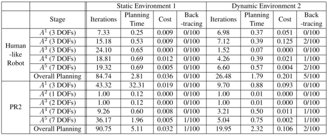
3.1 The performance of our hierarchical planning algorithm is compared with the non-hierarchical ITOMP algorithm. We compute collision-free trajectories in static and dynamic environments. We measure the number of iterations used in the numerical optimization procedure; planning time to find the first collision-free solution; trajectory cost based on Equation (3.1); and the success rate of our planner, i.e., the total number of trials that found a collision-free trajectory. In the static scenes, our hierarchical planner results in up to 14X speedup over the non-hierarchical algorithm. The trajectory costs for the hierarchical and non-hierarchical algorithms are small (less than 0.1), which means the quality of the solution with the hierarchical planner is close to the

trajectory computed by the non-hierarchical planner. . . 41 3.2 We highlight the runtime performance of our planning algorithm in static and

dynamic environments. We show the number of iterations; the planning time to find the first collision-free solution; the trajectory costs; and the number of trials in which back-tracings occur for each stage of our hierarchical planning algorithm, i.e., when a stage fails to find a collision-free trajectory for the corresponding component, the planner merges the component and its parent,

then computes the trajectory of the merged component. . . 42

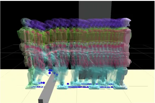
4.1 Planning results for different benchmarks on a single CPU core. We highlight the robot DOFs and the number of potential contact points with the environ-ment. We measure the means and the standard deviations for the number of iterations in the numerical optimization process; the planning time needed to compute the first collision-free solution; and the smoothness of the trajectory for different benchmarks. The smoothness is computed by the sum of joint accelerations at the trajectory waypoints for all active joints, which means that

(12)

4.2 This table compares the feature of our motion planning with dynamic stability algorithm with other approaches. Our approach can handle all the constraints, similar to the direct contact force optimization algorithm (Posa and Tedrake,

2013), but is an order of magnitude faster. . . 58 4.3 Planning results for different benchmarks. We show the number of robots; the

trajectory length that corresponds to the total time that the robots took to reach their goals; the average computation times for the collision avoidance and the

trajectory optimization for each planning step.. . . 59 4.4 Model complexity and the performance of trajectory planning: We highlight

the complexity of each benchmark in terms of number of joints, the number of input discrete poses, and the number of frames that is governed by the length of the motion. We compute the average trajectory planning time per frame for

each benchmark on a multi-core PC. . . 62

5.1 Results obtained from our trajectory computation algorithm based on different levels of parallelization and number of trajectories (for the benchmarks shown

in Fig. 5.8). The planning time decreases when the planner uses more trajectories.. . . 81 6.1 Planning results for our benchmarks. We measure the number of iterations

for the trajectory optimization; planning time; success rate of the planning. We classify the planner as a success if it can find a solution in the maximum iteration limit (2000). As we increase M, the reliability of the planner improves

with respect to various constraints. . . 96 6.2 Planning results for the benchmarks with dynamic obstacles. As we increase

M, the success rate of the planner improves. . . 99

7.1 Performance of our probabilistic collision detection:We measure the

com-putation time of the probabilistic collision detection per single robot configuration.. . . 117 7.2 Planning results in our benchmarks:We measure the planning results of the

computed trajectories: the minimum distance to the human obstacle, trajectory

(13)

LIST OF FIGURES

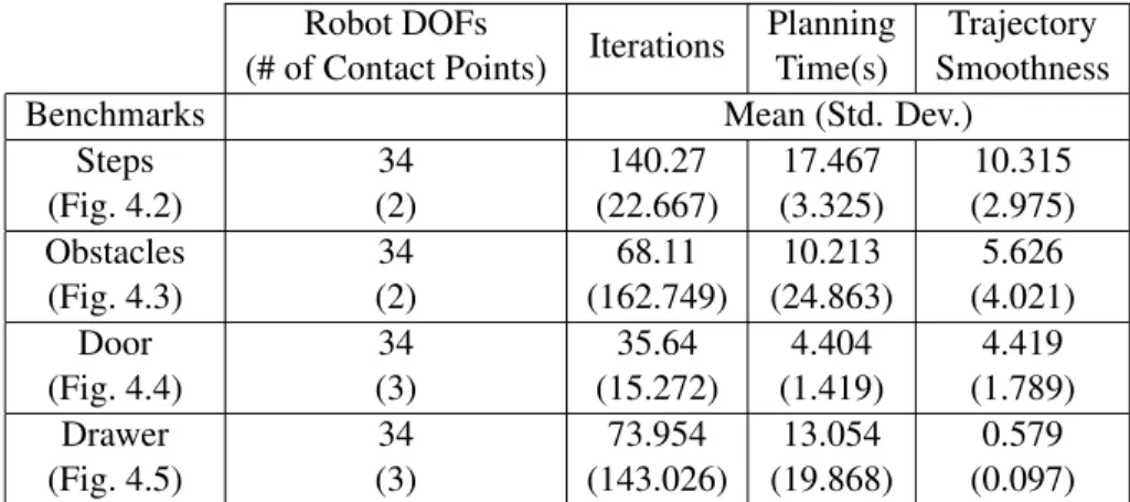
1.1 The task planning repeatedly performs sensing, motion planning and execution

steps in a closed loop. . . 3

2.1 Optimization-based motion planning for dynamic environments. We show how the configuration space changes over time: each plane slice represents the configuration space at timet. In the environment, there are twoC-obstacles: the static obstacleCOs _{and the dynamic obstacle}_COd_{. We need to plan a} trajectory to avoid these obstacles. The trajectory starts at time0, stops at time

T, and is represented by a set of way pointsq1, ...,qk, ...,qN. Supposing that the trajectory is to be executed by the robot during time intervalI = [t0, t1], we only need to consider the conservative boundCOd([t0, t1])for the dynamic obstacle during the time interval. TheC-obstacles shown in the red color

correspond to the obstacles at timet_∈I. . . 21

2.2 The overall pipeline of ITOMP: the scheduling module runs the main algorithm. It gets input from the user and interleaves the planning and execution threads. The Motion Planner module computes the trajectory for the robot and the Robot Controller module is used to execute the trajectory. The planner also

receives updated environment information frequently from sensors. . . 23 2.3 Interleaving of planning and execution. The planner starts at timet0. During

the first planning time budget[t0, t1], it plans a safe trajectory for the first execution interval[t1, t2], which is also the next planning interval. In order to compute the safe trajectory, the planner needs to compute a conservative bound for each moving obstacle during[t1, t2]. The planner is interrupted at timet1 and the ITOMP scheduling module notifies the controller to start execution. Meanwhile, the planner starts the planning computation for the next interval[t2, t3], after updating the bounds on the trajectory of the moving obstacles. Such interleaving of planning and execution is repeated until the robot reaches the goal position. In this example,ninterleaving steps are used,

and the time budget allocated to each step is∆i, which can be fixed or changed adaptively. Notice that if the robot is currently is an open space, the planner

may compute an optimal solution before the time budget runs out (e.g., during[t2, t3]). . . 24 2.4 The planning environment used in experiments related to sensor noise. The

planner computes a trajectory for the right arm of PR2 robot, moving it from the start configuration to the goal configuration while avoiding both static and dynamic obstacles. In the figure, green spheres correspond to static obstacles

(14)

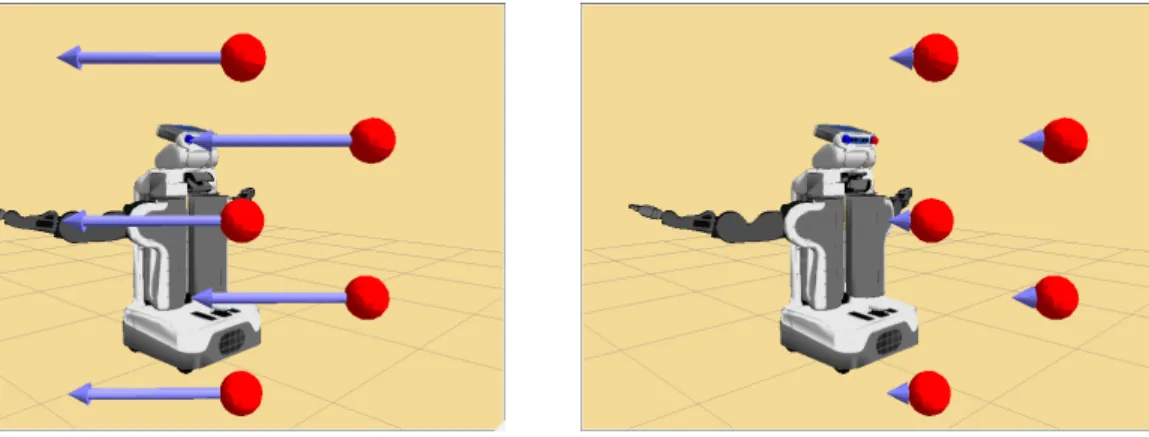
2.5 Planning environments used to evaluate the performance of our planner with moving obstacles with varying speeds. The planner uses the latest obstacle position and velocity to estimate the local trajectory. (a)(b) The obstacles (corresponding to red spheres) in the environment have varying (high or low)

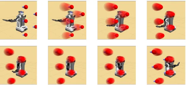
speeds. The size of each arrow corresponds to the magnitude of each’s speed. . . 28 2.6 A collision-free trajectory and conservative bounds of moving obstacles. (a)

There are five moving obstacles. The arrows shows the direction of obstacles. (b)(c) During each step, the planner computes conservative local bounds on obstacle trajectory for the given time step. (b)(c)(d) The robot moves to the goal position while avoiding collisions with the obstacle local trajectory

computed using the bounds. (d) The robot reaches the goal position.. . . 29 2.7 Planning environments used to evaluate the performance of our planner with

different numbers of moving obstacles. . . 30

3.1 An example of hierarchical decomposition for various robots. These hierar-chical decompositions are used to divide a high-dimensional problem into a

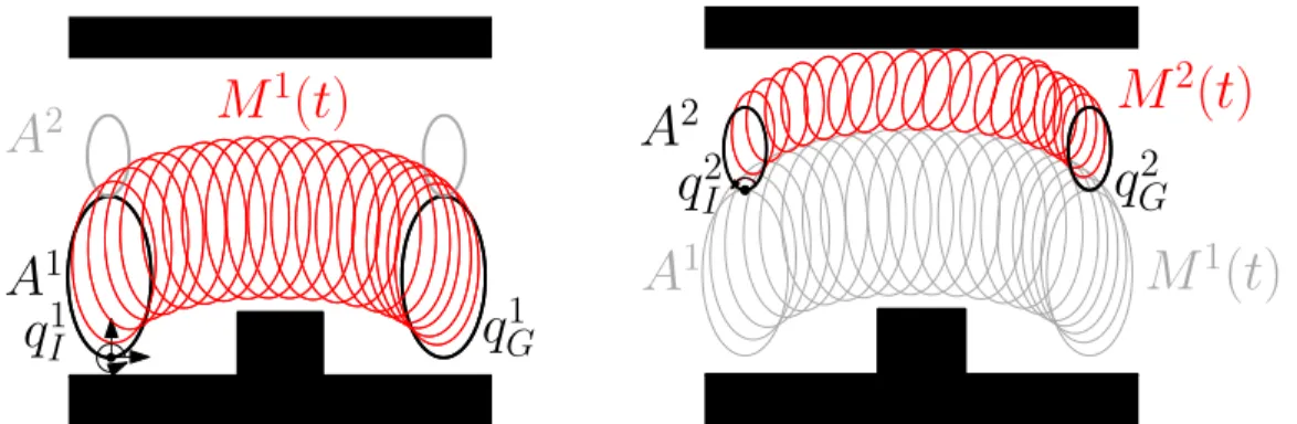
sequence of low-dimensional problems. . . 34 3.2 Incremental trajectory planning. The robot model consists of{A1(3 DOFs),

A2_{(1 DOF)}. (a) During stage}₁_{, the algorithm computes trajectory}_M1₍_t₎_for

A1while avoiding collisions betweenA1 and the obstacle shown in the black

region. (b) During stage2of the planning algorithm, the trajectoryM2(t)for

A2_{is computed while}_A1 _{is assumed to move along the trajectory}_M1₍_t₎_{. . . 36} 3.3 Planning with local refinement. By adjusting the configuration of the jointj1

connectingA1 andA2, we can moveA1 away from the obstacle and leave

more space forA2 _{to pass through. As a result, the planner can compute a}

collision-free solution_M¯2₍_t_{) =}_{_M1₍_t₎_{, M}2₍_t₎_{}. . . 37} 3.4 (a)(b) Hierarchical planning of a PR2 robot and a human-like robot in a static

environment. The planned trajectory for different components is marked using different colors. (c)(d) Planning in dynamic environments. With the static obstacles, we also use human-like obstacles (shown in cyan) that follow a path generated from motion-capture data. The robot does not have anya priori information about the trajectory of this obstacle, which is designed to interrupt

the robot’s trajectory.. . . 43 3.5 Hierarchical planning of HRP-4 robot. Using stability constraints, the

optimization-based planner computes physically plausible walking motion. . . 45

4.1 A humanoid robot makes contactsc1andc2with the ground plane. The gravity wrenchwg and the inertia wrenchwi are applied to the robot. The contact wrenchesw1_candw2_ccan have values in their friction cone. The robot is stable

(15)

4.2 Snapshots of the computed trajectory planned across uneven terrain of varying heights. The proper footstep points are computed during the optimization, and

the entire walking motion trajectory is dynamically stable. . . 56

4.3 Snapshots of the computed trajectory for the environment with obstacles. There is an obstacle between the initial position and the goal position that the robot cannot detour around. The computed trajectory passes over the obstacle. . . 56

4.4 We highlight the smooth and dynamic stable trajectory computed by our planner to perform the specific tasks. The robot uses multiple degrees of freedom, including 14 DOF on the legs to move and 7 DOF on the arm to open the door. . . 56

4.5 We highlight the high-DOF trajectory for the robot to perform the tasks for opening the drawer by our algorithm. . . 57

4.6 Timing breakdown of an iteration of the trajectory optimization. . . 57

4.7 (a)(b)(c)(d) Multi-robot planning benchmarks. (e) Plot of the the planning time of the collision avoidance and the trajectory optimization along the trajectory for a robot. . . 60

4.8 Construction site benchmark scenario. A human-like virtual character navi-gates through various obstacles in 3D space such as scaffolding, metal beams, uneven solid mound etc. . . 63

4.9 A virtual character passes under a scaffold. . . 63

4.10 A virtual character steps over a beam placed on the ground. . . 64

4.11 A virtual character is walking over a uneven solid mound. . . 64

(16)

5.2 The overall architecture of our parallel replanning algorithm. The planner consists of four individual modules (scheduler, motion planner, robot controller, sensor data collection), each of which runs as a separate thread. When the motion planning module receives a planning request from the scheduler, it

launches optimization of multiple trajectories in parallel.. . . 73 5.3 The timeline of interleaving planning and execution in parallel replanning.

In this figure, we assume the number of trajectories computed by parallel optimization algorithm as four. At timet0, the planner starts planning for time interval [t1,t2], during the time budget [t0,t1]. It finds a solution by trying to optimize four trajectories in parallel. At timet1, the planner is interrupted and returns the result corresponding to the best trajectory to scheduler module.

Then the scheduler module executes the trajectory.. . . 74 5.4 The detailed breakdown of GPU trajectory optimization. It starts with the

generation of k initial trajectories. From these initial trajectories, the algo-rithm iterates over stochastic optimization steps. The waypoint costs include collision cost, end effector orientation cost, etc. We also compute joint cost, which might include smoothness costs or the cost of computing the torque constraints. The current trajectory cost is repeatedly improved until the time

budget runs out. . . 75 5.5 The distribution of the distance to the solution in configuration space. The

robot has four revolute joints. We discretize the 4-DOF space and measure the distances to the collision-free space from the trajectories generated from all the discretized points. Environment 1 has 12 small obstacles, and the

environment 2 has 3 obstacles in the scene.. . . 78 5.6 Benefits of a parallel, multi-threaded algorithm in terms of the responsiveness

improvement. We assume that the time costs of different trajectories for optimization are proportional to the distance to the feasible solution. We show the acceleration by varying the number of trajectories on the two distributions

from Fig. 5.5.. . . 79 5.7 Benefits of the parallel algorithm in terms of the performance of the

optimiza-tion algorithm. The graph shows the number of optimizaoptimiza-tion iteraoptimiza-tions that can be performed per second. When multiple trajectories are used on a multi-core CPU (by varying the number of multi-cores), each multi-core is used to compute one single trajectory. The number of iterations performed per second increases as a linear function of the number of cores. In the case of many-core GPU optimization, increasing the number of trajectories results in sharing of GPU resources among different trajectory computations, and the relationship is non-linear. Overall, we see a better utilization of GPU resources if we optimize

(17)

5.8 Planning environment used to evaluate the performance of our planner. The planner computes a trajectory of robot arm which avoids dynamic obstacles and moves horizontally from right to left. Green spheres are static, and red spheres are dynamic obstacles. Figure (a), (b) Show the start and goal

configurations of the right arm of the robot. . . 81 5.9 Parallel replanning in dynamic environments with a human obstacle. The

planner optimizes multiple paths which are smooth and avoid collision with the obstacle. Each colored path corresponds to a different search in the

configuration space. The optimal path for each case is shown in purple.. . . 82 5.10 Success rate and trajectory cost results obtained from the replanning in

dy-namic environments on a multi-core CPU and a many-core GPU. The success rate and trajectory cost is measured for each planner. The use of multiple trajectories in our replanning algorithm results in higher success rates and

trajectories with lower costs and thereby, improved quality.. . . 83 6.1 An overview of our planning algorithm. The roadmap precomputation takes

into account static obstacles and singularity constraints. For a given planning request, M pathsP1, ..., PM are computed using graph search. The

com-puted paths are converted to trajectories, and then refined using trajectory

optimization. . . 89 6.2 (a) Classification of the Configuration space. The obstacle spaceCobsconsists

of disconnected regions, and the near-singular spaceCsingular+ is a region that the distance to the closest singular configuration is smaller than a value.

(b) A roadmap graph built on Fig. 6.2(a) and multiple paths are shown. The nodes and edges on the graph are collision-free and correspond to non-singular configurations. For a path query from an initial configurationQinitto the goal regionqgoal(shown in dark gray region), different non-deformable pathsP1,

P2, andP3are shown in the graph.. . . 90 6.3 Benchmark 1 computes a trajectory for end-effector constraints for X- and

Y-axis rotations. (a) The start (green) and goal (blue) poses are shown. (b) The

computed trajectory is shown. . . 97 6.4 Plots of joint values for the computed trajectory of Benchmark 1. (a) All joint

values in the trajectory are smooth. (b) There are points that the joint values

suddenly change. . . 97 6.5 Benchmark 2 is following a trajectory defined for end-effector positions. (a)

The environment and the constraint trajectory (blue path) are shown. (b) The

computed trajectory is shown. . . 97 6.6 Dynamic environments: (a) We capture the depth map of a scene with a human

arm approaching the arm using a Kinect. (b) 3D octomap is constructed from

(18)

6.7 Demonstration of our constrained planning algorithm in a static environment

with KUKA LBR4+ robot. . . 100

7.1 Approximation of probabilistic collision detection between a sphere obstacle of radiusr2with a probability distributionN(plm,Σlm)and a rigid sphere robot

Bjk(qi)centered atojk(qi)with radiusr1. It is approximated asV ·xmax, whereV is the volume of the sphere with the radius computed as the sum of

two radii,V = 4π₃ (r1+r2)3, andxmaxis the position which has the maximum

probability ofN(plm,Σlm). . . 106 7.2 Comparison of approximated collision probabilities for feasible (P(x)≤

1₋δCL) and infeasible (P(x) >1−δCL) scenarios forδCL = 0.99: We compare the exact collision probability (computed using numerical integra-tion) with approximated probabilities of 1) enlarged bounding volumes (blue contour) (Van den Berg et al., 2012), 2) approximation using object center point (in green) (Du Toit and Burdick, 2011), and 3) our approach that uses the maximum probability point (in red). Our approach guarantees that we do not underestimate the probability, while our approximated probability is close

to the exact probability. . . 109 7.3 Environment belief state estimation for a human obstacle: We

approxi-mate the point cloud from the sensor data using bounding volumes. The shapes of bounding volumes are pre-known in the database, and belief states are defined on the probability distributions of bounding volume poses: (a) input point clouds (blue dots). (b) the bounding volumes (red spheres)with their mean positions (black dots). (c) the probabilistic distribution of mean

positions. 0% confidence level (black) to 100% confidence level (white). . . 110 7.4 Spatial uncertainty:(a) Sphere obstacle and its point cloud samples from a

depth sensor. (b) Probability distribution of a sphere center statepfor a single

point clouddk. (c) Probability distribution ofpfor a partially visible obstacle.

(d) Probability distribution ofpfor a fully visible obstacle. . . 113

7.5 Trajectory Planning: We highlight various components of our algorithm. These include belief space estimation of environment (described in Sec-tion 7.4), probabilistic collision checking (described in SecSec-tion 7.3), and

trajectory optimization. . . 115 7.6 Robot Trajectory with Dynamic Human Obstacles: Static obstacles are

shown in green, the estimated current and future human bounding volumes are shown in blue and red, respectively. Our planner uses the probabilistic collision detection to compute the collision probability between the robot and the uncertain future human motion. (a) When a human is approaching the robot, our planner changes its trajectory to avoid potential future collisions. (b) When a standing human only stretches out an arm, our model-based prediction prevents unnecessary reactive motions, which results in a better robot trajectory

(19)

7.7 Robot trajectory with different confidence and noise levels: Static obsta-cles are shown in green, the estimated current and future human bounding

volumes are shown in blue and red, respectively. . . 120 7.8 Real Robot Experiment:7-DOF Fetch robot arm repeatedly moves between

two points while avoiding collisions with the human. It is noticeable that the robot trajectory deviates more as the human motion becomes faster, in order

to deal with the increased uncertainties in the human motion prediction. . . 121 7.9 Real Robot Experiment:The 7-DOF Fetch robot arm is serving a soda can

on a table, while the robot avoids collisions with the human arm that may

(20)

LIST OF ABBREVIATIONS

CIO Contact-Invariant Optimization

DOF Degree of Freedom

EDT Euclidean Distance Transform

FLOPS FLoating-point Operations Per Second GPU Graphics Processing Unit

ITOMP Incremental Trajectory Optimization for Motion Planning ORCA Optimal Reciprocal Collision Avoidance

PDF Probability Distribution Function

POMDP Partially-Observable Markov Decision Process PRM Probabilistic Roadmap Method

RB-PRM Reachability-Based Probabilistic Roadmap Method ROS Robot Operating System

RRT Rapidly-exploring Random Tree

(21)

CHAPTER 1 Introduction

Physical robots have been used for different applications since the 1960’s. Traditionally, robots were mainly limited to industrial applications such as welding, cutting, or painting. In these cases, robots are operated in confined and static spaces, and they repeat predefined tasks. Given the recent advancements in hardware and sensor technology, robots are increasingly being used in all environments, including homes, malls, restaurants, factories, and outdoor scenes. These environments consist of moving or time-varying obstacles, the motions of which are not known a priori. One driving application is autonomous cars, which are expected to automatically drive in all kinds of conditions and avoid collisions with pedestrians and other vehicles (Katrakazas et al., 2015).

Over the last few decades, high-degree of freedom (DOF) robot systems have been widely used for different applications. These include the use of industrial manipulators for manufacturing and assembly tasks. Most high-DOF robot systems consist of arms or manipulators with redundant DOF, i.e. the system has more than six DOF, which allows the robots to perform dexterous tasks with collision avoidance using their redundancy. In the recent DARPA DRC challenge (Iagnemma and Overholt, 2015), humanoid robots with 30-40 DOF had to perform dexterous tasks such as drilling a hole or rotating a valve. In the future, high-DOF autonomous robot systems are expected to be used for other applications, including: 1) robots for cleaning (not only limited to floors) and cooking/serving in households; 2) entertainment robots that interact with humans in parks and amusement areas; 3) industrial robots that are working next to humans on the factory floors; 4) robots used for search and rescue in disaster areas.

(22)

finding of a feasible robot motion in terms of the given constraints that can be efficiently solved in theconfiguration space(Lozano-Perez, 1983). A robot pose in a 3D workspace is mapped to a point in the configuration space, and the motion planning problem is reduced to a path finding problem in the configuration space. A simple motion planning problem may correspond to the computation of a collision-free path from an initial configuration to the goal configuration. Some tasks such as welding or cutting may have additional Cartesian constraints for the motion planning, i.e. the end effector of the arm will need to follow a certain path in the resulting motion.

There is considerable work on motion planning for high-DOF robots. At a broad level, the previ-ous work can be classified into sampling-based planners and optimization-based planners (LaValle, 2006). Most of the earlier work on practical motion planning algorithms is based on sampling-based algorithms (Kavraki et al., 1996; Kuffner and LaValle, 2000; Jaillet and Sim´eon, 2008; Karaman and Frazzoli, 2011). The key idea in sampling-based approaches is to generate samples in the free configuration space where the robot is collision-free, and connect them with collision-free edges to construct a graph until a collision-free path from the initial configuration to the goal configuration is found. These planners are probabilistically complete (i.e. the probability that they will find a solution approaches one as more samples are added). However, it is relatively difficult to handle many constraints (e.g., trajectory smoothness or dynamic constraints) on the collision-free trajectories computed by sampling-based planners. Non-smooth and jerky paths can cause actuator damages, and balancing constraints are important for humanoid robots.

On the other hand, optimization-based planners pose the motion planning problem in a continuous setting and use optimization techniques to compute the trajectory (Ratliff et al., 2009; Kalakrishnan et al., 2011; Schulman et al., 2014). They generate motion trajectories that can satisfy various constraints simultaneously. Different constraints can be formulated as part of the optimization function for trajectory computation. However, most optimization-based approaches are limited to computing local optimal solutions due to the computational complexities of the global optimization. Furthermore, even the state-of-the-art applications of optimization-based motion planning for high-DOF robots (El Khoury et al., 2013; Lengagne et al., 2013) require a large amount of computation time, which makes them unsuitable for dynamic environments.

(23)

Sense

Plan

Move

Figure 1.1: The task planning repeatedly performs sensing, motion planning and execution steps in a closed loop.

maintenance (for example, evacuation planning for a building or an airplane). Automatically synthesizing plausible motion animations for human-like characters is one of the major challenges in computer graphics in fields such as computer games, virtual reality, and computer animation. This problem of generating dynamically balanced trajectories has also been studied in robotics, and many solutions have been proposed based on optimization-based planning (Mordatch et al., 2012; Al Borno et al., 2013; Wampler et al., 2014) or tree-based search (Bouyarmane and Kheddar, 2011; Escande et al., 2013). However, the complexity and running time of such algorithms can be high, especially as we consider multiple constraints, and resulting motions may not look plausible or are not fast enough for interactive applications.

1.1 Motion Planning in Dynamic Environments

(24)

time interval. Such uncertainty about moving objects makes it hard to plan a safe trajectory for the robot. One solution to overcome this problem is to perform sensing and planning repeatedly (Bowen and Alterovitz, 2014; Sun et al., 2015a). As shown in Fig. 1.1, the robot system works as a closed loop that goes back to the sensing step again to update the environment representation with the latest sensor information after the previously computed planning result is executed.

However, if the planning step takes a long time, it can lead to long delays during the robot’s movement and may cause collisions for robots operating in environments with fast dynamic obstacles. Therefore, instead of computing the complete and optimal plan for the given task, many real-time replanning approaches compute partial or sub-optimal plans for execution that avoid collisions in a limited time step. Different algorithms can be used as the underlying planners in this real-time replanning framework, including sample-based planners (Hauser, 2012; Hsu et al., 2002; Petti and Fraichard, 2005) or search-based methods (Koenig et al., 2003; Likhachev et al., 2005). Most replanning algorithms use fixed time steps (Petti and Fraichard, 2005). Some recent work (Hauser, 2012) computes the timing step in an adaptive manner to balance between safety, responsiveness, and completeness of the overall system.

Control-based approaches (Haschke et al., 2008; Kroger and Wahl, 2010), which can compute trajectories in realtime, are used in many applications that require high responsiveness. They compute the robot trajectory in the Cartesian space, i.e. the workspace of the robot, according to the sensor data. However, the mapping from the Cartesian trajectory to the trajectory in the configuration space of high-DOF robots can be problematic as there can be multiple configurations for a single pose defined in the Cartesian space. Furthermore, control-based approaches tend to compute robot trajectories that are less smooth as compared to the planning approaches that incorporate the estimation of the future obstacle poses. Planning algorithms can compute better robot trajectories in applications in which a good prediction about obstacle motions in a short horizon can be provided.

1.2 Optimization-based Motion Planning

(25)

and it can be refined or smoothed using optimization techniques. The most widely-used method of path optimization is the so-called ‘shortcut’ heuristic, which selects pairs of configurations along a collision-free path and invokes a local planner to replace the intervening sub-path with a shorter one (Chen and Hwang, 1998; Pan et al., 2012). Other approaches are based on elastic bands or elastic strips, which use a combination of mass-spring systems and gradient-based methods to compute minimum-energy paths (Brock and Khatib, 2002; Quinlan and Khatib, 1993).

Other algorithms relax the assumptions about the initial path and may start with an in-collision path. Some recent approaches, such as (Ratliff et al., 2009; Kalakrishnan et al., 2011; Schulman et al., 2014), directly encode the collision-free constraints using a global potential field and compute a collision-free trajectory for robot execution. These methods typically represent various constraints (smoothness, torque, etc.) as soft constraints in terms of additional penalty terms to the objective function. Although these planners do not guarantee planning completeness, they efficiently compute trajectories that optimize over a variety of criteria in many real-world planning scenarios.

In terms of motion planning for high-DOF robots, satisfying dynamic constraints is an important criterion of motion planning. There is considerable work on the maintenance of balance of bipedal robots, which includes techniques based on the inverse pendulum (Kajita and Tani, 1991) or the zero moment point (Huang et al., 2001). However, these approaches are limited to planar ground (i.e. flat surfaces). Recently, many optimization-based approaches have integrated stability constraints directly into trajectory optimization (Lee et al., 2005; Lengagne et al., 2010; Schultz and Mombaur, 2010). Mordatch et al. (2012) use a contact-invariant optimization formulation, along with a simplified physics model, to generate various motions for animated characters. Posa et al. (2013) directly optimize the contact forces along with the state of the robot and the user input.

(26)

1.3 Motion Planning of High-DOF Robots

One of the main challenges in terms of planning in dynamic environments is that the planning algorithm must be responsive to unpredictable situations, which requires realtime planning capability in terms of computing or updating the trajectory. Due to the rapid advances in multi-core and many-core commodity processors, designing efficient parallel planning algorithms that can benefit from their computational capabilities is an important topic in robotics. Many parallel algorithms have been proposed for motion planning by utilizing the properties of configuration space (Lozano-Pérez and O’Donnell, 1991) that exploit distributed clusters, shared-memory systems, or commodity parallel processors. Distributed clusters have been widely used for solving compute-intensive problems. Clusters are defined as a large number of connected machines or nodes, each of which has local memory. A big computational problem is divided into small pieces and assigned to different processors in the cluster for parallel computation. Many parallel techniques have been proposed to improve the performance of planning using distributed clusters. Pérez and O’Donnell (1991) compute the primitive map of a 3D configuration space using parallel computation. Amato et al. (1999) propose a parallel PRM planning approach that has scalable speedups. Jacobs et al. (2012) propose an algorithm based on subdividing the configuration space (Brooks and Lozano-Pérez, 1985) and use clusters to expand the tree in a different region of the configuration space. Some approaches combine PRM and RRT in order to use the massive parallelism (Plaku and Kavraki, 2005). Nowadays, commodity processors in a single machine have multiple cores. Although these systems have fewer cores and less overall processing power than large distributed clusters, multiple threads running on such shared-memory processors have access to the same memory and there is no major overhead of transferring the data between the nodes in a cluster. Many parallel RRT algorithms have been proposed for shared-memory systems (Carpin and Pagello, 2002; Aguinaga et al., 2008). Parallel algorithms on shared-memory systems have better efficiency than clusters because the multiple threads can share the same tree data structure on shared memory (Sucan and Kavraki, 2012). Updates of the shared tree require synchronization, and the performance can be improved using lock-free data structures (Ichnowski and Alterovitz, 2014).

(27)

2000). Recently, the general purpose GPU technology allows efficient use of the GPUs using appropriate interfaces (e.g., CUDA, OpenCL). g-Planner (Pan et al., 2010a) uses many-core GPU processors to parallelize and accelerate PRM approach. Kider et al. (2010) propose a GPU-based R* algorithm for 6-DOF problems. Bialkowski et al. (2011) use multiple cores on GPUs to perform parallel collision checking along different edges of RRT.

For the planning of high-DOF robots, hierarchical approaches have been used to decompose a higher-dimensional planning problem into several lower-dimensional planning problems. This divide-and-conquer method can substantially reduce the complexity of the planning problem (Brock and Kavraki, 2001), and the incompleteness of the resulting planning algorithms can be improved by greedy techniques based on back-tracing (Alami et al., 1995). Hierarchical methods have been used to improve performance for articulated robots (Brock and Kavraki, 2001) or for multi-robot systems (Isto and Saha, 2006). Different coordination schemes (Erdmann and Lozano-P´erez, 1986; Saha and Isto, 2008) have been proposed to guarantee that the decomposed planner finds solutions for the robots’ whole bodies. Simple decomposition into lower- and upper-body has been used to plan the motion for human-like robots (Arechavaleta et al., 2004); a more detailed decomposition has been used to accelerate whole-body planning for high-DOF robots using sampling-based planners (Zhang et al., 2009; Pan et al., 2010b). Recently, hierarchical mechanisms have also been used to accelerate the Markov Decision Process (Barry et al., 2011) and task planning (Kaelbling and Lozano-P´erez, 2011a,b).

1.4 Modeling Uncertainties in Dynamic Environments

(28)

problems that are high-dimensional. Therefore, many efficient approximations (Silver and Veness, 2010; Kurniawati and Yadav, 2013; Somani et al., 2013) and parallel techniques (Shani, 2010; Lee and Kim, 2013) have been proposed to provide a better estimation of the belief space. Most approaches for continuous state spaces use Gaussian belief spaces, which are estimated using Bayesian filters (e.g., Kalman filters) (Leung et al., 2006; Platt Jr et al., 2010). Algorithms using Gaussian belief spaces have also been proposed for the motion planning of high-DOF robots (Van den Berg et al., 2012; Sun et al., 2015b), but they do not account for environment uncertainty or imperfect obstacle information. Instead, most planning algorithms handling environment uncertainty deal with issues arising from visual occlusions from the cameras (Missiuro and Roy, 2006; Guibas et al., 2010; Kahn et al., 2015; Charrow et al., 2015). In terms of dynamic environments, motion planning with uncertainty algorithms is mainly limited to simple robot shapes (Du Toit and Burdick, 2012; Bai et al., 2015), where the robots are modeled as circles, or to specialized applications such as people tracking (Bandyopadhyay et al., 2009).

(29)

the object for a given standard deviation. This may correspond to an ellipsoid (Bry and Roy, 2011) or a sigma hull (Lee et al., 2013). These approaches provide an upper bound for the given confidence level. However, the computed volume overestimates the probability and can be much bigger than the actual volume corresponding to the confidence level, which can cause failure to find existing feasible trajectories in motion planning. Many other approaches have been proposed to perform probabilistic collision detection on point cloud data. Bae et al. (2009) presented a closed-form expression for the positional uncertainty of point clouds. Pan et al. (2011) reformulate the probabilistic collision detection problem as a classification problem and compute per point collision probability. However, these approaches assume that the environment is static. Other techniques are based on broad phase data structures that handle large point clouds for realtime collision detection (Pan et al., 2013).

1.5 Thesis Statement

Motion planning of high-DOF robots in dynamic and uncertain environments can be formulated as a trajectory optimization problem, and the performance and reliability of the planning can be improved using incremental optimization, parallel computation, and efficient cost approximation.

1.6 Main Results

(30)

1.6.1 Incremental Trajectory Optimization

In order to deal with unpredictable dynamic environments, we present a novel optimization-based motion planning algorithm using replanning, which interleaves planning with execution. We compute a conservative local bound on the trajectory of each obstacle over a short time and use the bound to compute a collision-free trajectory for the robot using the geometric collision detection. We model the collision constraint between the robot and moving obstacles as a cost function, and stochastically optimize the trajectory with the trajectory smoothness cost. The trajectory is repeatedly updated while it is executed in order to minimize the error between the estimation and the actual trajectory of the moving obstacles. Our approach efficiently computes collision-free and also smooth trajectories.

We also provide a cost function corresponding to various task constraints for high-DOF robots that are integrated into our optimization formulation. We demonstrate how our motion planning approach can efficiently compute trajectories for various applications including Cartesian planning of industrial manipulators, humanoid robot planning with dynamic stability constraints, high-DOF multi-agent simulation, and virtual human motion synthesis in crowded scenes.

1.6.2 Efficient Motion Planning of High-DOF Robots

(31)

Second, we propose a roadmap precomputation approach to compute initial trajectories of multiple trajectory optimization. We precompute a sparse roadmap using visibility tests, that takes into account static obstacles in the environment as well as singular configurations. At runtime, multiple non-redundant paths in the roadmap are used as initial trajectories for the runtime trajectory optimization. The precomputation improves the multiple trajectory optimization in complex static environments with dynamic obstacles.

Third, we present a novel hierarchical planning algorithm for high-DOF robots. The high-DOF robot is treated as a tightly coupled system, and we incrementally use constrained coordination to plan its motion. We decomposes the high-dimensional motion planning problem into a sequence of low-dimensional sub-problems. Then we compute feasible trajectories using optimization-based planning and trajectory perturbation for each sub-problem. The resulting algorithm computes feasible trajectories of 20-40 DOF robots in almost real-time.

1.6.3 Efficient Approximation of Environment Uncertainties

In order to deal with the uncertainties of obstacle motions in dynamic environments, we first present a novel approach to perform probabilistic collision detection between a robot and imperfect obstacle representations in dynamic environments. Next, we present a prediction algorithm for obstacle motion using a motion model that accounts for both spatial and temporal uncertainties. We model these uncertainties using Gaussian distributions and use the Kalman filter to predict the future obstacle motions. We present an efficient algorithm for approximating the collision probability between the robot and the predicted future obstacle positions. Our approach computes more accurate probabilities as compared to prior approaches that perform exact collision checking with enlarged obstacle shapes. Moreover, we can guarantee that our computed probability is an upper bound on the actual collision probability.

(32)

1.7 Organization

The rest of this thesis is organized as follows.

Chapter 2presents a motion planning algorithm for dynamic environments using trajectory optimization. We describe how our approach incrementally improves the robot trajectory using trajectory optimization in a replanning framework. We provide the formulation of the obstacle cost in the optimization which is used to avoid collision between the robot and dynamic obstacles in the environment. We demonstrate the performance of our approach using 7-DOF PR-2 robot in a simulated environment with moving obstacles.

Chapter 3describes the hierarchical planning framework for high-DOF robots. We present our multi-stage trajectory optimization algorithm based on hierarchical decomposition, and describe our decomposition scheme and trajectory optimization approach for sub-problems using the constrained coordination and the local refinement. We validate our hierarchical planning algorithm with 20- and 34-DOF robots in environments with moving obstacles.

Chapter 4presents how to model constraints of high-DOF robots in trajectory optimization. We provide the formulation of the stability and contact constraints in the trajectory optimization, and describe our strategy for the efficient optimization. We demonstrate the performance of our high-DOF robot planning approach, and applications that extend our approach to the multi-agent simulation and virtual human motion synthesis scenarios.

Chapter 5presents a GPU-based parallel multi-trajectory optimization. We describe how our parallel algorithm is efficiently mapped to GPUs in order to utilize their parallel capabilities. We prove that our multiple trajectory optimization approach accelerates the planning and improves the probability to find a feasible solution, and analyze the improvements in environments with different complexities. We demonstrate the real-time performance of our approach in a simulated environment with human-like obstacles.

(33)

our approach using a 7-DOF KUKA robot arm in environments with moving obstacles captured using depth sensors.

Chapter 7describes our probabilistic collision detection algorithm for high-DOF robots under environment uncertainties. We present a prediction algorithm for human obstacles using Kalman filters. We provide the formulation of the collision probability approximation which is efficient and provides an upper bound on the actual collision probability. We present a motion planning algorithm for high-DOF robots based on our probabilistic collision detection. We highlight our approach computes efficient and reliable trajectories in simulated environments as well as with a 7-DOF Fetch robot arm in real-time.

(34)

CHAPTER 2

Incremental Trajectory Optimization

2.1 Introduction

Planning collision-free motion in a dynamic environment is an important problem in many robotics applications, including autonomous navigation and task planning. There has been extensive literature on motion planning and navigation of robots in dynamic environments (Fiorini and Shiller, 1998; Chakravarthy and Ghose, 1998). However, practical use of high-DOF robots has been limited to static environments due to the high computational complexity.

Some recent work use replanning framework with random sampling-based planning (Kavraki et al., 1996; Kuffner and LaValle, 2000) to efficiently compute partial or sub-optimal plans to avoid delays in its handling of moving obstacles (Petti and Fraichard, 2005; Bekris and Kavraki, 2007; Hauser, 2012). However, these sampling-based approaches tend to compute non-smooth jerky motions, and it is difficult to incorporate dynamic constraints which can be required for high-DOF robots.

2.1.1 Main Results

(35)

robot respond quickly to the dynamic environments, we interleave planning with task execution: that is, instead of solving the optimization problem completely, we assign a time budget for planning and interrupt the optimization solver when the time runs out. The computed trajectory may be sub-optimal, which means that 1) its objective cost may not be minimized; 2) the collision-free constraints or other additional constraints may not be completely satisfied. The robot then executes over the short time interval based on this sub-optimal path computation. We repeat these steps until the robot reaches the goal position. During each iterative step, we update the conservative bound on the object’s position and also account for any new objects that may have entered the robot’s workspace. The updated environment information is incorporated into the optimization formulation, which uses the sub-optimal result from the last step as the initial solution and tries to improve it incrementally within the given timing budget. We demonstrate the performance of our replanning algorithm in the ROS simulation environment where the PR2 robot tries to perform manipulation task with its 7-DOF robot arm.

2.1.2 Organization

The rest of this chapter is organized as follows. We survey related work on planning for dynamic environments and replanning in Section 2.2. Section 2.3 introduces the notation used in the chapter and gives an overview of our approach. We present our optimization-based replanning algorithm (ITOMP) in Section 2.4. We highlight its performance on simulated dynamic environments in Section 2.5. We direct the readers to the project webpage (http://gamma.cs.unc.edu/ ITOMP/) for the videos as well as the related publication (Park et al., 2012).

2.2 Related Work

In this section, we give a brief overview of prior work on motion planning in dynamic environ-ments, realtime replanning and optimization-based planning.

2.2.1 Planning in Dynamic Environments

(36)

a short horizon and set a high cost around the obstacles (Likhachev and Ferguson, 2009). Another common approach is to use velocity obstacles, which are used to compute appropriate velocities to avoid collisions with dynamic obstacles (Fiorini and Shiller, 1998; Wilkie et al., 2009). However, these methods cannot give any guarantees on the optimality of the resulting trajectory.

Some of the planning methods handle the continuous state space directly, e.g., RRT variants have been proposed for planning in dynamic environments (Petti and Fraichard, 2005). For discrete state spaces, efficient planning algorithms for dynamic environment include variants of A* algorithm, which are based on classic heuristic searches (Phillips and Likhachev, 2011b,a) and roadmap-based algorithms (van den Berg and Overmars, 2005).

Most planning algorithms for dynamic environments (van den Berg and Overmars, 2005; Phillips and Likhachev, 2011b) assume that the inertial constraints, such as acceleration and torque limit, are negligible for the robot. Such an assumption implies that the robot can stop and accelerate instantaneously, which may not be the case for a physical robot.

2.2.2 Real-time Replanning

(37)

2.2.3 Optimization-based Planning Algorithms

Optimization techniques can be used to compute a robot trajectory that is optimal under some specific metrics (e.g., smoothness or length) and that also satisfies various constraints (e.g., collision-free and dynamics constraints). Some algorithms assume that a collision-collision-free trajectory is given and it can be refined or smoothened using optimization techniques. These include ’shortcut’ heuristic (Chen and Hwang, 1998), elastic bands or elastic strips planning (Brock and Khatib, 2002; Quinlan and Khatib, 1993). Other algorithms relax the assumptions about the initial path and may start with an in-collision path. Some recent approaches, such as (Ratliff et al., 2009; Kalakrishnan et al., 2011), directly encode the collision-free constraints using a global potential field and compute a collision-free trajectory for robot execution. These methods typically represent various constraints (smoothness, torque, etc.) as soft constraints in terms of additional penalty terms to the objective function.

2.3 Overview

In this section, we introduce the notation used in the rest of the chapter and give an overview of our approach.

We use the symbolCto represent the configuration space of a robot, including severalC-obstacles and the free spaceCf ree. Let the dimension ofCbeD. Each element in the configuration space, i.e.,

a configuration, is represented as a dim-Dvectorq.

For a single planning step, suppose there areNsstatic obstacles andNddynamic obstacles in the environment. The number of dynamic obstacles is changed between the steps as the sensor introduces new obstacles and removes out of range obstacles and the information is kept for a planning interval. We assume that these obstacles are all rigid bodies. For static obstacles, we denote them asOsj,j= 1, ..., Ns. For dynamic obstacles, as their positions vary with time, we denote them asOd

j(t),j= 1, ..., Nd.OjsandOdj(t)correspond to the objects in the workspace, and we denote their correspondingC-obstacles in the configuration space asCOs

j andCOdj(t), respectively. In the ideal case, we assume that we have complete knowledge about the motion and trajectory of dynamic obstacles, i.e., we know the functionsOd

(38)

Moreover, the recent position and velocity of obstacles computed from the sensors may not be accurate due to the sensing error. In order to guarantee safety of the planning trajectory, we compute a conservative local bound on the trajectories of dynamic obstacles during planning. Given the time instancetcur, the conservative bound for the moving objectOd

j at timet > tcurbounds the shape corresponding toOd

j(t), and is computed as:

Od_j(t) =c(1 +es·t)Ojd(t) (2.1) whereesis the maximum allowed sensing error. As the sensing error increases the conservative bound becomes larger. When an obstacle has a constant velocity, it is guaranteed that the conservative bound includes the obstacle during the time period corresponding tot > tcurwithc= 1. However, if an obstacle changes its velocity, we have to use a larger value of c in our conservative bound, and it would be valid for a shorter time interval. We can define the conservative bound for a moving object Od

j during a given time intervalI = [t0, t1]as follows:

Odj(I) = [

t∈I

Odj(t),∀t∈I, t > tcur. (2.2)

Similarly, we can define conservative bounds in the configuration space, which are denoted asCOd_j(t) andCOd_j(I), respectively.

We treat motion planning in dynamic environments as an optimization problem in the con-figuration space, i.e., we search for a smooth trajectory that minimizes the cost corresponding to collisions with moving objects and some additional constraints, such as joint limit or acceleration limit. Specifically, we consider trajectories corresponding to a fixed time durationT, discretized into N waypoints equally spaced in time. In other words, the discretized trajectory is composed ofN

configurationsq1, ...,qN, whereqiis a trajectory waypoint at time _Ni−−11T. We can also represent the trajectory as a vectorQ∈ RD·N_:

Q= [qT₁,q₂T, ...,qT_N]T. (2.3)

(39)

Similarly to previous work (Ratliff et al., 2009; Kalakrishnan et al., 2011), our optimization problem is formalized as:

min

q1,...,qN

N X

i=1

c(qi) + 1 2kAQk

2_, _(2.4)

wherec(_·)is an arbitrary state-dependent cost function, which can include obstacle costs for static and dynamic objects, and additional constraints such as joint limit and torque limit. That is, the cost function can be divided into three parts:

c(q) =cs(q) +cd(q) +co(q), (2.5)

wherecs(·)is the obstacle cost for static objects,cd(·)is the obstacle cost for moving objects and

co(·)is the cost for additional constraints. Ascd(·)changes along with time due to movement of dynamic obstacles, we sometimes denote it asct_d(·)to show the dependency on time explicitly.Ais

a matrix that is used to represent the smoothness costs. We chooseAsuch that_kAQ_k2represents

the sum of squared accelerations along the trajectory. Specifically,Ais of the form

A=                   

1 0 0 0 0 0

−2 1 0 · · · 0 0 0

1 −2 1 0 0 0

... ... ...

0 0 0 1 −2 1

0 0 0 _{· · ·} 0 1 ₋2

0 0 0 0 0 1

                  

⊗ID×D, (2.6)

where⊗denotes the Kronecker tensor product andID×D is a square matrix of sizeD. It follows that_Q¨ ₌_AQ_{, where}_Q¨ _{represents the second order derivative of the trajectory}_Q_.

The solution to the optimization problem in Equation (2.4) corresponds to the optimal trajectory for the robot:

Q∗ =_{q∗₁ =qs,q∗2, ...,q∗N−1,q∗N =qg}. (2.7) However, notice thatQ∗is guaranteed to be collision-free with dynamic obstacles only during

(40)

motion of the moving objects, rather than an exact model of the moving objects’ motion, the cost functionct_d(_·)is only valid within a short time interval. In order to associate a period of validity with the result of our optimization algorithm, we useQ∗_Ito represent the planning result that is valid

during the intervalI = [t0, t1]⊆[0, T].

In order to improve robot’s responsiveness and safety, we interleave planning and execution threads, in which the robot executes a partial or suboptimal trajectory (based on a high-rate feedback controller) that is intermittently updated by the replanning thread (at a lower rate) without interrupting the execution. We assign a time budget∆kto thek-th step of replanning, which is also the maximum allowed time for execution of the planning result from last step. We use a constant timing budget ∆t= ∆, but our approach can be easily extended to use a dynamic timing budget that is adaptive to replanning performance (Hauser, 2012). The interleaving strategy is subject to the constraint that the current trajectory being executed cannot be modified. Therefore, if the replanning result is sent to the robot for execution at timet, it is allowed to run for time∆, and no portion of the

computed trajectory beforet+ ∆may be modified. In other words, the planner should start planning from t+ ∆. Due to limited time budget, the planner may not be able to compute an optimal

solution of the optimization function shown in Equation (2.4) and the resulting trajectory may be, and usually is, sub-optimal. Its cost may be greater than or equal to the cost of the optimal trajectory

Q∗. i.e.,f(Q∗_I) _≤ f(Q∗_I), where we denote the resulting trajectory from the planner asQ∗_I, and f(Q) =PN

i=1c(qi) +1₂kAQk2.

2.4 ITOMP : Incremental Trajectory Optimization for Motion Planning in Dynamic Envi-ronments

(41)

dynamic obstacleCOd

static obstacle_COs

q

₁

q

_k

q

_N

0 t

T

C-Space at different time

I= [t0, t

1]

COd([t0, t1])

Figure 2.1: Optimization-based motion planning for dynamic environments. We show how the configuration space changes over time: each plane slice represents the configuration space at timet.

(42)

2.4.1 Obstacle Costs

Similarly to prior work (Kalakrishnan et al., 2011; Ratliff et al., 2009), we model the cost of static obstacles using signed Euclidean Distance Transform (EDT). We start with a boolean voxel representation of the static environment, obtained either from a laser scanner or from a triangle mesh model. Next, the signed EDTd(x)for a 3D pointxis computed throughout the voxel map. This

provides information about the distance fromxto the boundary of the closest static obstacle, which

is negative, zero or positive whenxis inside, on the boundary or outside the obstacles, respectively.

One advantage of EDT is that it can encode the discretized information about penetration depth, contact and proximity in a uniform manner and can make the optimization algorithm more robust. After the signed EDT is computed, the planning algorithm can efficiently check for collisions by table lookup in the voxel map. In order to compute the obstacle cost, we approximate the robot shape Bby a set of overlapping spheresb∈ B. The static obstacle cost is as follows:

cs(qi) = X

b∈B

max(+rb−d(xb),0)kx˙bk, (2.8)

whererb is the radius of one sphereb,xbis the 3D point of spherebcomputed from the kinematic model of the robot in configurationqi, andis a small safety margin between robot and the obstacles.

The speed of sphereb,kx˙bk, is multiplied to penalize the robot when it tries to traverse a high-cost region quickly. The static obstacle cost is zero when all the sphere are at leastdistance away from the closest obstacle.

EDT computation is efficient for static obstacles but cannot be applied to dynamic obstacles, though a GPU-based parallel EDT computation algorithm could be used (Sud et al., 2004). The reason is that the movement of dynamic obstacles implies that EDT needs to be recomputed during each time step and it is hard to perform such computation in real-time on current CPUs. Instead, we perform geometric collision detection between the robot and moving obstacles and use the collision result to formalize the dynamic obstacle cost. Given a configurationqi on the trajectory and the geometric representation of moving obstaclesOs

(43)

Ready

Monitor

Finish

Goal

Motion Planner

Robot Controller

Sensor

Setting

Scheduling Module

Data

Figure 2.2: The overall pipeline of ITOMP: the scheduling module runs the main algorithm. It gets input from the user and interleaves the planning and execution threads. The Motion Planner module computes the trajectory for the robot and the Robot Controller module is used to execute the trajectory. The planner also receives updated environment information frequently from sensors.

cost corresponding to configurationqiis given as:

cd(qi) = X

j

is collide(Osj(

i−1

N −1T),B), (2.9)

whereis collide(·,·)returns one when there is a collision and zero otherwise. Theis collide

function can be performed efficiently using object-space collision detection algorithms, such as (Gottschalk et al., 1996). This obstacle cost function is only used during a short or local time interval, i.e. from replanning’s start timetto its end timet+ ∆, since the predicted positions of

dynamic obstacles can have high uncertainty during a long time horizon.

2.4.2 Dynamic Environment and Replanning

(44)

PLANNING PLANNING PLANNING PLANNING

EXECUTION

EXEC.

EXECUTION EXECUTION

step0 step1 step2 stepn−1 stepn

t0 t1 t2 t3 tn−1 tn tn+1

∆0 ∆1 ∆2 ∆n−1 ∆n tf

goal

time

predict model in[t1, t2] predict model in[t2, t3] predict model in[t3, t4] predict model in[tn,∞]

Figure 2.3: Interleaving of planning and execution. The planner starts at timet0. During the first planning time budget[t0, t1], it plans a safe trajectory for the first execution interval[t1, t2], which is also the next planning interval. In order to compute the safe trajectory, the planner needs to compute a conservative bound for each moving obstacle during[t1, t2]. The planner is interrupted at time

t1 and the ITOMP scheduling module notifies the controller to start execution. Meanwhile, the planner starts the planning computation for the next interval[t2, t3], after updating the bounds on the trajectory of the moving obstacles. Such interleaving of planning and execution is repeated until the robot reaches the goal position. In this example,ninterleaving steps are used, and the time budget

allocated to each step is∆i, which can be fixed or changed adaptively. Notice that if the robot is currently is an open space, the planner may compute an optimal solution before the time budget runs out (e.g., during[t2, t3]).

the environment frequently and the planner needs to be interrupted to update the description of the environment.

In order to handle uncertainty from moving obstacles and provide high responsiveness, ITOMP interleaves planning and execution of the robot. As illustrated in Figure 2.2, ITOMP consists of several parts: the scheduling module, the motion planner, the robot controller and the data-collecting sensor. The scheduling module gets the goal information as input and controls the other modules. When a new goal position is set, the scheduling module sends a new trajectory computation request to the motion planner. When the motion planner computes a new trajectory that is safe within a short horizon, the scheduling module notifies the robot controller to execute the trajectory. Meanwhile, it also sends a new request to the motion planner to compute a safe trajectory for the next execution interval. The planner also needs to incorporate the updated environment description from the sensor data. Since the motion planner runs in a separate thread, the scheduling module does not need to wait for the planner to terminate. Instead, it checks whether the robot reaches the goal, updates the dynamic environment description, and checks whether the planner has computed a new trajectory.

The details about the interleaved planning and execution method are shown in Figure 2.3. The

(45)

budget for the current step of execution. During thei-th time step, the planner tries to generate a

trajectory by solving the optimization problem in Equation 2.4. The trajectory should be valid during the next step of execution, i.e., during the time interval[ti+1, ti+2].

Due to the limited time budget, the planner may only be able to compute a sub-optimal solution before it is interrupted. The sub-optimal solution may not be collision-free or may violate some other constraints during the next execution interval[ti+1, ti+2]. To handle such cases, we use two techniques. First, we assign higher weights to the obstacle costs related to the trajectory waypoints during the interval[ti+1, ti+2], which biases the optimization solver to reduce the cost during the execution interval. If the optimization result is not valid during the execution interval, ITOMP’s scheduling module chooses not to execute during the following execution interval. This approach keeps the planner from violating hard constraints(e.g. torque, end effector orientation, etc.) and allocates more time to the planner to improve the result. If the optimization result is valid but not optimal, i.e., the cost is not minimized during time interval[ti+2,∞], the planner can also improve it incrementally during following time intervals. The time budget for each step of short-horizon planning can be changed adaptively according to the quality of the resulting trajectory, which tries to balance the robot’s responsiveness and safety (Hauser, 2012).

Notice that usually the optimization can converge to local optima quickly because during the

i-th step planning we use the result of(i₋1)-th step as the initial value. On the other hand, the

optimization algorithm tends to compute a sub-optimal solution when the robot is near a region with multiple minima in the configuration space or a narrow passage.

2.5 Results