Weizi Li, Dong Nie, David Wilkie,
and Ming C. Lin, Fellow, IEEE
The Department of Computer Science,
University of North Carolina at Chapel Hill,
Chapel Hill, NC, 27599 USA
E-mail: weizili,dongnie,wilkie,[email protected]
Citywide Estimation
of Traffic Dynamics
via Sparse GPS Traces
Digital Object Identifier 10.1109/MITS.2017.2709804 Date of publication: 25 July 2017
I. Introduction
T
raffic is ubiquitous in modern cities, and it im-pacts the social, economic, and environmental development of the world. Ever-present grid-lock and congestion challenge transportation researchers and urban planners. According to the 2015 Urban Mobility Scorecard [2], traffic congestion causes an extra 6.9 billion travel hours and 3.1 bil-lion gallons of fuel consumption in a year. The con-gestion costs are approximately $160 billion in the United States, more than £13 billions in the United Kingdom, and over one trillion dollars worldwide.Abstract—Traffic congestion is a perpetual challenge
As more and more metropolitan areas around the world experience increasingly severe traffic conditions, the ability to analyze and understand traffic dynamics is becoming ever more crucial.
Traditionally, measurements of traffic states are collect-ed through dcollect-edicatcollect-ed sensors such as loop detectors and video cameras [3]. While these sensors produce relatively accu-rate measurements, the high expenditures for installation
and maintenance prevent them from being deployed over a large network and cause them to be used in limited loca-tions on major roads and highways. Consequently, the lack of sensing infrastructure for arterial streets—which comprise the majority of a city—has made the traffic monitoring task substantially more difficult.
So far, dispersed probe vehicle reports (i.e., GPS traces) are the most promising data source in estimating citywide traffic dynamics. However, such data are of limited useful-ness for two reasons: first, inevitable errors in measure-ment and transmission often yield reported locations off
the road; second, due to energy and privacy concerns, GPS data commonly have a low sampling rate, meaning that the time gap between consecutive reports is large (e.g., 230s), and a low penetration rate, meaning only a small portion of the traffic population is participated in sending reports.
Together these features introduce a large degree of un-certainty to the data. In order to accurately infer traffic dy-namics from such noisy measurements, several steps are required. First, off-the-road GPS points need to be mapped onto the road network, and the probes’ true traversed paths need to be identified. This process is called map-matching. Second, the time taken to travel each road segment must be accurately estimated. Because of the low sampling rate, the identified path between two nearby GPS points is likely to cover multiple road segments, and only the aggregate travel time (i.e., the difference between GPS timestamps) is known. Consequently, the aggregate travel time needs to be decomposed and distributed to individual road segments. These operations are performed in travel time allocation. Third, in order to understand the full traffic dynamics of a road network, traffic data are needed over longer peri-ods of time for each road segment. However, GPS data often do not provide complete temporal coverage for a road seg-ment. In particular, they are scarce in the late night and early morning hours. Currently, the missing information is filled in through missing value completion.
Many efforts have been made towards alleviating the aforementioned problems over the recent years. To be spe-cific, in reference to map-matching, the data’s low sampling rate introduces problems; two consecutive reports are likely to be spatially far apart, and there may be many paths con-necting the two reports in a complex urban environment, making the identification of the true traversed path difficult. To alleviate this issue, many approaches have been proposed that use the shortest-distance criterion [1], [4]–[8]. While the shortest-distance assumption is viable when a road network is under or close to the free-flow condition, this assumption induces bias in a congested environment, where other paths can be traveled in a shorter time than the shortest-distance path. Once introduced, this bias will be carried over to the subsequent step (i.e., travel time allocation), deteriorating the estimation accuracy.
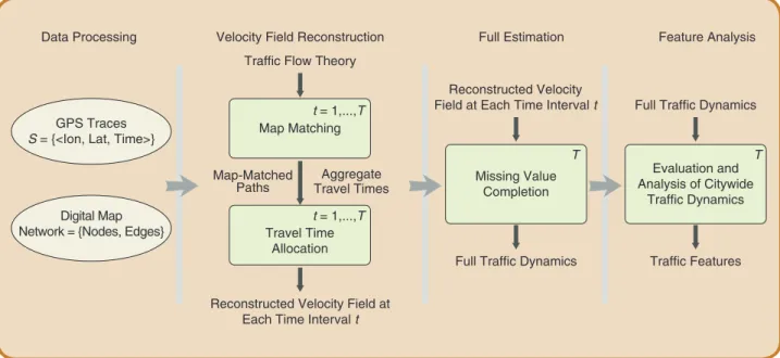
matching. Along with a travel-time allocation technique adapted from [11], a novel computation scheme is designed to reconstruct the velocity field of a road network. In the second phase, exploiting the sparsity embedded in traffic patterns, we have developed a novel method based on the Compressed Sensing [12], [13] algorithm to fill in missing travel information over an entire traffic period. The over-view of our framework pipeline is shown in Figure 1.
The effectiveness of our approach has been extensively evaluated and compared to a state-of-the-art method, using a synthetic road network and traffic data from the city of San Francisco. The results demonstrate major improvements over existing methods in various steps during the estima-tion process. In summary, our contribuestima-tions include:
■ A novel perspective in addressing map-matching of
sparse GPS traces and an improved travel time allo-cation technique that incorporates estimated traf-fic conditions;
■ An efficient method for estimating missing travel
in-formation by exploring sparse structures embedded in traffic patterns;
■ Extensive analysis of our method’s
performance and comparison of our method to existing methods under various traffic scenarios. The rest of paper is organized as follows. In Section II, we discuss related work and highlight the differences between our work and existing studies. In Section III, we take a holistic view of map matching and travel time alloca-tion problems, and detail the process of reconstructing the velocity field of a road network. In Section IV, we explain our method on estimating missing travel information; In Section V, we show estimated traffic dynamics of San Francisco and analyze key features within the recovered traffic pattern. We conclude with a discussion of future work in Section VI.
II. Related Work
Over the last few decades, the estimation of traffic condi-tions has gained increasing scholarly attention [14]–[19]. Early works on traffic estimation have studied traffic states on highways using relatively accurate measurements from stationary sensors such as loop detectors and video cam-eras [3]. Recent advancements have focused on combin-ing multiple data sources and traffic simulation models [20]–[25] to achieve highly accurate estimations. However, these previous methods are limited to road segments with lengths of a few kilometers. The increasing availability of GPS data provides new means for conducting large-scale estimations. However, as GPS data are inherently noisy,
Data Processing Velocity Field Reconstruction Full Estimation Feature Analysis
GPS Traces
S = {<Ion, Lat, Time>}
Digital Map Network = {Nodes, Edges}
Traffic Flow Theory
Map Matching
Travel Time Allocation
Reconstructed Velocity Field at Each Time Interval t
Reconstructed Velocity Field at Each Time Interval t
Map-Matched
Paths Travel TimesAggregate
t = 1,...,T
t = 1,...,T
T T
Full Traffic Dynamics
Full Traffic Dynamics
Traffic Features Missing Value
Completion
Evaluation and Analysis of Citywide
Traffic Dynamics
FIg 1 Overview of the system pipeline. Map Matching and Travel Time Allocation are applied to individual time intervals. Missing Value Completion is performed over all time intervals.
the estimated traffic conditions usually do not satisfy the flow con-servation requirement assumed by many simulation models [26]– [28]. Consequently, new studies are emerging and these studies commonly take several steps to perform the estimation.
To utilize GPS data in estima-tion of traffic dynamics, the first
step, map-matching, addresses the problem of mapping off-the-road GPS points onto a road network and identifies the true traversed path between consecutive GPS points. However, GPS data has a low sampling rate, meaning that two consecutive GPS reports could come from two spatially distant locations. Given a complex urban network, many paths connecting the two reports could exist. In order to de-termine the “actual” traversed path, a common approach is to use the shortest-distance criterion [1], [4]–[8]. Nonethe-less, the shortest-distance assumption gives rise to bias in a congested environment, where alternative paths can be traveled faster than the shortest-distance path. Essen-tially, the shortest-distance criterion only uses the spatial information (i.e., longitude and latitude), and ignores the temporal information (i.e., timestamps) recorded in GPS data. This happens primarily due to the travel times for road segments of a network are largely unknown so that the temporal information has nothing with which to be compared [29], [30].
After map-matching is completed, travel time must be estimated, and this estimation has been approached in various ways. For example, Hellinga et al. [11] have devel-oped an analytical solution to estimate travel times of road segments using intuitive and empirical observations of traffic patterns. Rahmani et al. [31] take a non-parametric approach, performing the estimation using a kernel-based method. Probabilistic frameworks are also often used to conduct the estimation [32]–[36]. While significant im-provements in traffic estimation have been achieved, these previous methods all do the steps sequentially, meaning that limitations of the map-matching process constrain the accuracy of subsequent steps and reduce these methods’ overall accuracy and performance.
Researchers have also proposed solutions to the missing value completion problem. For example, tensor-based ap-proaches [37], [38] that explore correlations among nearby road segments have been developed. In [39] and [40], Com-pressed Sensing–based algorithms have been proposed by taking the entire network into account. The estimation of missing values has also been addressed in an online fash-ion [41]. However, these methods were not tackling the problem of estimating full traffic dynamics of individual road segments and aggregately an entire city network, in which subject little progress has been made [9].
III. Traffic Velocity Field Reconstruction
We take a holistic view of the map-matching and travel time allocation problems and propose a method to reconstruct the velocity field of a road network. Starting with some def-initions, we then discuss methodologies and implementa-tion details of our approach. Our algorithm is evaluated and validated using a synthetic road network with microscopic traffic simulations.
A. Definition and Notation
A road network is defined as a directed graph G=( , )V E in which edges E denote road segments and nodes V rep-resent intersections and terminal points. Each road seg-ment e!E contains several attributes: the length .e len , the maximum/free-flow travel speed .e vmax, the mini-mum/free-flow travel time .e tmin=^e len e v. / . maxh, and the maximum/jam density .e kmax.
A path from node g to node h on a network gAp h is a collection of road segments p={ , , , },e e1 2fen where g is the starting node of e1 and h is the ending node of .en A trace is a sequence of GPS points S={ , , , }s s1 2fsn in which each point is a tuple si=1s x s y s ti. , . , .i i 2 containing lon-gitude, latitude, and a timestamp.
B. Velocity Field Estimation
Given the periodicity of traffic patterns over a week [9], we study traffic dynamics over the region of interest in a weekly period. We discretize one week into many time intervals, and assume that traffic conditions remain the same within a time interval. For simplicity, we restrict our discussion of estimating the velocity field to one time in-terval. The process can be trivially extended to cover an entire traffic period.
Ideally, if the actual traversed path of a vehicle is known and the generated GPS points are exactly on the road, we can derive the average travel speed of a path p that connects GPS points si and si 1+ as .p t e.len s/ .t s t. .
e pR i 1 i
=` ! + - j However,
GPS points are often off-the-road due to inherent measure-ment and sensing errors, and the underlying path of a vehi-cle is also unknown. To address these issues, first, a number of candidate nodes of the network are considered for map-ping a GPS point based on their distances to the point. Then, one of the paths connecting a pair of candidate nodes of consecutive GPS points is selected to represent the actual
We take a holistic view of the map-matching and travel
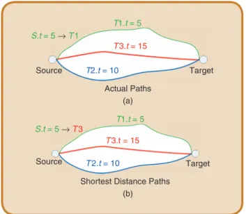
path. As mentioned earlier, one common approach for choos-ing such a path is based on the shortest distance criterion [1], [4]–[8], which fails in some situations (see Figure 2).
According to Wardrop’s Principles [10], the traffic in congested networks would move in a way such that no ve-hicle can reduce its travel cost by switching routes. This state is called user equilibrium, and is a result of every user non-collaboratively attempting to minimize the traveling cost—which commonly appears to be the travel time. Un-der such an equilibrium state, the average travel time is balanced for all users of the network.
Assumption: Based on these principles and the obser-vation that modern GPS largely adopts the fastest route planning strategy, we assume all GPS traces are planned using the shortest travel time criterion.
Denoting the network with true traffic conditions as ,
Gture all GPS traces represent the fastest routes planned on Gture. However, as we don’t have Gture, our goal is to use available GPS traces and an initial road network Gest, with all road segments set to their speed limits, to estimate
Gture or, in other words, to recon-struct the velocity field of Gture.
Collorary 1: A GPS trace with travel time t matching a path gAp h implies that no path in Gture from
g to h has a travel time smaller than .t
Proof: By our Assumption above, the traffic along every traveled route between g and h in Gture is in user equilibrium, and all routes have equivalent travel times. A travel time value for one path be-tween g and h thus provides a lower bound for the travel times of all paths.
Collorary 2: A pair of GPS points from a trace matched to locations g and h are sufficient to bound the travel time for paths between g and .h
Proof: By the Assumption, the path indicated by a GPS trace is a time-optimal path. Therefore, it has an optimal substructure. A subset of two is thus time-optimal and can provide a bound on the travel time for paths from g to .h
As Collorary 2 implies, during reconstruction of the ve-locity field we can inspect two consecutive GPS points at a time (optimal substructure). Considering two arbitrary GPS points si and si 1+, the true path si s
p i 1 true
A + is the
fast-est path between si and si 1+ on Gture. By Collorary 1, the
travel time ptrue.t=si+1.t s t- i. is the lower bound of all travel times between the two points. Subsequently, we en-force the constraint that no path in Gest between si and si 1+ has a smaller travel time. If such a path pest exists, the
speeds of the road segments on pest should be decreased until pest.t$ptrue. .t We refer to such pest as an overesti-mated path as its speed is higher than it should be. In prac-tice, pest connects candidate nodes of si and si 1+ rather
than si and si 1+ themselves, and there exists a set of paths
{pest all} for si and si 1+, in which one is the “closest” to ptrue.
Denoting an arbitrary element in {pest all} as pest, ptrue, and pest are likely to contain different sets of road segments. If pest and ptrue happen to be the same path, then pest.t should be equal to ptrue. ,t otherwise pest.t should be larger than ptrue. .t Since there is no further information for us to estimate the excessive time of pest.t over ptrue. ,t we take a conservative approach by setting pest.t= ptrue. .t We refer to this process of removing overestimated paths in {pest all} as relaxation.
The relaxation will make all paths in {pest all} have the same travel time (i.e., ptrue.t). However, it is very difficult to deterministically derive the “closest” path to ptrue.t us-ing a sus-ingle GPS trace. To remedy this issue, we rely on the “collective intelligence” of multiple GPS traces with shared road segments. As these segments will get gradually updated during relaxation of each GPS trace, they will eventually assist in differentiating the paths that include them from other paths in terms of the travel time. An illustration of
S.t = 5 → T 1
T1.t = 5
T 3.t = 15
T2.t = 10
Source Target
Actual Paths (a)
S.t = 5 → T 3 T1.t = 5
T 3.t = 15
T 2.t = 10
Source Target
Shortest Distance Paths (b)
FIg 2 An example illustrating a failure using the shortest distance criterion
on map matching trace S to T1, T 2, or T 3. By matching travel time of trace
S and road conditions, the correct path T1 is identified (a). By using only
the shortest distance criterion, S is mismatched to T 3 (b).
this process using the travel time as measurements can be found in Figure 3. The relaxation is essentially a ful-fillment of Wardrop’s Principles, and is conducted in a greedy fashion: we repeatedly extract the fastest path in {pest all and relax it, until no path in {} pest all} has its travel time smaller than ptrue. .t Given that there may exist many paths connecting two nodes in a network, the number of elements in {pest all} could be large, which further leads to an expensive computation. A sub-network with a specified radius is extracted from the network, which encompasses
,
si si 1+, and their mapping candidates but no more. With
this approach, we greatly reduced the number of paths in {pest all} . The rationale behind this choice is through em pirical findings that a vehicle rarely takes an opposite direction or arbitrary long detour from one GPS point to the next one.
Theorem 1: The speed of a road segment is monotoni-cally decreasing during relaxation.
Proof: We prove this theorem by contradiction. Assume two overestimated paths pest1 and pest2 share a road segment
.
e Without loss of generality, considering relaxation of pest1 , the road segment e has its speed .e v decreased to .e vl and travel time .e t increased to .e tl so that pest1 .t=ptrue1 . .t Now, during relaxation of pest2 , .e vl and .e tl are subject to change. If instead of monotonically decreasing .e vl gets increased and .e tl gets decreased, then we have pest1 .t1ptrue1 .t which
invalidates the previous relaxation process and further contradicts Collorary 1.
Taking advantage of Theorem 1, further reduction in computation can be achieved by retaining reduced
S 1.t = 5 → T 1
S 2.t = 15 → T 2
T 3.t = 10
T 2.t = 15
Source 2
Source 1
Target 2
Target 1
T 1.t = 5
e
Final Estimated Network and Trace Matching Results After Relaxation of S 1 and S 2
(d)
S 1.t = 5 → T 1 or T 3
S 2.t = 15
T 3.t = 5
Target 2
Target 1
Source 2
Source 1
T 1.t = 5
e T2.tmin
Updated Network and Trace Matching Results After Relaxation of S 1
(c)
S 1.t = 5
S 2.t = 15
Target 2 Source 2
Source 1 e T 2.tmin Target 1 T 3.tmin
Initial Network with Traces S1 and S2
T 1.tmin
(b)
S 1.t = 5 → T 1
S 2.t = 15 → T 2
Source 2 Target 2
T 2.t = 15
T 3.t = 10
Target 1 Source 1
T 1.t = 5
e
Actual Network and Trace Matching Results (Unknown) (a)
FIg 3 An illustration of the relaxation process of two traces S1 and S 2. The actual traffic conditions and trace matching results are shown in the top left panel. The inputs listed in the top right panel contain the initial network and trace information (i.e., sources, targets, and travel time). After relaxation of
trace S1, paths T 1 and T 3 have their travel time increased from the minimum value to S1.t. While S1 can be matched to either T 1 or T 3, the situation is
resolved after relaxation of S 2 due to further increase in travel time of the road segment e.
Input: Initial estimated road network Gest=( , )V E with e v e v. = . max,6e E! ; GPS traces S={ , , };S1fSm Discretized time intervals { , , };1fD Maximum
distance for computing candidate nodes of a GPS point cDis; Maximum number of candidate nodes cNum
Output: Reconstructed road network Gest 1: foreach time interval d!( , , )1fD do: 2: Sd=ExtractGPSTraces S d( , )
3: foreach traceSjd!Sddo:
4: forconsecutive GPS points ,s si i+1!Sdj do:
5: radius dist s s( ,2i i 1) cDis
= + +
6: H=ExtractSubgraph G radius s s( ,est , ,i i+1)
7: C1=GetCandidateNodes H s cDis cNum( , ,i , )
8: C2=GetCandidateNodes H s( , i+1,cDis cNum, )
9: p t strue. = i+1.t s t- i.
10: Hrelax=RelaxNetwork H p t C C( , true. , , )1 2 11: Gest=UpdateNetwork G H( ,est relax)
12: returnGest
speeds of each path in {pest all} . To be specific, as {pest all} is generated for si and si 1+ in a sub-network, many paths
in {pest all will have shared road segments. Therefore, the } speed reduction in these road segments will make multiple paths in {pest all to have increased travel times. As a result, } the greedy process of relaxation is much more efficient than a brute-force enumeration.
The overall process is described in Algorithm 1. Sub-routines RelaxNetwork and Relaxation are specified in Algorithm 2 and 3, respectively. In particular, two types of paths are considered as outliers and are excluded from the
computation: one has a travel time shorter than its free-flow travel time and one has a travel time longer than the travel time under the jam density. The procedure Travel-TimeAllocation in Line 10 of Algorithm 3 is discussed next.
C. Travel Time Allocation
During relaxation, we need to address each overestimat-ed path pest between GPS points si and si 1+ by making
. . . . .
pestt=ptruet=si+1t s t- i Due to the low sampling rate, pest often spreads several road segments, and the aggre-gate travel time ptrue.t needs to be appropriately allocated to individual road segments of pest. To address this issue with respect to traffic flow analysis, we adopt and modify the solution proposed in [11].
According to [11], the travel time of a road segment e can be decomposed into three categories: free-flow trav-el time xe f, , congestion time xe c,, and stopping time xe s,. For an overestimated path pest, we denote its total free-flow travel time as Tf=Re p! estxe f, , total congestion time as
,
Tc=Re p! estxe c, total stopping time as Ts=Re p! estxe s,, and the allocation time as Ta=ptrue. .t To validate pest, we must have Tf+Tc+Ts=Ta. While Tf can be derived trivially as Tf=Re p! estxe f, =Re p! est^e len e v. / . maxh, the computations of Tc and Ts require additional considerations.
By assuming nearby road segments have similar traf-fic conditions, the path congestion level is defined as
/ .
w=^T Tc c+Tfh The minimum value wmin=0 is reached when the path can be traveled with the free-flow speed, and the maximum value wmax=^Tc,max/Tc,max+Tfh where Tc,max=Ta-Tf is reached when the path is congested but no more so that Ts=0. With a specific path congestion lev-el wmin#w#wmax, the probability that a certain degree of congestion occurred on pest is computed as:
( ) min , · ,
P w
T T
T T
w
1 , , 1
prev prev
max max c
a a
c c
=
+ +
) 3 (1)
where Tprevc,max and Tpreva represent the maximum congestion time and the allocation time of path sj s ,j 1 i.
p j 1 est prev
A + + # In
[11], pestprev denotes the path which has an allocation time longer than the jam-density travel time with maximum possible .j In this work, as we have addressed path outli-ers, pestprev indicates the path connecting s
i 1- and ,si which is the directly preceding path of pest. ( )P wc is defined un-der assumptions that first, when all variables are fixed, the probability of a specific level of congestion occurring increases as Tc,max increases; second, given a particular
,
Tc,max higher level congestions are less likely to appear than lower level congestions.
Next, the stopping likelihood function is defined for com-puting the probability of stopping. Since the original formu-la does not take estimated traffic conditions into account, we alter it to:
( ) ( ) .. ,
L, w w 1 e ke k max
s e =b + -b (2)
Input: A set of road segments E (initially contains all road segments in pest); Time budget T (initially set to p ttrue. )
Output: A set of relaxed road segments Erelax
1: avgSpeed Re ET e
= ! 2 average travel speed
2: Tl=T 2 store the time budget 3: foreach road segmente E! do: 4: ife v avgSpeed. # then
5: T T e t= - . 2 the leftover time budget 6: E E e= \{ }2 exclude e based on theorem 1 7: ifTl!T then2 some e have been excluded 8: Erelax=Relaxation E T^, h2 recursive call
9: else
10: Erelax=TravelTimeAllocation E T^, h
11: returnErelax
Algorithm 3 Relaxation
Input: Subgraph H; True travel time p ttrue. ; Candidate node sets C C1, 2 Output: Relaxed subgraph Hrelax
1: foreach noden1!C1do: 2: foreach noden2!C2do:
3: ifn1==n2 or distance( , )n n1 2 ==0then 4: continue 2 no valid path exists 5: pest=GetFastestPath H n n( , , )1 2 6: ifIsOutlier p( )est = =truethen 7: continue
8: while truedo: 9: iftest$ttruethen
10: break 2 not an overestimated path 11: ifNumberOfNodes p( )12then 12: break 2 not a valid path 13: Erelax=Relaxation p p t( ,est true. )
14: H UpdateNetwork H E= ( , relax)2 update travel times of H using Erelax 15: pest=GetFastestPath H n n( , , )1 2 2 get the shortest travel time
path between n1 and n2 on H 16: returnHrelax=H
where b is the weighting factor (set to 0.5 in this work),
and .e k is the estimated density as a result of possible previous relaxation (otherwise .e k=0). Equation 2 computes the likelihood by leveraging the path con-gestion level w and the road-segment concon-gestion level
. / . .
e k e kmax
^ h Intuitively, the road-segment congestion level becomes higher when the estimated density .e k approaches the jam density .e kmax. In order to derive
.
e k from the estimated speed . ,e v we utilize the Green-shield’s model [42]:
. . .. .
e k e kmax 1 e ve v max
= ` - j (3)
By having the stopping likelihood function, the prob-ability that a vehicle stopped on a particular road segment is stipulated by assuming the vehicle stops at most once on
pest as:
( ) ( ) ( ( )).
P, w L, w 1 L, w
,
s e s e s e
e pestj i
i i j
j
=
-!
!
%
(4)
With Equation (1) and (4), the congestion time on a single road segment is calculated by integrating all path congestion levels together as:
( ) ( )
, w
w
Q
P w P w
dw 1
, ,
,
e c w e f
s
c s e
e 0
max
x = x
-/
#
(5)where Qs w P wc( ) eP w dws e, ( ) 0
max R
=
#
is the normalizingfactor. After summing the congestion time of all road seg-ments Tc=Re p! estxe c,, the total stopping time can be de-rived easily by Ts=Ta-Tf-Tc. Finally, we can calculate the stopping time on each road segment using the follow-ing formula:
( ) ( )
. T P w P wQ dw
, ,
e s w s
s
c s e
0 max
x =
#
(6)To this point, we have solved the travel time allocation problem by having xe f,,xe c,, and xe s, for all road segments of pest and fulfilling Tf+Tc+Ts=Ta (i.e., pest.t=ptrue. ).t
D. Evaluation on A Synthetic Network Using Traffic Simulation
In order to evaluate our technique on estimating velocity field, we use a synthetic road network and an agent-based traffic simulator [43]. The road network is modeled as a grid with 5 × 5 intersections. By considering one hour as a time interval for a specific congestion level, a set of cars is routed and average travel times of all road segments are taken as the ground truth for this congestion level. All traces are simulated by randomly sampling nodes of the network as sources and targets using the fastest route strategy in the beginning of a time interval. As our method operates on size 2 subsets of GPS traces, we emit pairs of points at the source and target for each simulated trace. This choice
re-sembles the low sampling rate feature and enables us to in-corporate the travel-time allocation algorithm into testing. All road segments share the same setting: length of
m,
150 maximum speed at .17 88m s,/ and a maximum den-sity of 0.15 cars per meter. In total, 30 congestion levels are created by simulating 50 to 1500 vehicles in this road net-work with an increment of 50 vehicles per time interval. In addition, for each time interval, five tiers of the vehicle population, at 20%, 40%, 60%, 80%, and 100%, are used to generate GPS traces.
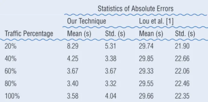
The first analysis is conducted by treating the network as a whole, and the aggregate travel time over the network is used to represent the global congestion level. The ground truth compared to estimated quantities using our technique and Lou et al. [1] are shown in Figure 4. Start with 20% of vehicles, our technique demonstrates close approxima-tion to the ground truth at all congesapproxima-tion levels, while such phenomena are not observed using the shortest- distance based technique developed in [1]. In Table 1, we examine each traffic percentage by computing the absolute error to the ground truth across all congestion levels. The smallest error (mean = 3.4s, std = 3.32s) is achieved by using 80% of GPS traces from the simulated traffic. The slight increase in error when using 100% GPS traces is mainly due to im-perfect travel-time allocation method.
In the second analysis, we computed relative improve-ments measured in mean squared error (MSE)1 of our method over [1]. The results are demonstrated in Figure 5.
In general, as the congestion level increases or a higher percentage of GPS traces becomes available, our tech-nique outperforms the shortest-distance techtech-nique. The improvements are less clear when congestion level is low (i.e., 110), but better seen when congestion approaches high level (i.e., 10$ ). The smaller improvement at the low-congestion levels is because when vehicles can travel on roads with speeds close to the speed limits, the shortest travel-time path and the shortest-distance path tend to be the same in such cases.
IV. Missing Value Completion
The temporal sparsity of GPS data can lead to missing val-ues in certain time intervals over a weekly period, and these missing values inhibit the accurate estimation of full traffic dynamics. To address this issue, we explore the sparse structure embedded in traffic patterns and propose a novel technique based on the Compressed Sensing algo-rithm [12], [13].
We have adopted loop-detector data2, which represent complete and relatively accurate measurements of traffic conditions, to explore features of traffic patterns. We use speed measurements from 38 loop detectors installed in
1MSE is computed as /1n (e t e t. . ) .
i n
1 2
R= t
-^ h
2The loop-detector data are obtained from Caltrans Performance
San Francisco. The time range of these data is the same as that of the Cabspotting data set3, which we adopted to estimate traffic conditions of San Francisco. We refer to the average speed measurements over a weekly period (discretized hourly) as a traffic signal. An example traffic signal exhibiting clear periodicity is shown in the top panel of Figure 6.
3http://cabspotting.org/.
We perform a spectral analysis on a traffic signal. In the analysis, we set the frequencies as the reciprocal of the signal length (i.e., 1/168) and subtract the signal from its mean to make the oscillations easier to observe. The results, which are shown in the middle panel of Figure 6, reveal that the period of the most salient oscillation is 24 hours. In addition, the signal exhibits sparsity in the frequency do-main, which is reflected as over 95% energy is preserved by retaining the ten largest frequencies ( Figure 6, BOTTOM).
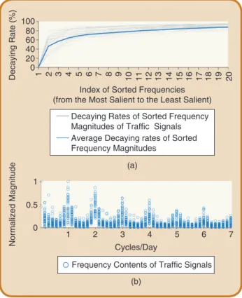
According to the specification of a traffic signal, the high-est frequency being supported is one cycle per two hours. To recover a traffic signal from its samples, the Nyquist-Shan-non Theorem says that we need at least 168 measurements. This number of samples is difficult to obtain because of the temporal sparsity of GPS data. However, the Compressed Sensing algorithm [12], [13] suggests that a signal can be recovered exactly with a small set of samples if the signal has a sparse representation. This sparse representation can be manifested by the rapid decaying of the sorted frequency magnitudes. The analysis of decay rates of traffic signals is presented in the top panel of Figure 7. On average, the decay rate reaches 45.78% with the most prominent frequency and 78.93% with the ten most conspicuous frequencies. After the 15th frequency, the decay rates become ineligible.
Another merit of Compressed Sensing is that it does not require any prior knowledge of the sparse structure of a
140 120 100 80 60 40 20 0
1 2 3 4 5 6 7 8 9 10 11 12 13 14 15 16 17 18 19 20 21 22 23 24 25 26 27 28 29 30
140 120 100 80 60 40 20 0
Average Travel
Time of the Network (s)
Average Travel
Time of the Network (s)
True Travel Time and Travel Time Computed Using Various Percentages of the Traffic Population (Our Technique)
True Travel Time and Travel Time Computed Using Various Percentages of the Traffic Population (Shortest Distance)
Congestion Level: Each Level Corresponds to (50 × Level Number) Cars Being Routed in the Network
True Time 20% 40% 60% 80% 100%
True Time 20% 40% 60% 80% 100%
(a)
1 2 3 4 5 6 7 8 9 10 11 12 13 14 15 16 17 18 19 20 21 22 23 24 25 26 27 28 29 30 (b)
FIg 4 Average travel time simulated on the synthetic road network using our approach (a) vs. [1] with the shortest distance (b). Our technique consistently outperforms the existing method in estimating the average travel time over 30 different congestion levels.
Statistics of Absolute Errors
Our Technique Lou et al. [1]
Traffic Percentage Mean (s) Std. (s) Mean (s) Std. (s)
signal. Since the road condition is intrinsically stochastic, the sparse structure of a traffic signal varies from one link to another. This phenomenon is demonstrated in the bot-tom panel of Figure 7, in which locations and amplitudes of the frequency components of all traffic signals are plot-ted. Besides the appearance of the prominent oscillations, at 24, 48, and 72 hours, other oscillations are spread out along the frequency axis. Together, these observations and features confirm the applicability of using Compressed Sensing to recover traffic signals.
Given a signal f!Rn and its measurements b!Rm, we consider the undersampled case in which the number of measurements m is smaller than the signal’s dimension
.
n The goal is to derive an estimated signal ft!Rn from b!Rm such that the error ||f f||
L2
- t is minimized. In gen-eral, the better the desired reconstruction quality, the more measurements are needed. In order to achieve a predefined accuracy level, signal reconstruction requires a minimum number of measurements mmin. According to [44], mmin is on the order of n2Slog( ),n where n is the coherence be-tween a measurement basis and a representation basis, S is the signal’s sparsity level, and n is the signal’s dimen-sion (in this work n=168). We estimate S by averaging the number of frequencies in preserving 95% energy of all traffic signals, which results in S=17 63. . The minimum coherence value n=1 is obtained by performing a discrete cosine transform (DCT) on a traffic signal f :
, fdct f
U = (7)
where fdct is the representation of f in the DCT domain and Un n# is the DCT matrix. With these estimated values,
Various Percentages of the Traffic Population Sending GPS Reports 0.6
0.5
0.4
0.3
0.2
0.1
0
1 2 3 4 5 6 7 8 9 10 11 12 13 14 15 16 17 18 19 20 21 22 23 24 25 26 27 28 29 30
Relative Improvement of Our Technique in MSE
Congestion Level
Various Percentages of the Traffic Population Sending GPS Reports
20% 40% 60% 80% 100%
FIg 5 Relative improvements measured in MSE of our technique over Lou et al. [1]. Our technique outperforms [1] as the congestion level increases or as more GPS traces become available. Our method achieves up to 52.5% improvement.
32 30 28 26
24 48 72 96
Time (h)
120 144 168
Speed (m/s)
Loop Detector Data Traffic Signal
(a)
1
0.5
0
1 2 3 4 5 6 7
Cycles/Day
Nor
maliz
ed
Magnitude
Frequency Contents of the Traffic Signal (b)
24 48 72 96
Time (h)
120 144 168
32 30 28 26
Speed (m/s)
Traffic Signal
Fitted Model with Ten Salient Frequencies (c)
FIg 6 The average speed measurements from loop-detector data are interpreted
as a traffic signal, which exhibits a clear periodic pattern (a); the spectral analysis
the minimum number of samples required to recover a traffic signal can be computed as: mmin= n2Slog( )n =
. log( ) .
1 17 632· · 168 .90
We test the performance of our method of signal re-covery by first obtaining random measurements via sam-pling: bm#1=Wm n n# f #1, where W is the sampling matrix constructed by randomly permuting rows of the identity matrix. Then we derive the recovered signal in the DCT domain fdctt from b by solving the following linear system:
.
A ftdct= WUftdct=b (8) Equation 8 represents an underdetermined system, in which there exist infinitely many candidate signals fdctt for which the formula can suffice. Among all candidates, the desired fdctt should exhibit sparsity as observed in fdct. We can acquire such a solution by solving the following opti-mization program:
, min fdctt L1
. A f b.
s.t tdct= (9)
An example solution to Equation 9 is shown in Figure 8, where the actual solution elements of fdct and the recovered
solution elements of fdctt both demonstrate sparsity. The final recovered signal ft is acquired by performing an inverse DCT on fdctt . Figure 9 gives an example in which the recovered sig-nal exhibits high similarity to the origisig-nal sigsig-nal. A more thor-ough analysis of the performance of recovering traffic signals can be found in Figure 10. As a result, both the standard de-viation and the expectation of the L2 loss decrease, when the number of measurements used in recovery increases. The av-erage error of using 90 measurements is 1.4 m/s.
To put this framework in terms of GPS data, the measure-ments used are obtained from travel time estimation rather than from the sampling operation that we performed on a traffic signal. In this case, U is set to DCT diag 1^ ^ , ,f1hh, and A=WD is taken to solve Equation 9. Since we have established that mmin=90, it is worth mentioning that we only address links that have measurements in more than 90 time intervals. Compared to [45] and [9], we have re-duced the minimum number of measurements required to recover a traffic signal from 1680 to 90 (by 94.64%).
V. Estimating Traffic Dynamics Via gPS Data
One of the hallmarks of traffic dynamics is their periodic-ity [9]: traffic patterns show a clear trend over the course of a day and collectively over the course of a week. In this
150
120
90
60
30
1
Number of Solution Elements
–20 –16 –12 –8 –4 0 4 8 12 16 20
Values of Solution Elements (Actual) 150
120
90
60
30
1
Number of Solution Elements
–20 –16 –12 –8 –4 0 4 8 12 16 20
Values of Solution Elements (L1 Norm)
FIg 8 Solution elements (in total 168) by solving an underdetermined
system via convex optimization. Both the actual and the L1-norm based
recovery demonstrate sparsity (i.e., most solution elements are approximately equal to zero).
100 80 60 40 20 0
1 2 3 4 5 6 7 8 9 10 11 12 13 14 15 16 17 18 19 20
Decaying Rate (%)
Index of Sorted Frequencies (from the Most Salient to the Least Salient)
Decaying Rates of Sorted Frequency Magnitudes of Traffic Signals Average Decaying rates of Sorted Frequency Magnitudes
(a) 1
0.5
0
1 2 3 4
Cycles/Day
5 6 7
Normalized Magnitude
Frequency Contents of Traffic Signals (b)
section, we first demonstrate that this phenomenon can be recovered using our technique (tested on the Cabspotting data set); we then analyze features revealed in the recon-structed traffic patterns.
To assist in visualization and analysis, the metric fluid-ity, adapted from [9], is used for each road segment as the ratio of the estimated travel speed to the free-flow speed. this metric ranges from 0 to 1. In Figure 11, we show the estimated traffic dynamics, denoted by average fluidity, across the road network of downtown San Francisco. From the demonstration, it is clear that our technique recovers the periodicity of the traffic pattern using the dominant frequency, which is one cycle per day. This characteristic resembles the one observed in loop-detector data from the same area (see Figure 6 and 9).
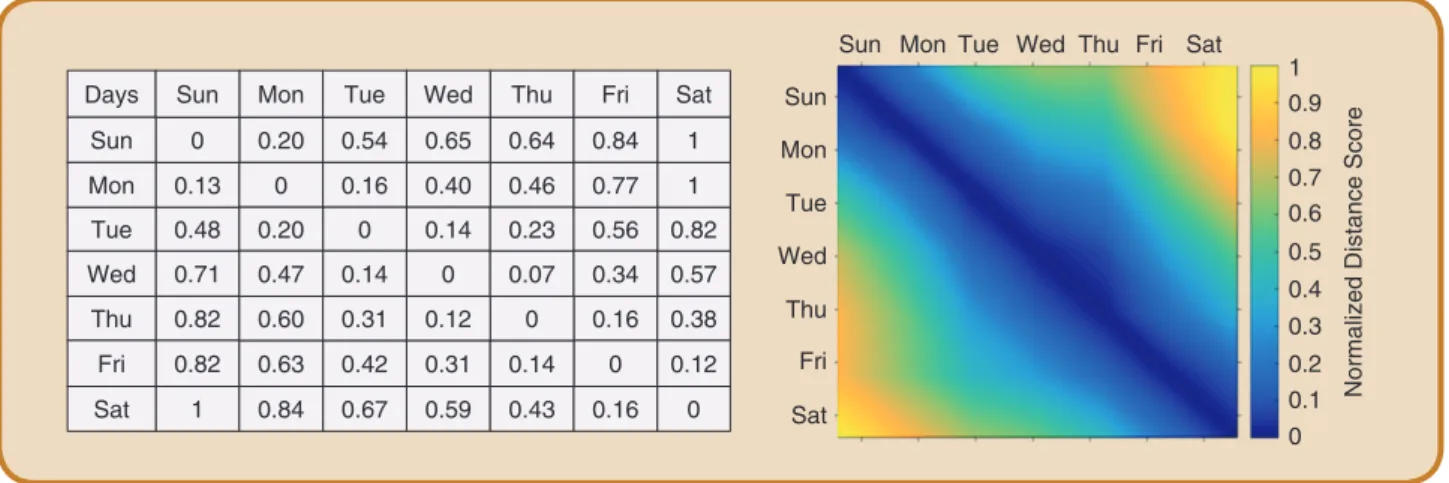
The affinity between different days in a week can also be used to illustrate the quality of our data reconstruction method. We compute the correlation of every pair of days using the cosine distance for both the estimated traffic conditions and the actual conditions derived from loop-detector data. In Figure 12, left panel, we provide all dis-tance scores: the upper triangular matrix is derived using the estimated values, and the lower triangular matrix is computed using loop-detector data. In the right panel of Figure 12, we provide the qualitative result for a visual inspection. The symmetrical pattern across the diagonal line indicates that the estimated traffic states largely agree with the loop-detector data.
Based on the distance scores, a hierarchical clustering is performed to reveal the similarity between day pairs.
The closest pair is Wednesday and Thursday, followed by Friday and Saturday, and Monday and Tuesday. In the sec-ond level of the hierarchy, Sunday joins Msec-onday and Tues-day. These three day-pairs suggest that a typical week of San Francisco can be roughly divided into three stages: beginning of the week (Sunday, Monday, and Tuesday), middle of the week (Wednesday and Thursday), and end of the week (Friday and Saturday).
VI. Conclusion
We have presented a novel computational scheme for esti-mating travel times, traversed paths, and missing values
32 30 28 26
24 48 72 96 120 144 168
24 48 72 96 120 144 168
32 30 28 26
Speed (m/s)
Speed (m/s)
Time (h)
Time (h)
Recovered Signal-Using L1 Norm as the Constraint Actual Traffic Signal Sample Measurements
(a)
(b)
FIg 9 Recovery of a traffic signal via Compressed Sensing. The actual
signal and its 90 random measurements are plotted (a). The L1-norm
based recovery (b) shows high similarity to the actual signal.
10 9 8 7 6 5 4 3 2 1 0
12 24 36 48 60 72 84 96 108 120 132 144 156 168
L2-Norm Loss (m/s)
Number of Samples Used in Signal Recovery Errors in Recovering Traffic Signals Average Errors in Recovering Traffic Signals
FIg 10 The error between recovered and actual traffic signals. As more samples are used in signal’s recovery, we observe smaller errors.
Fluidity
1
0.5
0
1
0.5
0 24
1 2 3 4
Cycles/Day
5 6 7
48 72 96 120 144 168
Time (h)
Nor
maliz
ed
Magnitude
Frequency Contents of the Averaged Traffic Dynamics Estimation of Averaged Traffic Dynamics
over a large-scale road network using spatially and tem-porally sparse GPS traces. Specifically, an approach based on the shortest travel time is performed to reconstruct the velocity field of a road network. As a result, we have obtained a novel method for joint estimation of traversed paths and travel times on a large-scale road network. Next, an algorithm based on the Compressed Sensing algorithm has been developed to estimate missing travel information over an entire traffic period so that citywide traffic dynam-ics can be studied. Last, we have extensively evaluated our approach and compared our technique with a state-of-the-art technique. Consistent improvements are observed in multiple traffic scenarios.
There are several possible future directions. To start with, as abundant GPS data are becoming available, the task of processing them is computationally expensive. Be-sides using the power of distributed computing, it is promis-ing to explore the sparse structure and periodicity of traffic patterns to further reduce the amount of data needed in the estimation of traffic dynamics. Similarly, correlation in traffic patterns due to proximity/spatial coherence can also be examined. Last, it might be beneficial to integrate data mining of historical data, real-time traffic reconstruc-tion from current data, and predictive traffic simulareconstruc-tion to achieve a more comprehensive and accurate estimation of travel conditions over metropolitan areas.
About the Authors
Weizi Li received his B.E. degree in
Computer Science and Technology from Xiangtan University, China and M.S. de-gree in Computer Science from George Mason University. He is currently in the doctoral program at the University of North Carolina at Chapel Hill,
De-partment of Computer Science. His research interests include agent-based simulation, intelligent transportation systems, and statistical machine learning.
Dong Nie received his B.Eng. degree in
Software Engineering from Northeast-ern University, Shenyang, China and M.Sc. degree in Computer Science from the University of Chinese Academy of Sciences, Beijing, China. He is pursu-ing a Ph.D. degree in Computer Sci-ence from the University of North Carolina at Chapel Hill. His research interests include image processing and medi-cal image analysis.
David Wilkie received a BS in
compu-ter science from Drexel University and his PhD from the University of North Carolina at Chapel Hill, Department of Computer Science. He is now a software engineer for Google Maps. David’s re-search interests include traffic simu-lation, GIS and road network modeling, and intelligent transportation systems.
Ming C. Lin received her B.S., M.S.,
Ph.D. degrees in Electrical Engineer-ing and Computer Science from the University of California, Berkeley. She is currently John R. & Louise S. Parker Distinguished Professor of Computer Science at the University of North Car-olina (UNC), Chapel Hill. She has received several hon-ors and awards, including the NSF Young Faculty Career Award, UNC Hettleman Award for Scholarly Achievements,
Days Sun
Sun
Sun
Sun Mon Tue Wed Thu Fri Sat 1 0.9 0.8 0.7 0.6 0.5 0.4 0.3 0.2 0.1 0 Mon
Tue
Wed
Thu
Fri
Sat Mon
Mon
Tue
Tue
Wed
Wed
Thu
Thu
Fri
Fri
Sat
Sat 0 0.13
0.20 0.54 0.65 0.64
0.46 0.23 0.07
0.14
0.43 0.16
0.16 0.34
0.56 0.82
0.57 0.38 0.12 0.77
0.84 1
1 0.40
0.14
0.12 0.31 0.59 0.20
0.47 0.60 0.63 0.84
0 0.16
0.14 0.31 0.42 0.67 0
0 0
0 0 0.48
0.71 0.82 0.82
1 Normalized Distance Score
2010 IEEE VGTC Technical Achievement Award, and 10 best paper awards at premium international conferences. She is a Fellow of ACM and IEEE.
She has served as a member of the Board of Directors of Computing Research Association Women, a member of IEEE CS Board of Governors, Chair of 2015 IEEE Computer Society (CS) Transactions Operation Committee, and a for-mer Editor-in-Chief of IEEE Transactions on Visualization and Computer Graphics (2011–2014). She is also a mem-ber of several Editorial Boards, steering committees, and advisory boards of international conferences, government agencies, and industry.
References
[1] Y. Lou, C. Zhang, Y. Zheng, X. Xie, W. Wang, and Y. Huang, “Map-matching for low-sampling-rate GPS trajectories,” in Proc. 17th ACM SIGSPATIAL Int. Conf. Advances in Geographic Information Systems. ACM, 2009, pp. 352–361.
[2] D. Schrank, B. Eisele, T. Lomax, and J. Bak, “2015 urban mobility scorecard,” Texas A&M Transportation Institute and INRIX, 2015. [3] G. Leduc, “Road traffic data: Collection methods and applications,”
Work-ing Papers on Energy, Transport and Climate Change, vol. 1, no. 55, 2008. [4] J. Yuan, Y. Zheng, C. Zhang, X. Xie, and G. Sun, “An interactive-voting based map matching algorithm,” in Proc. 11th Int. Conf. Mobile Data Management, 2010, pp. 43–52.
[5] T. Miwa, D. Kiuchi, T. Yamamoto, and T. Morikawa, “Development of map matching algorithm for low frequency probe data,” Transp. Res. Part C Emerg. Technol., vol. 22, pp. 132–145, 2012.
[6] T. Hunter, P. Abbeel, and A. Bayen, “The path inference filter: Model-based low-latency map matching of probe vehicle data,” IEEE Trans. Intell. Transp. Syst., vol. 15, no. 2, pp. 507–529, 2014.
[7] B. Y. Chen, H. Yuan, Q. Li, W. H. Lam, S.-L. Shaw, and K. Yan, “Map-matching algorithm for large-scale low-frequency floating car data,” Int. J. Geogr. Inf. Sci., vol. 28, no. 1, pp. 22–38, 2014.
[8] M. Quddus and S. Washington, “Shortest path and vehicle trajectory aided map-matching for low frequency GPS data,” Transp. Res. Part C Emerg. Technol., vol. 55, pp. 328–339, 2015.
[9] A. Hofleitner, R. Herring, A. Bayen, Y. Han, F. Moutarde, and A. D La Fortelle, “Large scale estimation of arterial traffic and structural analysis of traffic patterns using probe vehicles,” in Proc. Transporta-tion Research Board 91st Annu. Meeting, 2012.
[10] J. Wardrop, “Some theoretical aspects of road traffic research,” in Proc. Inst. Civ. Eng., vol. 1, no. 3, pp. 325–362, 1952.
[11] B. Hellinga, P. Izadpanah, H. Takada, and L. Fu, “Decomposing travel times measured by probe-based traffic monitoring systems to individ-ual road segments,” Transp. Res. Part C Emerg. Technol., vol. 16, no. 6, pp. 768–782, 2008.
[12] D. Donoho, “Compressed sensing,” IEEE Trans. Inf. Theory, vol. 52, no. 4, pp. 1289–1306, 2006.
[13] E. Candes, J. Romberg, and T. Tao, “Robust uncertainty principles: ex-act signal reconstruction from highly incomplete frequency informa-tion,” IEEE Trans. Inf. Theory, vol. 52, no. 2, pp. 489–509, 2006. [14] H. B. Celikoglu, “A dynamic network loading model for traffic
dynam-ics modeling,” IEEE Trans. Intell. Transp. Syst., vol. 8, no. 4, pp. 575– 583, 2007.
[15] H. B. Celikoglu, E. Gedizlioglu, and M. Dell’Orco, “A node-based mod-eling approach for the continuous dynamic network loading problem,” IEEE Trans. Intell. Transp. Syst., vol. 10, no. 1, pp. 165–174, 2009. [16] S. Gao, “Modeling strategic route choice and real-time information
impacts in stochastic and time-dependent networks,” IEEE Trans. In-tell. Transp. Syst., vol. 13, no. 3, pp. 1298–1311, 2012.
[17] A. Abadi, T. Rajabioun, and P. A. Ioannou, “Traffic flow prediction for road transportation networks with limited traffic data,” IEEE Trans. Intell. Transp. Syst., vol. 16, no. 2, pp. 653–662, 2015.
[18] P. Kachroo and S. Sastry, “Travel time dynamics for intelligent trans-portation systems: Theory and applications,” IEEE Trans. Intell. Transp. Syst., vol. 17, no. 2, pp. 385–394, 2016.
[19] S. Agarwal, P. Kachroo, and S. Contreras, “A dynamic network mod-eling-based approach for traffic observability problem,” IEEE Trans. Intell. Transp. Syst., vol. 17, no. 4, pp. 1168–1178, 2016.
[20] D. Work, S. Blandin, O.-P. Tossavainen, B. Piccoli, and A. Bayen, “A traffic model for velocity data assimilation,” Appl. Math. Res. Exp., vol. 2010, no. 1, pp. 1–35, 2010.
[21] Y. Sun and D. Work, “A distributed local kalman consensus filter for traffic estimation,” in Proc. 53rd IEEE Annual Conf. Decision and Con-trol, 2014, pp. 6484–6491.
[22] A. Gning, L. Mihaylova, and R. K. Boel, “Interval macroscopic models for traffic networks,” IEEE Trans. Intell. Transp. Syst., vol. 12, no. 2, pp. 523–536, 2011.
[23] L. Li, X. Chen, and L. Zhang, “Multimodel ensemble for freeway traffic state estimations,” IEEE Trans. Intell. Transp. Syst., vol. 15, no. 3, pp. 1323–1336, 2014.
[24] H. B. Celikoglu and M. A. Silgu, “Extension of traffic flow pattern dy-namic classification by a macroscopic model using multivariate clus-tering,” Transp. Sci., 2016.
[25] M. Hajiahmadi, G. S. van de Weg, C. M. Tampère, R. Corthout, A. He-gyi, B. De Schutter, and H. Hellendoorn, “Integrated predictive control of freeway networks using the extended link transmission model,” IEEE Trans. Intell. Transp. Syst., vol. 17, no. 1, pp. 65–78, 2016. [26] A. Phan and F. P. Ferrie, “Interpolating sparse GPS measurements
via relaxation labeling and belief propagation for the redeployment of ambulances,” IEEE Trans. Intell. Transp. Syst., vol. 12, no. 4, pp. 1587–1598, 2011.
[27] Q.-J. Kong, Q. Zhao, C. Wei, and Y. Liu, “Efficient traffic state estima-tion for large-scale urban road networks,” IEEE Trans. Intell. Transp. Syst., vol. 14, no. 1, pp. 398–407, 2013.
[28] J.-D. Zhang, J. Xu, and S. S. Liao, “Aggregating and sampling meth-ods for processing GPS data streams for traffic state estimation,” IEEE Trans. Intell. Transp. Syst., vol. 14, no. 4, pp. 1629–1641, 2013. [29] J. Tang, Y. Song, H. Miller, and X. Zhou, “Estimating the most likely
space–time paths, dwell times and path uncertainties from vehi-cle trajectory data: A time geographic method,” Transp. Res. Part C Emerg. Technol., vol. 66, pp. 176–194, 2016.
[30] M. Rahmani and H. Koutsopoulos, “Path inference from sparse float-ing car data for urban networks,” Transp. Res. Part C Emerg. Technol., vol. 30, pp. 41–54, 2013.
[31] M. Rahmani, E. Jenelius, and H. Koutsopoulos, “Non-parametric esti-mation of route travel time distributions from low-frequency floating car data,” Transp. Res. Part C Emerg. Technol., vol. 58, pp. 343–362, 2015.
[32] A. Khosravi, E. Mazloumi, S. Nahavandi, D. Creighton, and J. Van Lint, “Prediction intervals to account for uncertainties in travel time pre-diction,” IEEE Trans. Intell. Transp. Syst., vol. 12, no. 2, pp. 537–547, 2011.
[33] B. Westgate, D. Woodard, D. Matteson, and S. Henderson, “Travel time estimation for ambulances using bayesian data augmentation,” Ann. Appl. Stat., vol. 7, no. 2, pp. 1139–1161, 2013.
[34] R. Herring, A. Hofleitner, P. Abbeel, and A. Bayen, “Estimating arte-rial traffic conditions using sparse probe data,” in Proc. 13th Int. IEEE Conf. Intelligent Transportation Systems, 2010, pp. 929–936. [35] A. Hofleitner, R. Herring, P. Abbeel, and A. Bayen, “Learning the
dy-namics of arterial traffic from probe data using a dynamic bayesian network,” IEEE Trans. Intell. Transp. Syst., vol. 13, no. 4, pp. 1679– 1693, 2012.
[36] K. Kuhi, K. K. Kaare, and O. Koppel, “Using probabilistic models for missing data prediction in network industries performance measure-ment systems,” in Proc. Eng., vol. 100, pp. 1348–1353, 2015.
[37] Y. Wang, Y. Zheng, and Y. Xue, “Travel time estimation of a path using sparse trajectories,” in Proc. 20th ACM SIGKDD Int. Conf. Knowledge Discovery and Data Mining, 2014, pp. 25–34.
[38] M. T. Asif, N. Mitrovic, J. Dauwels, and P. Jaillet, “Matrix and tensor based methods for missing data estimation in large traffic networks,” IEEE Trans. Intell. Transp. Syst., vol. 17, no. 7, pp. 1816–1825, 2016. [39] Y. Zhu, Z. Li, H. Zhu, M. Li, and Q. Zhang, “A compressive sensing
ap-proach to urban traffic estimation with probe vehicles,” IEEE Trans. Mob. Comput., vol. 12, no. 11, pp. 2289–2302, 2013.
[40] N. Mitrovic, M. T. Asif, J. Dauwels, and P. Jaillet, “Low-dimensional mod-els for compressed sensing and prediction of large-scale traffic data,” IEEE Trans. Intell. Transp. Syst., vol. 16, no. 5, pp. 2949–2954, 2015. [41] O. Anava, E. Hazan, and A. Zeevi, “Online time series prediction with
missing data,” in Proc. 32nd Int. Conf. Machine Learning, 2015, pp. 2191–2199.
[42] B. Greenshields, J. Bibbins, W. Channing, and H. Miller, “A study of traf-fic capacity,” Highw. Res. Board Proc., vol. 14, no. 1, pp. 448–477, 1935. [43] D. Krajzewicz, J. Erdmann, M. Behrisch, and L. Bieker, “Recent
devel-opment and applications of SUMO–simulation of urban mobility,” Int. J. Adv. Syst. Measure., vol. 5, no. 3/4, pp. 128–138, 2012.
[44] E. Candès and M. Wakin, “An introduction to compressive sampling,” IEEE Signal Process. Mag., vol. 25, no. 2, pp. 21–30, 2008.