The University of Sydney Business School The University of Sydney
BUSINESS ANALYTICS WORKING PAPER SERIES
GEL Estimation for Heavy-Tailed GARCH
Models with Robust Empirical Likelihood
Inference
Jonathan B. Hill
University of North Carolina Chapel Hill
Artem Prokhorov
University of Sydney
September 10, 2015
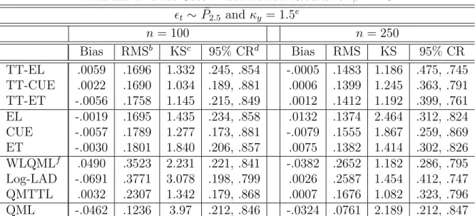
We construct a Generalized Empirical Likelihood estimator for a GARCH(1,1) model with a possibly heavy tailed error. The estimator imbeds tail-trimmed estimating equations allowing for over-identifying conditions, asymptotic normality, efficiency and empirical likelihood based confidence regions for very heavy-tailed random volatility data. We show the implied probabilities from the tail-trimmed Continuously Updated Estimator elevate weight for usable large values, assign large but not maximum weight to extreme observations, and give the lowest weight to non-leverage points. We derive a higher order expansion for GEL with imbedded tail-trimming (GELITT), which reveals higher order bias and efficiency properties, available when the GARCH error has a finite second moment. Higher order asymptotics for GEL without tail-trimming requires the error to have moments of substantially higher order. We use first order asymptotics and higher order bias to justify the choice of the number of trimmed observations in any given sample. We also present robust versions of Generalized Empirical Likelihood Ratio, Wald, and Lagrange Multiplier tests, and an efficient and heavy tail robust moment estimator with an application to expected shortfall estimation. Finally, we present a broad simulation study for GEL and GELITT, and demonstrate profile weighted expected shortfall for the Russian Ruble - US Dollar exchange rate. We show that tail-trimmed CUE-GMM dominates other estimators in terms of bias, mse and approximate normality.
Key words and phrases: GEL, GARCH, tail trimming, heavy tails, robust inference, efficient moment estimation, expected shortfall, Russian Ruble.
AMS classifications : 62M10 , 62F35. JEL classifications : C13 , C49.
BA Working Paper No: BAWP-2015-03
GEL Estimation for Heavy-Tailed GARCH
Models with Robust Empirical Likelihood
Inference
Jonathan B. Hill
∗University of North Carolina – Chapel Hill
Artem Prokhorov
†University of Sydney
September 10, 2015
Abstract
We construct a Generalized Empirical Likelihood estimator for a GARCH(1,1) model with a possibly heavy tailed error. The estimator imbeds tail-trimmed estimating equations allowing for over-identifying conditions, asymptotic normality, efficiency and empirical like-lihood based confidence regions for very heavy-tailed random volatility data. We show the implied probabilities from the tail-trimmed Continuously Updated Estimator elevate weight for usable large values, assign large but not maximum weight to extreme observations, and give the lowest weight to non-leverage points. We derive a higher order expansion for GEL with imbedded tail-trimming (GELITT), which reveals higher order bias and efficiency properties, available when the GARCH error has a finite second moment. Higher order asymptotics for GEL without tail-trimming requires the error to have moments of sub-stantially higher order. We use first order asymptotics and higher order bias to justify the choice of the number of trimmed observations in any given sample. We also present robust versions of Generalized Empirical Likelihood Ratio, Wald, and Lagrange Multiplier tests, and an efficient and heavy tail robust moment estimator with an application to expected shortfall estimation. Finally, we present a broad simulation study for GEL and GELITT, and demonstrate profile weighted expected shortfall for the Russian Ruble - US Dollar ex-change rate. We show that tail-trimmed CUE-GMM dominates other estimators in terms of bias, mse and approximate normality.
Key words and phrases: GEL, GARCH, tail trimming, heavy tails, robust inference, effi-cient moment estimation, expected shortfall, Russian Ruble.
AMS classifications : 62M10 , 62F35.
JEL classifications : C13 , C49.
∗Corresponding author. Dept. of Economics, University of North Carolina, Chapel Hill, NC;
http://www.unc.edu/∼jbhill; [email protected]
†The University of Sydney Business School and St.Petersburg State University;
1
Introduction
We develop a Generalized Empirical Likelihood estimator for a potentially very heavy tailed GARCH(1,1) process by tail-trimming estimating equations. The setting is motivated by recent
intense interest in information theoretic methods (Smith, 1997; Imbens, 1997; Kitamura, 1997;
Antoine, Bonnal, and Renault, 2007), including the higher order properties of GEL estimators
(Newey and Smith, 2004; Anatolyev, 2005), coupled with empirical evidence that the
distribu-tions of many financial returns have very heavy tails (e.g. Embrechts, Kluppleberg, and Mikosch,
1997; Wagner and Marsh, 2005; Ibragimov, 2009; Hill, 2015b) and exhibit volatility clustering
(Bollerslev, 1986).
The time series of interest is a stationary ergodic scalar process {yt}with increasing σ-fields
=t ≡ σ({yτ}:τ ≤t) and a strong-GARCH(1,1) representation
yt =σtt wheret is iid, E[t] = 0 and E[2t] = 1 (1)
σt2 =ω0+α0yt2−1+β0σ2t−1, where ω0 >0, α0, β0 ≥0, andα0 +β0 >0.
The assumption α0 + β0 > 0 safeguards against well known estimation boundary problems,
although allowing α0 = 0 and/or β0 = 0 merely requires an additional functional limit theory (Andrews, 1999; Francq and Zako¨ıan, 2004). Assume Θ is a compact subset of points θ =
[ω, α, β]0 that contains θ0 as an interior point, and the stationarity and ergodicity condition
E[ln(α+β2
t)] < ∞holds (Nelson, 1990; Bougerol and Picard, 1992):
Θ⊆
θ ∈(0,∞)×(0,1)×(0,1) :E
ln α+β2t
<∞ . (2)
We work with a linear strong-GARCH model solely to focus ideas and to motivate the use of
tail-trimming to deliver a robust GEL estimator. An extension of our methods to higher order
GARCH processes is trivial. In order to include a model of the conditional mean, however, a
more nuanced trimming approach is required since the relevant QML estimating equations may
have heavy tailed iterative terms which impact the resulting Jacobian in a more complicated way.
See Appendix B for a brief discussion concerning an ARMA-GARCH model.1 Our asymptotic
1We show how to construct trimmed estimating equations, and note that no additional moment conditions
on yt are required. Francq and Zako¨ıan (2004, Theorem 3.2), however, show that the QML estimator requires yt itself to have a finite fourth moment, a tremendous requirement in practice since many finanncial time series
theory relies heavily on uniform asymptotics for stationary mixing data,2 hence whether our
required results extend to non-stationary cases is not yet known.3
The iid assumption fortimplies our trimmed QML-type estimating equations are martingale differences. This simplifies estimation since smoothing is not required (cf. Owen, 1990, 1991; Kitamura, 1997; Kitamura and Stutzer, 1997), and this leads to sharp details concerning how
the implied probabilities relate information about usable sample extremes. Furthermore, the iid
assumption allows us to explicitly show how higher order bias is reduced by reducing trimming.
We can easily allow for weakly dependent errors by smoothing the estimating equations, but
the cost is far fewer details about how the smoothed implied probabilities translate information
about extremes, and essentially no information about how trimming impacts higher order bias.4
Since the latter two are key contributions in this paper, we simply focus on iid errors.
Construct volatility and error functions
σt2(θ) = ω+αy2t−1+βσt2−1(θ) and t(θ) = yt/σt(θ) where θ= [ω, α, β]
0
∈R3,
and letmt(θ) denote estimating equations based on{yt, σt(θ)}, a stochastic mapping mt : Θ →
Rq with q ≥ 3 that satisfies the global identification condition
E[mt(θ)] = 0 if and only if θ=θ0 for unique θ0 in compact Θ⊂R3.
In Section 2 we note that σ2
t(θ) is not observed, and utilize an iterated approximation.
We consider equations mt(θ) ∈ Rq,q ≥ 3, based on QML score equations, with added over-identifying restrictions based on stochastic weights wt(θ)∈ Rq−3. Hence, we use:
mt(θ) = 2t(θ)−1
×xt(θ)∈Rq,q ≥3, where xt(θ)≡[s0t(θ), w
0
t(θ)]
0
and st(θ)≡ 1
σ2
t(θ)
∂ ∂θσ
2
t(θ).
2See the proof of Lemma A.5 in the technical appendix Hill and Prokhorov (2014). This result is crucial for
showing the estimating equations{mˆ∗n,t(θ), m∗n,t(θ)}, defined below, satisfy supθ∈Θ||n−1/2Σ−1/2
n (θ)Pnt=1{mˆ∗n,t(θ) −m∗n,t(θ)}||=op(1), while a uniform limit is required since the tail-trimmed estimating equations are nonlinear
functions of θ. See especially the proof of Theorem 5.2 in Appendix A.4.
3Some uniform limit theory for QML score components in the nonstationary GARCH case is presented in
Jensen and Rahbek (2004b, Lemma 5) and Linton, Pan, and Wang (2010, Lemma 5). These arguments, how-ever, do not cover our required property supθ∈Θ{1/n1/2|Pn
t=1(si,t(θ)−E[si,t(θ)])|} = Op(1), where st(θ) ≡
(∂/∂θ) lnσt2(θ) andσt2(θ) =ω +αyt2−1 +βσt2−1(θ). We use a uniform limit theory in Doukhan, Massart, and Rio (1995) for stationary mixing data to prove the required results.
4This follows since higher order bias is a function of higher moments of tail-trimmed partial sums. These
Implicitly ifq = 3 thenxt(θ) =st(θ), whileq >3 aligns with over-identifying restrictionsE[(2t− 1)wi,t] = 0 fori= 1, ..., q−3. We assumewt(θ) is=t−1-measurable, continuous and differentiable.
Identification E[(2t − 1)xt] = 0 and E[2t] = 1 imply xt must be integrable, while st is square integrable when α0 + β0 > 0 (Francq and Zako¨ıan, 2004), hence we assume wt is integrable. Instrument classes other than QML-equations are obviously possible (cf. Skoglund, 2010). The
use of QML-equations is known to result in an efficient (exactly identified) GMM estimator in
the sense of Godambe (1985), cf. Li and Turtle (2000). Further, since the instrumentstis square integrable, ifxt contains only lags ofstthen heavy tail challenges arise solely due to the error t. Several recent papers consider properties of QML and LAD estimators of GARCH under
heavy tailed errors. Hall and Yao (2003) derive the QML estimator limit distribution for
linear GARCH when t belongs to a domain of attraction of stable law with tail exponent κ ∈ [2,4]. They show that the convergence rate isn1−2/κ/L(n) for slowly varying5 L(n)→ ∞, where
n1−2/κ/L(n)< n1/2 for anyκ∈[2,4]. See also Berkes and Horvath (2004) for consistency results. Although QML for GARCH is robust to heavy tails in possibly non-stationary yt, as long as t has a finite fourth moment, in small samples it is known to exhibit bias (e.g. Lumsdaine, 1995;
Gonzalez-Rivera and Drost, 1999; Berkes and Horvath, 2004; Jensen and Rahbek, 2004a).
A finite variance E[2
t] < ∞ appears indispensable for obtaining an asymptotically normal estimator. Linton, Pan, and Wang (2010) prove √n-convergence and asymptotic normality of
the log-LAD estimator arg minθ∈ΘPn
t=1|lny2t − lnσt2(θ)| for non-stationary GARCH provided
thas a zero median. See also Peng and Yao (2003) for earlier work with iid errors. Zhu and Ling (2011) show the weighted Laplace QML estimator is √n-convergent and asymptotically normal
if t has a zero median and E|t| = 1. They only require E[2t] < ∞, but in practice GARCH models are typically used under the assumption E[2t] = 1 irrespective of the estimator chosen. The classic assumption E[2
t] = 1 coupled with E|t| = 1 seems to severely limit the available distributions fort. Berkes and Horvath (2004) tackle non-Gaussian QML which for identification requires moment conditions either beyond, or in place of, the traditional E[t] = 0 and E[2t] = 1. Thus, in general these estimators are not technically for Bollerslev’s (1986) seminal GARCH
model (1) in which independence and E[2
t] = 1 imply identically σt2 = E[yt2|=t−1], and they
naturally do not allow for over-identifying restrictions.
Hill (2015a) uses a variety of trimming and weighting techniques for QML and method of
moments estimators for heavy tailed GARCH. However, over-identifying restrictions are not
allowed, profiles weights are not developed and therefore efficient moment estimators are not treated, and the empirical likelihood method for inference is not considered. See also Hill (2013)
for a related least squares theory for autoregressions. Notice, though, that moment conditions
not used for estimation can always be tested using heavy tail robust methods (Hill and Aguilar,
2013), while a large variety of model specification tests can be rendered heavy tail robust (Hill,
2012; Hill and Aguilar, 2013; Aguilar and Hill, 2015). Moreover, higher order asymptotics have evidently never been used for determining a reasonable negligible trimming strategy.
The present paper extends the line of heavy tail robust estimation and inference in Hill and
Aguilar (2013), Aguilar and Hill (2015) and Hill (2012, 2013, 2015a,b) to a GEL framework and to
the empirical likelihood method. As in those papers we apply a heavy tail robust, but negligible,
data transform to the estimating equations. We allow over identifying restrictions with one-step
estimation and inference that leads to Gaussian asymptotics by exploiting tail-trimming. GMM
and GEL allow for over-identifying restrictions whereas the M-estimators developed in Hill (2013,
2015a) naturally do not. Over-identifying restrictions can reveal exploitable information about
the data generating process, an idea dating at least to Owen (1990, 1991) and Qin and Lawless (1994), cf. Antoine, Bonnal, and Renault (2007). The classic example is IV estimation (see,
e.g., Guggenberger and Smith, 2008). Indeed, in the GARCH model, moment conditions tie
model parameters to the unconditional variance when it exists, an idea exploited in the variance
targeting literature (cf. Engle and Mezrich, 1996; Hill and Renault, 2012) and for iid data stated
in Qin and Lawless (1994, Example 1). As another example, model parameters identify the tail
index by a moment condition (see Basrak, Davis, and Mikosch, 2002, e.g.).
The empirical likelihood method has the great advantage of allowing inference without
co-variance matrix estimation by inverting the likelihood function (Owen, 1990). See Section 2 for
development of the infeasible and feasible estimators, and characterization of the rate of
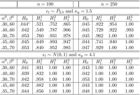
con-vergence. Standard and profile-weighted moment estimators are treated in Section 5, and are used for heavy tail robust (and efficient) score, Lagrange Multiplier, and Likelihood Ratio tests.
Such tests can be used as heavy tail robust model specification tests, including GARCH order or
the presence of GARCH effects, so they can be used as model selection tools.6 However, testing
when a parameter value is on the boundary of the maintained hypotheses leads to non-standard
asymptotics (Andrews, 2001).
In Section 3 we show that the implied probabilities derived from the tail-trimmed
Contin-uously Updated Estimator, which are especially tractable, differentiate between usable large
values (i.e. values near the trimming threshold) and damaging extremes that are trimmed for
estimation. Large values serve as leverage points and accelerate convergence rates, yet very large values impede normality and are therefore trimmed. Thus, extremes receive elevated weight, but
near-extremes that are not trimmed receive the most weight. We use the implied probabilities
from tail-trimmed GEL to perform heavy tail robust and efficient tests of over-identification.
Similar test statistics, without trimming, have been considered by Kitamura and Stutzer (1997),
Newey and Smith (2004), and Smith (2011) amongst others.
In Section 4 we derive a higher order expansion for our estimator along the lines of Newey
and Smith (2004, Sections 3 and 4). In the case of GARCH model estimation with QML-type
estimating equations, GEL requiresE[6
t]<∞ for a second order expansion (necessary for bias) andE[10
t ]<∞for a third order expansion, while GELITT always only needsE[2t]<∞for any higher order expansion. GELITT bias decomposes into bias due to the GEL structure (when
higher moments exist) and bias due to trimming. This is irrelevant for bias-correction since a
composite bias estimator as in Newey and Smith (2004, Section 5) removes higher order GELITT
bias whether due to the GEL form or trimming. Moreover, it does not require extreme value
theory and therefore tail index estimation as in Hill (2015b).
We also show that under mild assumptions (higher order) bias is always small if few
observa-tions are trimmed, and monotonically smaller in the case of EL or exact identification. By first
order asymptotics the rate of convergence is higher if the rate of trimming is nearly the sample
size n, a feature common to M-estimators for GARCH models with negligible trimming, and to
mean estimation, cf. Hill (2012, 2015b,a). Thus, trimming at a rate nearly equal to ζn, e.g.
ζn/ln(n), is optimal as long as a small ζ is used. The usefulness of this combination is revealed
by simulation in Section 8, and elsewhere (Aguilar and Hill, 2015; Hill, 2012, 2013, 2015b,a; Hill
and Aguilar, 2013). Together, the use of higher order asymptotics to minimize and estimate bias
marks a sharp improvement over existing tail-trimming methods for M-estimators (Hill, 2013,
2015b,a). In that literature, only first order asymptotics exist which, as in the present paper, invariably points toward elevating trimming by errors, but says little about the implications for
trimming on bias.
We then use the probability profiles in Section 6 for tail-trimmed moment estimation which
is shown to have the same efficiency property as without trimming. We generalized theory
developed in Smith (2011) for GEL estimators to the heavy tail case, while Smith (2011) extends
theory in Back and Brown (1993) and Brown and Newey (1998). As an example, in Section 7 we
use the profiles for efficient and heavy tail robust estimation of a conditionally heteroscedastic
asset’sexpected shortfall. We derive the limit distribution of a bias-corrected profile weighted
tail-trimmed estimator, making a more efficient version of Hill’s (2015b) robust estimator. Further, we improve on Hill’s (2015b) proposed strategy for optimally estimating bias, and derive the
appropriate limit theory.
GEL estimators (untrimmed or trimmed) have not been thoroughly studied for GARCH model
estimation.7 We use EL, CUE and ET criteria, with and without trimming, and for trimming we
use our higher order bias minimization theory for selecting the trimming fractile. Tail-trimmed
CUE performs best overall in terms of bias, mse, and approximate normality, evidently due to the easily solved quadratic criterion and the fact that trimming a few errors per sample improves
sampling properties. This is a useful result that may be of independent interest since EL with or
without trimming has lower higher order bias in theory. That theory, however, does not account
for substantial computational differences across GEL estimators, giving substantial credence to
the argument for simplicity in Bonnal and Renault (2004) and Antoine, Bonnal, and Renault
(2007). It also further demonstrates that trimming very few observations can have a strong
positive impact on estimator performance, as shown also in Hill (2013, 2015a).
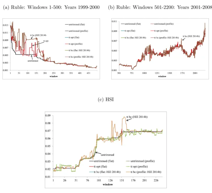
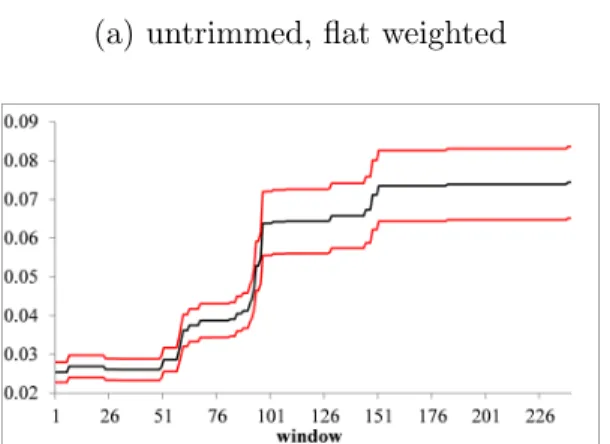
Finally, we perform a small scale empirical study based on financial returns in order to
demonstrate our GEL estimator, and our robust, efficient and bias-improved estimator of the expected shortfall. We leave concluding remarks for Section 10.
The theory of GEL to date is designed for sufficiently thin tailed equations such that
asymp-totic normality is assured. See Qin and Lawless (1994), Hansen, Heaton, and Yaron (1996),
Imbens (1997), Kitamura (1997), Kitamura and Stutzer (1997), Imbens, Spady, and Johnson
(1998), Smith (1997, 2011), Newey and Smith (2004), and Antoine, Bonnal, and Renault (2007)
for early contributions and broad theory developments. In a GARCH framework with
QML-type equations and only lags of st as instruments, we need E[4t] < ∞ (cf. Francq and Zako¨ıan, 2004), but a far more restrictive moment condition is needed if least squares-type equations are
used (see Francq and Zako¨ıan, 2000). Moreover, as discussed above, a higher order asymptotic
expansion for GEL estimators of GARCH models with QML-type equations require prohibitive moment conditions, up toE[10
t ]<∞for a third order expansion. Nevertheless, GEL estimators have beneficial properties: asymptotic bias of GEL does not grow with the number of estimating
equations, contrary to GMM in well known cases, while bias-corrected EL is higher order
asymp-totically efficient (see Newey and Smith, 2004; Anatolyev, 2005). The higher order properties
arise from different first order conditions for different GEL criteria, while first order asymptotics,
including efficiency, are insensitive to the criteria, whether there is weak identification or not
(cf. Newey and Smith, 2004; Guggenberger and Smith, 2008). We show that GELITT obtains
the same type of higher order expansion as GEL, without the requirement of higher moments.
Hence, the higher order bias and efficiency properties of GEL extend to GELITT under far less stringent conditions.
7Chan and Ling (2006) develope EL theory for AR-GARCH models, but only study a unit root test, and
Empirical likelihood for heavy tail robustness and for GARCH has limited use to date. Peng
(2004) uses the empirical likelihood method for heavy tail robust confidence bands of the mean,
and other than a similar use for tail parameter inference (Worms and Worms, 2011) there do
not appear to be any other extensions to robust estimation. Chan and Ling (2006) develop empirical likelihood for GARCH and random walk-GARCH, whereE[4
t]<∞ andα0 +β0 <1, both unrealistic restrictions for many financial time series. Further, they only study a unit root
test by simulation and therefore do not report GEL estimator properties for GARCH. Two-step
GMM estimation for GARCH is treated in Skoglund (2010), amongst others.
We use the following notation. TheLp-norm for a matrixA≡[Ai,j] is||A||p≡(
P
i,jE|Ai,j|p)1/p. The spectral norm is ||A||= (λmax(A0A))1/2 whereλmax is the maximum eigenvalue. K >0 is a
finite constant whose value may change; ι, δ > 0 are tiny constants; and N is a positive integer. p
→and→d denote convergence in probability and in distribution. →denotes convergence in|| · ||.
an ∼ bn implies an/bn → 1 as n → ∞. Id is a d-dimensional identity matrix. L(n) → ∞ is a slowly varying function whose value or rate may change from line to line. Anintermediate order
sequence {kn} satisfieskn ∈ {1, ..., n − 1}, andkn → ∞and kn/n → 0 as n → ∞.
2
GEL with Tail-Trimming
We initially work with the unobserved process {σ2
t(θ)} and derive an infeasible estimator of θ0. We then derive parallel results for the feasible estimator based on an iterated approximation to
σt2(θ). Drop θ0 throughout, e.g. σ2t = σ2t(θ0), xt =xt(θ0).
2.1
Tail-Trimmed Equations
Our first task is to trim the equations mi,t(θ) when they obtain an extreme value. Hill and Renault (2010) use mi,t(θ) itself to gauge when an extreme value occurs. Since mt may be asymmetric this requires asymmetric trimming which in general induces small sample bias. In
the present setting by a standard first order expansion we know asymptotics depend solely on
t(θ) and xt(θ). However, st(θ) = (∂/∂θ) lnσ2t(θ) has an L2-bounded envelope supθ∈N0|si,t(θ)|
on some compact subset N0 ⊆ Θ containingθ0 (cf. Francq and Zako¨ıan, 2004), hence only t(θ) and the added weights wt(θ) in xt(θ) can be sources of extremes in mt(θ). We therefore trim by these components separately.
Let zt(θ) denote t(θ) or wi,t(θ), and define the two-tailed process and its order statistics:
zt(a)(θ)≡ |zt(θ)| and z
(a)
(1)(θ)≥ · · · ≥z (a)
Let {kn(), ki,n(w)} for i ∈ {1, ..., q − 3} be intermediate order sequences. We use intermediate order statistics(a)
(kn())
(θ) andw(a)
i,(k(i,nw))(θ) to gauge when an extreme observation occurs, a common
practice in the extreme value theory and robust estimation literatures. See Hill (2011) for
references. Now define indicator functions for trimming
ˆ
In,t()(θ)≡I|t(θ)| ≤
(a) (k(n))
(θ)
ˆ
Ii,n,t(w)(θ)≡I
|wi,t(θ)| ≤w
(a)
i,(k(i,nw))(θ)
and ˆIn,t(x)(θ)≡
q−3
Y
i=1
ˆ
Ii,n,t(w)(θ) if q >3
1 if q = 3,
and tail-trimmed variables and equations
ˆ
∗n,t(θ)≡t(θ) ˆI
()
n,t(θ) and ˆw
∗
n,t(θ)≡wt(θ) ˆI
(w)
n,t(θ) and ˆx
∗
n,t(θ)≡
st(θ)0,wˆ∗n,t(θ)
0
ˆ
m∗n,t(θ)≡ ˆ∗n,t2(θ)− 1 n
n
X
t=1
ˆ
∗n,t2(θ)
!
×xˆ∗n,t(θ). (3)
As in Hill (2015a) and Aguilar and Hill (2015), we re-centert(θ) after trimming to eradicate small sample bias that arises from trimming. This allows for intrinsically simpler symmetric
trimming even if t has an asymmetric distribution.
If over-identifying restrictions are not used such that xt(θ) = st(θ), then we use
ˆ
m∗n,t(θ)≡ ˆ∗n,t2(θ)− 1 n
n
X
t=1
ˆ
∗n,t2(θ)
!
×st(θ) where ˆ∗n,t(θ)≡t(θ) ˆI
()
n,t(θ).
If any added instrumentwi,t has a finite variance then we do not need to trim by it. It is easy to show, however, that if we trim by all components inwt(θ) then it is asymptotically equivalent to only trimming by those elements with an infinite variance (cf. Hill, 2015a, 2013). We therefore
assume that each wi,t(θ) is trimmed in order to reduce notation.
Although st(θ) has an L2-bounded envelope, in small samples components of st(θ) may be influenced by large observationsyt−1. Consider that in the case of no GARCH effectsα0 +β0 =
0, it followsst= (ω0)−1×[1, yt2−1, ω0]0. Thus, in view of continuity, ifα0+β0 is close to zero then ||st||may be large whenyt−1 is large. Although Gaussian asymptotics does not require trimming
yt−1 for trimming, even when α0 +β0 is far from zero. In this case the trimmed covariates are
ˆ
x∗n,t(θ)≡
ˆ
s∗n,t(θ)0,wˆ∗n,t(θ)0 where ˆs∗n,t(θ)≡st(θ) ˆI
(y)
n,t−1 and ˆI (y)
n,t−1 ≡I
|yt| ≤y
(a) (kn(y))
. (4)
Since the asymptotic theory for our GEL estimator with ˆx∗n,t(θ) defined as [st(θ)0, wˆ∗n,t(θ)
0]0 or
[ˆs∗n,t(θ)0, wˆ∗n,t(θ)0]0 is the same, we simply assume the former to reduce notation in the proofs.
2.2
Estimator
Letρ:D →R+be a twice continuously differentiable concave function, with domainDcontaining
zero. Write ρ(i)(u) = (∂/∂u)iρ(u),i = 0,1,2, and ρ(i) = ρ(i)(0), and assume the normalizations ρ(0) = ρ(0) = 0 andρ(1) = ρ(2) = −1. If ρ(u) = −u2/2− u we have the Continuously Updated
Estimator or Euclidean Empirical Likelihood (cf. Antoine, Bonnal, and Renault, 2007); ρ(u) =
ln(1 − u) for u < 1 leads to Empirical Likelihood; ρ(u) = 1 − exp{u} represents Exponential Tilting.
The GEL estimator with Imbedded Tail-Trimming (GELITT) solves a classic saddle-point
optimization problem (Smith, 1997; Newey and Smith, 2004; Smith, 2011):
ˆ
θn= arg min θ∈Θ
sup λ∈Λˆn(θ)
(
1
n
n
X
t=1
ρ λ0mˆ∗n,t(θ)
)
and ˆλn = arg sup λ∈Λˆn(ˆθn)
(
1
n
n
X
t=1
ρλ0mˆ∗n,t(ˆθn)
)
, (5)
where ˆΛn(θ) contains thoseλ such that sample λ0mˆ∗n,t(θ)∈ D with probability one:
ˆ Λn(θ) =
λ:λ0mˆ∗n,t(θ)∈ D a.s., t= 1,2, ..., n .
The non-smoothness of ˆm∗n,t(θ) is irrelevant as long as wi,t(θ) are differentiable, and t(θ) and
wi,t(θ) have smooth distributions (Parente and Smith, 2011; Hill, 2015a, 2013).
Asymptotics for [ˆθn0,ˆλ0n]0 requires non-random threshold sequences associated with the sample order statistics. Let positive sequences of functions {c(n)(θ), ci,n(w)(θ),} satisfy for any θ ∈ Θ
P |t(θ)| ≥c(n)(θ)
= k
()
n
n and P
|wi,t(θ)| ≥c
(w)
i,n(θ)
= k
(w)
i,n
n . (6)
Thus, for example, (a) (k(n))
(θ) estimates c(n)(θ) since (a)
(kn())
trimming indicator functions
In,t()(θ)≡I |t(θ)| ≤c(n)(θ)
and Ii,n,t(w)(θ)≡I|wi,t(θ)| ≤c
(w)
i,n(θ)
,
write the composite covariate indicatorIn,t(x)(θ) = Qq−3
i=1 I (w)
i,n,t(θ), and define tail-trimmed variables and equations
∗n,t(θ)≡t(θ)In,t()(θ) and w
∗
n,t(θ)≡wt(θ)In,t(w)(θ)
mn,t∗ (θ)≡ n,t∗2(θ)−E
∗n,t2(θ)
x∗n,t(θ)−E
x∗n,t(θ)
.
In view of the re-centering of t(θ) for ˆm∗n,t(θ) in (3), it can be shown that asymptotics for ˆθn are grounded on m∗n,t(θ). See the appendix.
Notice by error independence, re-centering, and =t−1-measurability of xt, it follows m∗n,t is a martingale difference with respect to =t since
E
m∗n,t|=t−1
= x∗n,t−E
x∗n,t
×E
∗n,t2 −E
∗n,t2
)
|=t−1
= 0. (7)
2.3
Main Results
Define moment suprema for t(θ), and wi,t(θ) provided over-identifying weights are used:
κ(θ)≡sup{α >0 :E|t(θ)|α <∞} and κi(θ)≡sup{α >0 :E|wi,t(θ)|α <∞}.
Note that κ =∞orκi =∞are possible, for example if t is Gaussian, orwi,t is bounded.8 Let Θ1,i ⊆ Θ be the set of allθ such that κi(θ) ≤1, where Θ1,i may be empty. Dropθ0 such that κ = κ(θ0) and κi = κi(θ0).
We require the following moment, memory and tail properties.
Assumption A.
1. zt(θ)∈ {t(θ), wi,t(θ)}have for each θ ∈Θstrictly stationary, ergodic, and absolutely
continu-ous non-degenerate finite dimensional distributions that are uniformly bounded: supa∈R,θ∈Θ{(∂/∂a)P(zt(θ)
≤ a)} < ∞ and supa∈R,θ∈Θ||(∂/∂θ)P(zt(θ) ≤ a)|| < ∞.
2. κi >1and κ >2. If κ ≤ 4then P(|t|> a) =da−κ(1 +o(1)) where d ∈(0,∞). If Θ1,i is
8Consider an ARCH(1) model σ2
t =ω0 +α0yt2−1 with ω0, α0 >0. Then, for example, the weights xt(θ) =
not empty such that κi(θ)≤ 1 for some θ, then P(|wi,t(θ)| > c)} =di(θ)c−κi(θ)(1 +o(1)) where infθ∈Θ1,idi(θ) >0, infθ∈Θ1,iκi(θ)> 0 and o(1) is not a function of θ.
3. wt(θ) is =t−1-measurable, continuous, differentiable, and E[supθ∈Θ|wi,t(θ)|ι] < ∞ for some
tiny ι > 0.
4. kn/nι → ∞for some tiny ι > 0.
Remark 1 Distribution continuity and differentiability of mt(θ) = (2t(θ) − 1)xt(θ) ensure a
unique solution to the GELITT estimation problem exists (cf. Cizek, 2008; Hill, 2015a, 2013).
Remark 2 Paretian tails in the heavy tail case simplify characterizing tail-trimmed moments by
Karamata’s Theorem, while tail-trimmed moments arise in the GELITT estimator scale, defined
below. We impose a Paretian tail on wi,t(θ) when κi(θ) ≤ 1 since the mapping wi,t : Θ→ R is not here defined. If the mapping were known then in principle we would only need to consider
wi,t.
Remark 3 We impose a lower bound on how fast the number of trimmed extremeskn increases
in order to simplify proving a uniform law of large numbers for tail-trimmed dependent data.
See Lemma A.4 in the appendix, and its proof in Hill and Prokhorov (2014).
Remark 4 If wt(θ) only contains lags of st(θ) then supθ∈Θ||wt(θ)|| is L2-bounded in view of α
+ β > 0 (Francq and Zako¨ıan, 2004), hence Θ1,i is empty and A.3 holds.
We now state the main results. Let 0 be a q × 1 vector of zeros. Define all parameters
ϑ0 ≡[θ00,00]0 ∈Rq+3 and ˆϑ
n ≡[ˆθ0n,λˆ
0
n]
0 ∈
Rq+3,
and define covariance and scale matrices
Σn(θ)≡E
m∗n,t(θ)m∗n,t(θ)0∈Rq×q (8)
Jn(θ)≡ −E
x∗n,t(θ)−Ex∗n,t(θ)(st(θ)−E[st(θ)])
0
∈Rq×3
Vn(θ)≡nJn(θ)0Σn−1(θ)Jn(θ)∈R3×3
An ≡
"
Vn 0 0 nP−1
n
#
∈R(q+3)×(q+3) where Pn≡Σ−n1−Σ
−1
n Jn Jn0Σ
−1
n Jn
−1
The mean-centered Jacobian Jn arises from the re-centered error in the estimating equations ˆ
m∗n,t(θ) = (ˆn,t∗2(θ)−1/nPn
t=1ˆ
∗2
n,t(θ))×xˆ∗n,t(θ),since this is asymptotically equivalent tom∗n,t(θ) = (∗n,t2(θ) − E∗n,t2(θ))) × (x∗n,t(θ)− Ex∗n,t(θ)).
We first prove consistency from first principles, since a standard first order expansion for asymptotic normality involves an estimator ofJn. We can only analyze the latter asymptotically if we first know ˆθn
p
→ θ0. See Appendix A for all proofs.
Theorem 2.1 Under Assumption A θˆn
p
→ θ0 and n1/2Σ1/2
n λˆn = Op(1).
Second, ˆθn and ˆλn are jointly asymptotically normal.
Theorem 2.2 Under Assumption A A1n/2( ˆϑn − ϑ0)
d
→ N(0, Iq+3), in particular V 1/2
n (ˆθn − θ0) d
→ N(0, I3).
Remark 5 The GELITT scalesAnandVnare identical in form to the scales for the conventional
GEL estimator (Newey and Smith, 2004).
Remark 6 By the martingale difference property, E[2
t] = 1 and dominated convergence, it follows
Σn = E
h
∗n,t2 −E
∗n,t22i
×Eh x∗n,t−E
x∗n,t
x∗n,t−E
x∗n,t0i
∼ E∗n,t4−1×Eh x∗n,t−Ex∗n,t x∗n,t−Ex∗n,t0i.
Hence, in the case of exact identificationxt(θ) = st(θ) we have Jn =E[(st −E[st])(st −E[st])0] and therefore
Vn ∼n 1
E
∗4
n,t
−1E
(st−E[st]) (st−E[st])
0
.
Similarly, when xt(θ) contains only st(θ) and its lags then
kVnk ∼Kn 1
E∗4
n,t
.
The same order applies whenever xt is square integrable, e.g. it only containsst and its lags. In this case if Xt ≡ xt − E[xt] and St ≡ st − E[st] then:
Vn ∼n 1
E∗4
n,t
−1V where V =J
0
Σx−1J,J =−E[XtSt0] and Σx =E[XtXt0].
Hence (n/(E[∗4
n,t]− 1))1/2(ˆθn − θ0) d
Remark 7 IfE[4
t]<∞andxtis square integrable then GELITT obtains the same asymptotic distribution as the untrimmed GEL estimator: n1/2(ˆθn − θ0)
d
→ N(0,(E[t4]−1)V−1), with V
defined above.
Remark 8 Notice
nPn−1 =nΣn
I− Jn Jn0Σ
−1
n Jn
−1
Jn0Σ−n1
−1
∼KnΣn
hence ˆλn has a faster rate of convergence than ˆθn when E[4t] = ∞. Indeed, by Theorem 2.1 the rate is n1/2||Σ
n||1/2 ∼ Kn1/2E[∗n,t4]× ||E[x
∗
n,tx
∗0
n,t]|| which is greater thann1/2 when E[4t] = ∞.
The rate of convergence can be easily obtained if over-identifying weights wt are square integrable, e.g. wtonly contain lags of the scorest, since thenxtisL2-bounded and the Jacobian Jn = −E[(x∗n,t − E[x∗n,t])(st−E[st])0] is uniformly bounded: lim supn→∞||Jn|| ≤ K. In order to see this, by construction of the thresholds and power law Assumption A.2, if κ ∈ (2,4] then
c(n) = d1/κ(n/kn())1/κ. Therefore if E[4t] =∞then by Karamata’s Theorem9
κ ∈(2,4) : E
∗n,t4 ∼ 4
4−κ
c(n)4P |t|> c(n)
= 4 4−κ
d4/κ
n
kn()
4/κ−1
(9)
κ = 4 :E
∗n,t4 ∼dln(n).
In either case κ = 4 orκ ∈ (2,4) it follows
E∗n,t4−1 =E∗n,t4×(1 +o(1)). (10)
Combine Theorem 2.2 with (9) and (10) to deduce the next result.
Corollary 2.3 Let Assumption A hold, and if q > 3 then let wt be square integrable. Then
κ ∈(2,4) :
n1/2
n/kn()
2/κ−1/2
ˆ
θn−θ0
d
→ N
0, 4
4−κ
d4/κ× V−1
κ = 4 :
n
ln(n)
1/2
ˆ
θn−θ0
d
→ N 0, d× V−1
9See Theorem 0.6 in Resnick (1987). The caseκ
= 4 follows by observing ifκ= 4 thenc
()
n =d1/4(n/kn())1/4,
hence for finitea >0 there existsK >0 such thatE[4
tI
()
n,t] =
R(c(n))4
0 P(|t| > u
1/4)du =K +R(c(n))4
a u
−1du =
where V ≡ J0Σ−1
x J with J ≡ −E[(xt − E[xt])(st − E[st])0] and Σx ≡ E[(xt − E[Xt])(xt −
E[xt])0].
As long as t has an unbounded fourth momentκ ∈(2,4], the rate of convergence is o(n1/2). Ifκ ∈(2,4) then by maximizing the trimming amountk
()
n and therefore makingkn() arbitrarily close to a fixed portionζnofnwhereζ ∈(0,1), we can optimize the rate of convergence. Simply
letk(n) ∼n/gn for gn→ ∞ at a slow rate to deduce ˆθn can be made as close ton1/2-convergent as we choose. A parametric rule for k(n) is convenient, for example
kn() = [ζn/ln (n)] where ζ ∈(0,1]. (11)
Then for any κ ∈ (2,4) we have
n1/2
(ln (n))2/κ−1/2
ˆ
θn−θ0
d
→ N(0,V(ζ, κ, d)), with V(ζ, κ, d)≡ 1
ζ4/κ−1
4 4−κ
d4/κ× V−1.
(12)
In this case the rate of convergence is identical to Quasi-Maximum Tail-Trimmed Likelihood
in Hill (2015a) since the estimating equations are identical or similar to QML score equations.
Thus, whenκ ∈(2,4] the GELITT estimator converges faster than QML as long ask(n) ∼n/gn for slow gn → ∞ (see Hill, 2015a).
Notice that by letting ζ be large we can diminish the asymptotic variance V(ζ, κ, d). By first order asymptotics, it is always better to trim more extreme values per sample since we
achieve both a higher rate of convergence and lower asymptotic variance. However, in Section 4
we exploit higher order asymptotics and show that the higher order bias of GELITT is smaller
when trimming is reduced.10 In the case of EL or exact identification, the bias monotonically
decreases as trimming is reduced. Indeed, it is easily revealed by simulation that a greater
amount of trimming induces small sample bias for standard GEL criterion, e.g. EL, CUE, and
ET. Thus, while first order efficiency and the rate of convergence are augmented with a trimming
rule like (11) with largeζ, higher order bias is reduced by setting ζ small, e.g. ζ = .05 as we do in the Section 8 simulation study.
In principle, there is an optimal trimming rule implied by the combination of the first and
higher order asymptotic arguments. However, a higher order mean-squared-error will favor
efficiency in heavy tailed cases since the higher order variance will dominate the squared bias.
Minimizing this mean-squared-error is not practical since it will simply lead to setting kn() close
10We thank a referee for suggesting that second order asymptotics can be useful in justifying optimal trimming
ton. Nevertheless, the preceding points to a dominant strategy: elevate the rate of convergence
while controlling higher order bias by elevating the rate k(n) → ∞ as n → ∞ and, for a given sample, by setting k(n) as a small value relative ton.
Finally, although the GELITT rate is optimized to its upper boundn1/2 whenk(n)= [ζn], we cannot use a fixed portion since ˆθn need not be consistent forθ0. This follows since 1/nPnt=1ˆ∗n,t2
p
→[0,1) under Assumption A, hence the centered error ˆ∗2
n,t(θ)−1/n
Pn
t=1ˆ
∗2
n,t(θ) in ˆm
∗
n,t(θ) may not identifyθ0 (see, e.g., Sakata and White, 1998; Mancini, Ronchetti, and Trojani, 2005). If the
distribution of t were assumed, this bias can in theory be removed by simulation-based indirect inference, as in Cantoni and Ronchetti (2001) and Ronchetti and Trojani (2001).
2.4
Feasible GELITT
In practice σ2
t(θ) cannot be computed for t ≤ 1, so an iterated approximation must be used. Define
ht(θ) = ˜ω >0 for t= 0, and ht(θ) = ω+αyt2−1+βht−1(θ) for t= 1,2, ... (13)
where ˜ωis not necessarily an element ofθ0. Writehθt(θ)≡(∂/∂θ)ht(θ) andh θ,θ
t (θ)≡(∂/∂θ)hθt(θ). Under Assumption A it can be shown that stationary and ergodic solutions to (13) and the corresponding equations forhθ
t(θ) andh θ,θ
t (θ) exist (see Lemma A.7 in Hill, 2014a, cf. Meitz and Saikkonen, 2011).
Now replace σ2
t(θ) with ht(θ) and define
˚t(θ)≡
yt
ht(θ)1/2
and ˚st(θ)≡ 1
ht(θ)
hθi,t(θ) and ˚xt(θ)≡[˚st(θ)0,w˚t(θ)0]
0
.
We write ˚wt(θ since the added instruments may be a function of ht(θ), for example when ˚wt(θ) contains lags of ˚st(θ). The tail-trimmed versions are
b
˚∗n,t(θ)≡˚t(θ)I
|˚t(θ)| ≤˚
(a) (k(n))
(θ) and ˚bx
∗
n,t(θ)≡
h
˚st(θ)0,wb˚
∗
n,t(θ)
0i0
˚∗n,t(θ)≡˚t(θ)I |˚t(θ)| ≤c(n)(θ)
and ˚x∗n,t(θ)≡
˚st(θ)0,w˚n,t∗ (θ)
0
,
hence the equations are
b
˚
m∗i,n,t(θ)≡ b˚
∗
n,t(θ)− 1
n
n
X
t=1
b
˚∗n,t(θ)
! b
˚
m∗i,n,t(θ)≡ ˚∗n,t(θ)−E˚∗n,t(θ) ˚x∗n,t(θ)−E˚x∗n,t(θ),
and the feasible estimators are
b
˚θ
n= arg min θ∈Θ
sup λ∈Λˆn(θ)
(
1
n
n
X
t=1
ρλ0m˚b
∗
n,t(θ)
)
and˚bλ
n= arg sup λ∈Λˆn(˚bθ
n)
(
1
n
n
X
t=1 ρ
λ0m˚b
∗
n,t(b˚θn)
)
.
Define b˚ϑ
n ≡ [˚bθ
0
n,˚bλ
0
n]
0. The feasible and infeasible estimators have the same limit distribution.
The proof is similar to the proof of Theorem 2.3 in Hill (2015a) and is therefore omitted.
Lemma 2.4 Under Assumption A A1n/2(ϑ˚bn−ϑˆn) p
→0.
We only work with the infeasible ˆϑn in all that follows for the sake of notational ease.
3
Extremal Information of Implied Probabilities
Recallρ(1)(u) = (∂/∂u)ρ(u). By the GELITT first order condition it is easy to show the implied
probabilities or profiles have a classic form (Antoine, Bonnal, and Renault, 2007; Newey and
Smith, 2004)
ˆ
πn,t∗ (θ) =
ρ(1)
ˆ
λ0nmˆ∗n,t(θ)
Pn
t=1ρ(1)
ˆ
λ0
nmˆ∗n,t(θ)
where ˆλn = arg sup
λ∈Λˆn(ˆθn)
(
1
n
n
X
t=1
ρλ0mˆ∗n,t(ˆθn)
)
. (14)
See Appendix A.3 for derivation of the first order condition, equation (A.8). The profiles ˆπn,t∗ (θ) promote an empirical counterpart to the GELITT identification condition E[m∗n,t(θ0)] = 0 since ˆ
πn,t∗ (θ) ∈ [0,1],Pn
t=1πˆ
∗
n,t(θ) = 1, and by the first order condition
Pn
t=1πˆ
∗
n,t(θ) ˆm∗n,t(ˆθn) = 0. We begin by gleaning information about extremes from ˆπn,t∗ (θ) in the case of tail-trimmed CUE due to its tractability. Since ρ is quadratic in this case we have (Antoine, Bonnal, and
Renault, 2007)
ˆ
πn,t∗ (θ) = 1 + ˆλ
0
nmˆ
∗
n,t(θ)
Pn
t=1
n
1 + ˆλ0
nmˆ∗n,t(θ)
o. (15)
Now define the set of time indices at which an error is trimmed:
b
In∗(θ)≡
Thus, since ˆ∗n,t(θ) ≡ t(θ) ˆI
()
n,t(θ)
Qq−3
i=1 Iˆ (w)
i,n,t(θ), then t ∈ Ibn∗(θ) when t is large, or any
over-identifying weightwi,t(θ) is large. Then for anyt∈Ibn∗(θ) we have ˆm∗n,t(θ) =−(1/n Pn
s=1ˆ
∗2
n,s(θ))
× xˆ∗n,t(θ) a.s., hence by dominated convergence and limit theory developed in the appendix:
ˆ
m∗n,t(θ) = −xˆn,t∗ (θ)×(1 +op(1)). (16)
By imitating arguments in Antoine, Bonnal, and Renault (2007, Theorem 3.1),ˆπ∗n,t(θ) has the decomposition
ˆ
πn,t∗ (θ) = 1
n −
1
nmˆ
∗
n(θ)
0ˇ
Σ−n1(θ)×
ˆ
m∗n,t(θ)−mˆ∗n(θ) (17)
where
ˆ
m∗n(θ)≡ 1 n
n
X
t=1
ˆ
m∗n,t(θ) and ˇΣn(θ)≡ 1 n n X t=1 ˆ
m∗n,t(θ)−mˆ∗n(θ) mˆ∗n,t(θ)0.
Since ˆm∗nΣˇ−n1mˆ∗n > 0a.s. and ˆm∗n →p 0, it follows by (16) and (17) that periods with a trimmed error have an elevated profile ˆπn,t∗ :
ˆ
πn,t∗ = 1
n +
1
nmˆ
∗
n
0ˇ
Σ−n1mˆ∗n+ 1
nmˆ
∗
n
0ˇ
Σ−n1xˆ∗n,t×(1 +op(1)) = 1
n +
1
nmˆ
∗
n
0ˇ
Σ−n1mˆ∗n(1 +op(1))> 1
n a.s.
Lemma 3.1 We have πˆn,t∗ > 1/n with probability approaching one for each period t with a
trimmed error (due to a large error and/or large over-identifying weight).
We can go further by applying limit theory presented in the appendix to (17) to obtain
ˆ
π∗n,t = 1
n +
1
n2
(
1
n1/2Σ
−1/2
n n
X
t=1
ˆ
m∗n,t
)0(
1
n1/2Σ
−1/2
n n
X
t=1
ˆ
m∗n,t
)
(1 +op(1))
= 1
n +
1
n2 × X 2
q ×(1 +op(1)) = 1
n
1 + 1
n × X 2
q ×(1 +op(1))
where t ∈ Ibn∗, where Xq2 is a chi-squared random variable with q degrees of freedom. Since
such ˆπ∗n,t satisfy n2(ˆπ∗
n,t − 1/n) d
→ X2
q and ˆπ
∗
n,t = n
−1 + n−2X2
q(1 + op(1)) ∈ [0,1], apply the Helly-Bray Theorem to deduce on average ˆπn,t∗ is 1/n+ q/n2 + o
p(1/n2) in periods in which an extreme error occurs.
Lemma 3.2 E[ˆπn,t∗ | t ∈ Ibn∗] = 1/n +q/n2+op(1/n2)).
Although periods with extremes are deemed damaging for asymptotics, this does not imply
value 1/n. Rather, tail-trimmed CUE assigns periods with exceptionally large errors or weights
anelevated (relative to uniform 1/n) probability, roughly on average 1/n + q/n2 for large n.
But this begs the question regarding which periods are being assigned smaller or larger profiles
in general. Decomposition (17) and limit theory in the appendix reveal in any period t
ˆ
πn,t∗ = 1
n
1 + 1
nX 2
q (1 +op(1))
− 1 n
(
1
n1/2Σ
−1/2
n n
X
t=1
ˆ
m∗n,t
)0
× 1 n1/2Σ
−1/2
n mˆ
∗
n,t(1 +op(1))
= 1
n
1 + 1
nX 2
q − Z
0× 1
n1/2Σ
−1/2
n mˆ
∗
n,t
(1 +op(1)),
where Z is a standard normal random variable on Rq that satisfies identicallyX2
q =Z0Z. Now assume n is sufficiently large that 1/nPn
t=1ˆ
∗2
n,t ≈1 hence ˆm∗n,t ≈(ˆn,t∗2 − 1)ˆx∗n,t2.
An asymptotic random draw {yt}∞t=1 with a propensity for large errors t and therefore large ˆ
mn,t∗ > 0 implies a larger likelihood that Z0 ×Σn−1/2mˆ∗n,t > 0. But this implies ˆπ
∗
n,t < n
−1{1 +
n−1X2
q}for many periodstwhen a large error occurs. Thus, in an asymptotic draw when a large error is not particularly rare then any given t with a large error is not especially informative:
the ascribed profile weight is closer to the flat weighted value n−1 than in periods of extreme
values. Put differently, a periodt that “goes with the flow” is not particularly useful for efficient
moment estimation by profiling weighting. In fact, in a sample with many large t, any period with a very large t that is not so large as to be trimmed is, in probability, the least useful in the sense of receiving the smallest ˆπ∗n,t.
Contrariwise, periods that go “against the flow,” that is, periods when ˆm∗n,t <0, are assigned the largest ˆπn,t∗ . This arises either when t is small and wi,t are not extreme values such that ˆ
∗2
n,t <1, or t and/or wi,t are so large that t is trimmed hence ˆm∗n,t ≈ − xˆ
∗2
n,t. Intuitively, large values are useful only if they portray dispersion or leverage: a large ˆm∗n,t > 0 amongst many large positive ˆm∗n,t does not provide much useful information. See also Back and Brown (1993) for a classic interpretation of ˆπn,t∗ .
4
Higher Order Asymptotics and Fractile Choice
In Appendix A.3 we derive the first order expansion:
A1/2
n
ˆ
ϑn−ϑ0
=−InΣ−n1/2 1
n1/2
n
X
t=1
where In ∈ R3×q satisfies In0In = I3. The expansion with op(1) replaced with 0 is identical to the GEL first order expansion in Newey and Smith (2004, eq. (A.8)). Since m∗n,t is a martingale difference with E[m∗n,tm∗0n,t] = Σn for any fractile sequences {k
()
n , ki,n(w)}, expansion (18) is not helpful for understanding how kn() influences small bias. Further, in terms of efficiency for the GARCH parameter estimator ˆθn, a choice ofk
()
n nearly equal toζnforζ ∈(0,1) will minimizeVn by Corollary 2.3. Thus, by first order asymptotics the best guidance we have is to usek(n) ∼n/gn for essentially any slowly increasing gn → ∞, e.g. k
()
n = [ζn/ln(n)]. In this case Corollary 2.3 shows that larger ζ is associated with a lower asymptotic variance. In simulation experiments,
however, it is easily seen that a small ζ leads to sharp inference since only then is the small
sample bias reduced.
We now shed some light on bias by formally deriving a higher order expansion and use higher
order bias to gauge what an optimal number of trimmed observations kn() should be. We also propose a bias-corrected estimator that corrects for bias due to the GEL structure and due to tail-trimming.
In order to reduce the number of trimming fractiles considered, and without affecting the
applicability of our derivations, assume over-identifying instruments wt are square integrable (e.g. xt contains only lags of st) and therefore need not be trimmed:
mn,t∗ (θ)≡ n,t∗2(θ)−E
∗n,t2(θ)
(xt(θ)−E[xt(θ)]) where ∗n,t(θ)≡t(θ)I
()
n,t(θ).
Allowing for trimming on the error and instruments would substantially complicate the
ex-pansion, but the salient features of our analysis below would still carry over: trimming few
observations promotes smaller higher order bias.
4.1
Higher Order Expansion
Similar to (18), we need only look to arguments in Newey and Smith (2004) to obtain a higher
order expansion. Let {z∗
n,t} be a tail-trimmed random variable. In order to express an asymp-totically valid derivative of a tail-trimmed object, let zn,t∗ (θ)≡ zt(θ)In,t(θ) where zt(θ) is differ-entiable, In,t(θ)∈ {0,1} and infθ∈ΘIn,t(θ)
p
→1, and define11
˚
∂
˚
∂θz
∗
n,t(θ)≡
∂ ∂θzt(θ)
×In,t(θ).
11The asymptotic theory supporting the use of such a derivative can be found in the appendices Hill (2013,
Define
M∗n,t(ϑ)≡ρ(1) λ0m∗n,t(θ)×
˚ ∂ ˚ ∂θm ∗
n,t(θ)
0λ
m∗n,t(θ)
G∗n(ϑ)≡E
" ˚ ∂ ˚ ∂ϑM ∗
n,t(ϑ)
#
, G∗j,n(ϑ)≡E
"
˚
∂2
˚
∂ϑj˚∂ϑ
M∗n,t(ϑ)
#
, G∗j,k,n(ϑ)≡E
"
˚
∂3
˚
∂ϑj˚∂ϑk˚∂ϑ
M∗n,t(ϑ)
#
A∗n,t≡ ˚∂
˚
∂ϑM
∗
n,t−G
∗
n and ψ
∗
n,t≡ −G
∗−1
n M
∗
n,t.
Since arguments merely mimic the proof of Lemma A.4 and Theorem 3.1 in Newey and Smith
(2004), we prove the following claim in Hill and Prokhorov (2014). Write ˜zn ≡1/n1/2Pnt=1zn,t∗ .
Theorem 4.1 Under Assumption A and ||E[wtw0t]|| < ∞:
ˆ
ϑn−ϑ0 = 1
n1/2ψ˜
∗
n+ 1
nQ1
˜
ψ∗n+ 1
n3/2Q2
˜
ψ∗n+Op
E∗4
n,t
2
n2
!
, (19)
where Q1( ˜ψ∗n) ≡ −Gn∗−1{Ae∗nψ˜∗n + 1/2 Pq+3
i=1 ψ˜
∗
i,nG∗i,nψ˜n∗} and Q2( ˜ψn∗)≡ −G∗−n 1Qn, with
Qn=Ae∗nQ1
˜
ψn∗+1 2 q+3 X i=1 n ˜
ψ∗i,nG∗i,nQ1( ˜ψn∗) +Qi,1( ˜ψ∗n)G
∗
i,nψ˜
∗
n+ ˜ψ
∗
i,nG
∗
i,nψ˜
∗ n o +1 6 q+3 X i,j=1 ˜
ψi,n∗ ψ˜j,n∗ G∗i,j,nψ˜∗n.
If k(n) ∼ n/L(n) for some slowly varying L(n) → ∞ then for any κ > 2:
ˆ
ϑn−ϑ0 = 1
n1/2ψ˜
∗
n+ 1
nQ1
˜
ψ∗n+Op
L(n)
n3/2
for slowly varying L(n)→ ∞ (20)
hence the asymptotic (higher order) bias for any κ > 2 is Bias( ˆϑn) = n−1E[Q1( ˜ψn∗)].
Remark 9 Since ˜ψ∗n is a function of ∗2
n,t and Ae∗n is a function of ∗n,t4, it is easily verified that
||E[Q1( ˜ψn∗)]|| ∼ KE[
∗6
n,t] and ||E[Q2( ˜ψn∗)]|| ∼ KE[
∗10
n,t]. If we were to disband with trimming and use a third order expansion as above, then we need E[10
t ] < ∞ just to deduce E[Q1]
represents asymptotic (higher order) bias, cf. Rothenberg (1984) and Newey and Smith (2004).
The analysis in Newey and Smith (2004) of higher order GEL properties, like bias and efficiency,
expansion with a remainder: using only a second order expansion reduces the higher moment
burden for GEL toE[6t]<∞. Negligible tail-trimming, however, allows us to impose onlyE[2t]
< ∞and still retain the same structure of higher order terms for GELITT.
Remark 10 The higher order terms are complicated by tail trimming. Notice ˆϑn exhibits two
forms of dynamics: one due to the GEL structure itself, and one due to trimming:
ˆ
ϑn−ϑ0 =
1
n1/2ψ˜n+
1
nQ1
˜
ψn
+ 1
n3/2Q2
˜
ψn
+Op
E
∗4
n,t
2
n2
!
+ 1
n1/2
˜
ψn∗ −ψ˜n
+ 1
n
Q1
˜
ψn∗−Q1
˜
ψn
+ 1
n3/2
Q2
˜
ψn∗−Q2
˜
ψn
,
where terms without ”∗” do not have trimming. Notice {·} contains GEL higher order terms
(Newey and Smith, 2004, Theorem 3.4), and the remaining terms describe the impact of
trim-ming. Thus if E[10
t ]< ∞then the GELITT (higher order) bias isE[Q1( ˜ψn∗)]/n =E[Q1( ˜ψn)]/n + {E[Q1( ˜ψ∗n)] − E[Q1( ˜ψn)]}/n, hence
Bias(GELIT T) = Bias(GEL) + Bias(trimming).
Remark 11 Result (20) shows n−1E[Q
1( ˜ψn∗)] expresses higher order bias when k
()
n ∼ n/L(n) for slowly varyingL(n)→ ∞, ultimately due to Karamata theory. Recall that such a trimming
rate optimizes the rate of convergence.
4.2
Higher Order Bias and Fractile Choice
In principle a higher order mean-squared-error can be computed and this can be minimized,
or at least inspected, in order to select the trimming fractile. We focus on bias n−1E[Q 1( ˜ψn∗)] in order to conserve space since the (higher order) variance is a tedious function of trimmed
moments, even if only based on n−1/2ψ˜n∗ + n−1Q1( ˜ψn∗). See also Newey and Smith (2004, p. 234). Nevertheless, bias reveals salient features that will carry over to (higher order) mean-squared-error computation.
Recall the criterion function notationρ(i)(u) = (∂/∂u)iρ(u), and now assumeρ(3)(u) exists, as
it does for EL, CUE and ET. Independence of the errors implies thatE[Q1( ˜ψn∗)] for GELITT has the same form asE[Q1( ˜ψn)] for GEL. The proof of the following result closely follows arguments in Newey and Smith (2004, proof of Theorem 4.2), and otherwise uses easily derived forms for
tail-trimmed GEL components for GARCH model estimation. See Hill and Prokhorov (2014)
Theorem 4.2 Write Xt ≡ xt − E[xt] and St ≡ st − E[st], and define E
(1)
n ≡ E[∗n,t2], En(i) ≡
E[(∗2
n,t − E
∗2
n,t
)i] for i = 2,3, J = −E[X0
tSt], Σx ≡ E[XtXt0], H ≡ (J
0Σ−1
x J)
−1J0Σ−1
x ∈
R3×q, P ≡ Σ−x1 − Σx−1J(J0Σ−x1J)
−1 J0Σ−1
x and a ≡ [aj]qj=1 where
aj ≡ 1 2tr
J0Σ−x1J−1
×E
∂2 ∂θ∂θ0
2t −1Xj,t
.
Under Assumption A, ||E[wtwt0]|| <∞ and k
()
n ∼ n/L(n) for slowly varying L(n) → ∞:
Biasϑˆn
= 1 n 1
En(1)
H
(
En(2)
En(1)
−En(1)
3
a+E[StXt0HXt]
+ E
(3)
n
En(2)
1 + ρ3 2
E[Xt0XtPXt]
)
1
En(2)
P
(
En(2)
En(1)
−En(1)
3
a+E[StXt0HXt]
+E
(3)
n
En(2)
1 + ρ3 2
E[Xt0XtPXt]
) .
This implies a decomposition for Bias(ˆθn) depending on whethert has higher moments.
Corollary 4.3 Under Assumption A, ||E[wtwt0]|| < ∞ and k
()
n ∼ n/L(n) for slowly varying
L(n) → ∞ we have Bias(ˆθn) = B
(GM T T M)
n + B(Σn T T), where
B(GM T T M)
n ≡
1
n En(2)
En(1)
2H(−a+E[StX
0
tHX
0
t]) (21)
B(ΣT T)
n ≡ 1
n En(3)
En(1)En(2)
H1 + ρ3 2
E[Xt0XtPXt].
If E[4
t]<∞, such thatE(2) ≡E[(2t −1)2]<∞, thenB
(GM T T M)
n =B(nGM M) +Bn(T TGM M), where
B(GM M)
n ≡
1
nE
(2)H(−a+E[S
tXt0HX
0
t]) (22)
B(T TGM M)
n ≡ 1 n
En(2)
En(1)
2 − E
(2)
H(−a+E[StX
0
tHX
0
t]).
If E[6
t] < ∞, such that E(3) ≡ E[(2t − 1)3]<∞, then B
(ΣT T)
n =Bn(Σ) + B(nT TΣ), where
B(Σ)n ≡ 1 n
E(3) E(2)H
1 + ρ3 2
E[Xt0XtPXt] and B(nT TΣ) ≡ 1
n
(
En(3)
En(1)En(2)
− E (3)
E(2)
)
H1 + ρ3 2
Remark 12 The first term Bn(GM T T M) in (21) is the bias associated with optimal (one-step) Generalized Method of Tail-Trimmed Moments [GMTTM], hence the estimating equations are
(∂/∂θ0)E[m∗n,t(θ)]|θ0Σ−n1mn,t(θ), cf. Hansen (1982) and Hill and Renault (2010). The second term B(Σn T T) is the bias associated with estimating the tail-trimmed estimating equation covariance. GELITT and GEL therefore have identical higher order bias forms: when ρ3 = −2 (e.g. EL),
or in the exactly identified case (henceP = 0), then Bias(ˆθn) =B(nGM T T M) (notice in a GARCH framework in general E[St0StSi,t]6= 0). Thus, under exact identification or tail-trimmed EL, it is logical to expect GELITT bias to be comparatively small. In simulation experiments, however,
tail-trimmed EL performs well, but CUE leads to even lower bias in many cases, evidently due
to the fact that its quadratic criterion is far easier to handle computationarlly (cf. Bonnal and
Renault, 2004; Antoine, Bonnal, and Renault, 2007). See Section 8.
Remark 13 If higher moments exist then GELITT bias decomposes into GEL bias and bias
due solely to trimming. For example, if E[4
t]< ∞such that standard asymptotics apply (since
xtis square integrable), thenB
(GM T T M)
n is simply biasBn(GM M)for optimal (one-step) GMM, plus bias B(T TGM M)
n that arises from tail-trimming. Since GELITT bias can be estimated as in Newey and Smith (2004, Section 5), the bias-corrected estimator both removes higher order GEL bias
(when it exists), and bias due to tail-trimming. See Section 4.3
Exactly how the amount of trimming impacts estimator’s (higher order) bias depends
inti-mately on tail decay and therefore on the tail-trimmed momentsEn(i) asnincreases, as well as on the moments E[XtXt0], E[Xt(−sj,tst + (∂/∂θj)st)], and E[XtXt0xi,t], and the moment functions
H and P. A general understanding is therefore not available, but details can be gleaned if the errors have Paretian tails. In this case, a choice of a smaller k(n) results in a smaller bias.
Lemma 4.4 Let P(|t| ≥ a) = da−κ(1 + o(1)) for d > 0 and κ > 2, let Assumption A hold,
and assume ||E[wtwt0]||<∞ andk
()
n ∼ n/L(n) for slowly varyingL(n)→ ∞. Then, Bn(GM T T M)
and Bn(ΣT T) are small for small kn(). Therefore Bias(ˆθn) is relatively small when k
()
n is small.
Moreover, if higher order moments of the error term exist then the bias due to trimming is close
to zero when kn() is small.
In order to know whether B(nGM T T M) and B(Σn T T) move in the same or opposite direction as
kn() increases, we require the signs of −a + E[StXt0HXt0] and (1 + ρ3/2)E[Xt0XtPXt], which is difficult to determine except in special cases. If the criterion is EL such thatρ3 =−2, or if there
Corollary 4.5 Let P(|t| ≥ a) = da−κ(1 + o(1)) for d > 0 and κ > 2, let Assumption A
hold, and assume ||E[wtw0t]|| < ∞ and k
()
n ∼ n/L(n) for slowly varying L(n) → ∞. Let the
criterion be EL or assume xt = st. Then, Bias(ˆθn) = B
(GM T T M)
n monotonically decreases as
kn() decreases. If higher order moments of the error term exist, then bias due to trimming is
monotonically closer to zero for smaller k(n).
Remark 14 Recall the dual conclusions that by first order asymptotics when kn() is close to ζn
then the GELITT scaleVnis increased such that efficiency is augmented, and thatn−1E[Q1( ˜ψn∗)] represents (higher order) bias. So the (higher order) bias is reduced and (first order) efficiency
is augmented when, for example, kn() = [ζn/ln(n)] and ζ is small. In order for trimming to have any impact at all in terms of producing an approximately normal GELITT estimator for
a particular sample when the errors are heavy tailed, clearlykn() ≥ 1 for each n, hence ζ cannot be too small. We find ζ ∈ [.025, .075] works well, and in the simulation study below we focus
on ζ = .05, translating to kn() = 1 when n = 100 and kn() = 2 when n = 250. We also show that a variety of trimming fractile rules lead to similar results, but in general a small but rapidly
increasing kn() is best for higher order bias reduction both in theory and in practice.
4.3
Bias-Corrected GELITT
In general, setting k(n) small relative ton will lead to a relatively small bias. There is, however, always the bias due to the higher order terms depicted in Theorem 4.1, cf. Newey and Smith
(2004). We now estimate the bias using implied probabilities, but the empirical distribution may
also be used. Define Jacobian, Hessian, and covariance estimators:
b
Jn(π) ≡ −
n
X
s=1
ˆ
πn,t∗ (ˆθn) xt(ˆθn)− n
X
s=1
ˆ
πn,t∗ (ˆθn)xt(ˆθn)
!
× st(ˆθn)− n
X
s=1
ˆ
πn,t∗ (ˆθn)st(ˆθn)
!0
ˆ Σ(xπ) ≡
n
X
s=1
ˆ
π∗n,t(ˆθn) xt(ˆθn)− n
X
s=1
ˆ
πn,t∗ (ˆθn)xt(ˆθn)
!
xt(ˆθn)− n
X
s=1
ˆ
πn,t∗ (ˆθn)xt(ˆθn)
!0
b
H(π)
n ≡
b
J(π)0
n Σˆ
(π)−1
x Jbn(π) −1
b
J(π)0
n Σˆ
(π)−1
x and Pbn(π) = ˆΣ(xπ)−1−Σˆx(π)−1Jbn(π)Hb(nπ)
ˆ
a(j,nπ)≡ 1
2tr
(
b
J(π)0
n Σˆ(π)
−1
x Jbn(π) −1 × n X s=1 ˆ
πn,t∗ (ˆθn)
∂2 ∂θ∂θ0
n
2t(ˆθn)−1
sj,t(ˆθn)
o )
and ˆa(nπ) =hˆa(j,nπ)i 3
j=1
b
E1(π,n)≡
n
X
t=1
ˆ
πn,t∗ (ˆθn)ˆn,t∗2(ˆθn) and Eb
(π)
i,n ≡ n
X
t=1
ˆ
πn,t∗ (ˆθn)
ˆ
∗n,t2(ˆθn)−Eb
(π) 1,n
i