LEARNING TO ADAPT FROM FEW EXAMPLES
Eunbyung Park
A thesis submitted to the faculty at the University of North Carolina at Chapel Hill in partial fulfillment of the requirements for the degree of Doctor of Philosophy in the Department of
Computer Science.
Chapel Hill 2019
ABSTRACT
Eunbyung Park: Learning to Adapt from Few Examples (Under the direction of Alexander C. Berg)
Despite huge progress in artificial intelligence, the ability to quickly learn from few exam-ples is still far short of that of a human. With the goal of building machines with this capability, learning-to-learn or meta-learning has begun to emerge with promising results. I present the ef-fectiveness and techniques that improve existing meta-learning methods in the context of visual object tracking, few-shot classification, and few-shot reinforcement learning setup.
The visual object trackers that use online adaptation are improved. The core contribution is an offline meta-learning-based method to adjust the initial deep networks used in online adaptation-based tracking. The meta learning is driven by the goal of deep networks that can quickly be adapted to robustly model a particular target in future frames. Ideally the resulting models fo-cus on features that are useful for future frames, and avoid overfitting to background clutter, small parts of the target, or noise. Experimental results on standard benchmarks, OTB2015 and VOT2016, show that the meta-learned trackers improve speed, accuracy, and robustness.
ACKNOWLEDGEMENTS
First and foremost I want to thank my advisor Alex Berg. It has been an great opportunity to be his Ph.D. student. Although we had some disagreements from time to time, I could learn a lot of lessons during my phd studies. Without his guidance, it is hard to imagine for me to be what I am right now. Now I am flying out of his arms, I do really hope we can be a close friend and a collaborator to support each other for the rest of our lives. Thank you Alex.
I would also like to extend my gratitude to wonderful committee members: Tamara Berg, Jan-Michael Frahm, Marc Niethammer, Jimei Yang. Their fruitful comments and suppors helped me a lot to refine the thesis. For Tamara who always has brilliant ideas, for Marc who gave me the opportunity to be TA for your courses and collaborations, for Jan who was always present at computer vision lab and provided us great research environment, for Jimei who gave me the promising research direction and served my committee, is so appreciated. Thank you all.
I would like to thank my collaborators and mentors during my phd. I had a great pleasure working with Junier Olivar. We closely worked together in my later work about meta-curvature. It has been great discussions and ended up having great results and findings. Whenever I have some questions and topics to discuss, his door has been always open to me.
I want to thank Matthew Hausknecht who was the mentor at Microsoft Research during my internship. We worked together to set up a new project on the topics that are new to both of us, we had endless discussions and I really appreciate your effors to support my internship project.
In addition, I must thank to Jimei Yang, Ersin Yumer, Duygu Ceylan, who were my incredible mentors at Adobe Research. If I have to pick the best weekly meeting during my phd, I would definitely pick the one we had together. We easily went over the reserved time all the time, and we had so much fruitful ideas out of the meeting. Thanks for giving me the opportunity to know about the joy of discussion.
Special thanks to my computer vision lab colleagues who were always there, providing me with helpful discussions, proofreading, and the pleasant learning environment: Phil Ammirato, Akash Bapat, Sangwoo Cho, Marc Eder, Cheng-Yang Fu, Xufeng Han, Jared Heinly, Dinghuang Ji, Hadi Kiapour, Hyo Jin Kim, John Lim, Wei Liu, Jisan Mahud, Vicente Ordonez, Patrick Poi-son, True Price, Johannes Schonberger, Mykhailo Shvets, Sirion Vittayakorn, Thanh Vu, Ke Wang, Zhen Wei, Yi Xu, Licheng Yu, Songxu Zhao, Enliang Zheng, Yipin Zhou. I could not imagine my life at UNC without you. I do really appreciate all of your supports and encourage-ments.
As an international student, there were some moments that was tough to endure. Whenever I had those issues, I always rest on my Korean friends: Jaehyun Han, Junpyo Hong, Hyounghun Kim, Hyo Jin Kim, Youngjoong Kwon, Seulki Lee, Ilwoo Lyu, Jae Sung Park, Chonhyon Park. Thanks all, it would not be possibel without your support and encouragement.
TABLE OF CONTENTS
LIST OF TABLES . . . xiii
LIST OF FIGURES . . . xv
CHAPTER 1: AUTOMATIC MACHINE LEARNING (META-LEARNING) . . . 1
1.1 Meta-learning . . . 2
1.2 Categorization . . . 2
1.2.1 Training algorithm . . . 2
1.2.1.1 Bayesian optimization . . . 2
1.2.1.2 Reinforcement learning . . . 3
1.2.1.3 Evolutionary method . . . 3
1.2.1.4 Gradient-based methods . . . 4
1.2.2 Training setup . . . 4
1.3 Model-agnostic meta-learning (MAML) . . . 5
CHAPTER 2: BACKGROUND . . . 8
2.1 Tensor Algebra . . . 8
2.1.1 Fibers . . . 8
2.1.2 Tensor unfolding . . . 9
2.1.3 n-mode product . . . 9
2.1.4 Tucker decomposition . . . 9
2.2 Gradient descent methods . . . 10
2.2.1 First order methods . . . 10
2.2.2.1 Newton method . . . 11
2.2.2.2 Natural gradient method . . . 11
2.2.2.3 Kronecker-factored approximate curvature . . . 12
CHAPTER 3: META-TRACKER: FAST AND ROBUST ONLINE ADAPTATION FOR VISUAL OBJECT TRACKERS . . . 13
3.1 Meta-Learning for Visual Object Trackers . . . 15
3.1.1 Motivation. . . 15
3.1.2 A general online tracker . . . 16
3.1.3 Meta-training algorithm . . . 17
3.1.4 Update rules for subsequent frames. . . 19
3.2 Meta-Trackers . . . 20
3.2.1 Meta-training of correlation based tracker . . . 20
3.2.1.1 CREST . . . 20
3.2.1.2 Meta-learning dimensionality reduction . . . 21
3.2.1.3 Canonical size initialization . . . 22
3.2.2 Meta-training of tracking-by-detection tracker . . . 22
3.2.2.1 MDNet . . . 22
3.2.2.2 Meta-training . . . 23
3.2.2.3 Label shuffling . . . 23
3.3 Related Work . . . 24
3.3.1 Online trackers . . . 24
3.3.2 Offline trackers . . . 24
3.3.3 Meta-learning . . . 24
3.4 Experiments . . . 25
3.4.1 Experimental setup . . . 25
3.4.1.1 VOT2016 . . . 25
3.4.1.3 Dataset for meta-training . . . 26
3.4.1.4 Baseline implementations . . . 26
3.4.1.5 Meta-training details . . . 26
3.4.2 Experimental results . . . 27
3.4.2.1 Quantitative evaluation . . . 27
3.4.2.2 Speed and performance of the initialization . . . 29
3.4.2.3 Visualization of response maps . . . 31
3.4.2.4 Qualitative examples of robust initialization . . . 32
CHAPTER 4: META-CURVATURE . . . 33
4.1 Method . . . 35
4.1.1 Tensor product view . . . 35
4.1.2 Matrix-vector product view . . . 37
4.1.3 Relationship to other methods . . . 38
4.1.4 Meta-training . . . 39
4.2 Analysis . . . 39
4.3 Related Work . . . 42
4.3.1 Meta-learning . . . 42
4.3.2 Few-shot classification . . . 42
4.3.3 Learning optimizers . . . 43
4.4 Experiments . . . 43
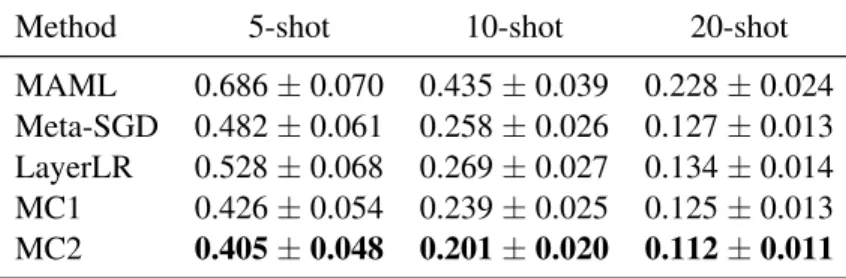
4.4.1 Few-shot regression . . . 44
4.4.2 Few-shot classification on Omniglot . . . 45
4.4.3 Few-shot classification on miniImagenet and tieredImagenet . . . 46
4.4.4 Visualization . . . 47
4.4.5 Few-shot reinforcement learning . . . 48
4.4.5.2 Experimental results . . . 49
CHAPTER 5: LEARNING TO GENERATE GIVEN FEW EXAMPLES . . . 55
5.1 Transformation-Grounded View Synthesis . . . 58
5.1.1 Disocclusion-aware Appearance Flow Network . . . 59
5.1.1.1 Visibility map . . . 60
5.1.1.2 Symmetry-aware visibility map . . . 61
5.1.1.3 Background mask . . . 61
5.1.2 View Completion Network . . . 62
5.1.2.1 Loss networks. . . 63
5.2 Experiments . . . 64
5.2.1 Training Setup . . . 64
5.2.2 Results . . . 65
5.2.2.1 Comparisons . . . 67
5.2.2.2 Evaluation of the Loss Networks . . . 68
5.2.3 360 degree rotations and 3D reconstruction . . . 69
5.2.4 3D Object Rotations in Real Images . . . 70
5.3 Related Work . . . 71
5.3.1 Geometry-based view synthesis . . . 71
5.3.2 Image generation networks . . . 72
CHAPTER 6: APPENDICES . . . 76
6.1 Meta-Trackers . . . 76
6.1.1 More visualizations of response maps in MetaCREST . . . 76
6.1.2 Detailed results on VOT2016 . . . 76
6.1.3 Detailed results on OTB2015 . . . 76
6.2 Meta-Curvature . . . 86
6.2.2 Experimental setup . . . 87
6.2.2.1 Few-shot classification . . . 87
6.2.2.2 Few-shot reinforcement learning . . . 88
6.3 Learning to generate given few examples . . . 89
6.4 Detailed Network Architectures . . . 89
6.5 More examples . . . 89
6.6 Test results on random backgrounds . . . 89
6.7 Arbitrary transformations with linear interpolations of one-hot vectors . . . 89
6.8 More categories . . . 90
LIST OF TABLES
Table 3.1 – Quantitative results on VOT2016 dataset. The numbers in legends repre-sent the number of iterations at the initial frame. EAO (expected average overlap) - 0 to 1 scale, higher is better. A (Accuracy) - 0 to 1 scale, higher is better. R (Robustness) - 0 to N, lower is better. We ran each tracker 15
times and reported averaged scores following VOT2016 convention. . . 27 Table 3.2 – Speed and performance of the initialization: The right table shows the losses
of estimated response map in MetaCREST. The left table shows the ac-curacy of image patches in MetaSDNet. B (Before) - the performance of the initial frame before training, A (After) - the performance of the initial frame after training, LH (Lookahead) - the performance of next 5 frames
after training, Time - wall clock time to train in seconds . . . 29
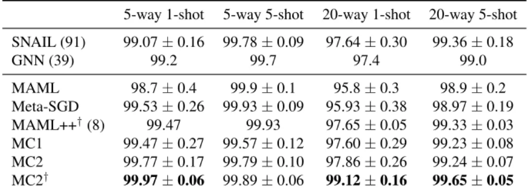
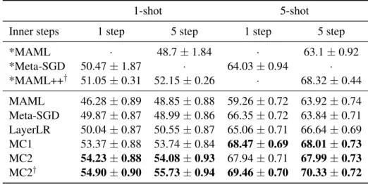
Table 4.1 – Few-shot regression results on sinusoidal functions. . . 44 Table 4.2 – Few-shot classification results on Omniglot dataset.†denotes 3 model
en-semble. . . 45 Table 4.3 – Few-shot classification results on miniImagenet test set (5-way
classifi-cation) with baseline 4 layer CNNs. * is from the original papers.†denotes
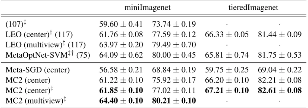
3 model ensembles. . . 47 Table 4.4 – The results on miniImagenet and tieredImagenet with WRN-28-10
fea-tures. ‡indicates that both meta-train and meta-validation are used
dur-ing meta-traindur-ing. . . 48
Table 5.1 – We compare our method (TVSN(DOAFN)) to several baselines: (i) a single-stage encoder-decoder network trained with different loss functions: L1 (L1), feature reconstruction loss using VGG16 (VGG16), adversarial (Adv), and combination of the latter two (VGG16+Adv), (ii) a variant of our
ap-proach that does not use a visibility map (TVSN(AFN)). . . 65
Table 6.1 – Detailed results of MetaCREST on VOT2016 — Accuracy. . . 78 Table 6.2 – Detailed results of MetaCREST on VOT2016 — Robustness (The
num-ber of failures). . . 79 Table 6.3 – Detailed results of MetaSDNet on VOT2016 — Accuracy. . . 80 Table 6.4 – Detailed results of MetaSDNet on VOT2016 — Robustness (The number
Table 6.5 – Detailed results of MetaCREST on OTB2015 (BasketBall — Girl). . . 82
Table 6.6 – Detailed results of MetaCREST on OTB2015 (Girl2 — Woman). . . 83
Table 6.7 – Detailed results of MetaSDNet on OTB2015 (BasketBall — Girl). . . 84
LIST OF FIGURES
Figure 3.1 – Our meta-training approach for visual object tracking: A computational graph for meta-training object trackers. For each iteration, it gets the gra-dient with respect to the loss after the first frame, and a meta-updater up-dates parameters of the tracker using those gradients. For added stabil-ity and robustness a final loss is computed using a future frame to com-pute the gradients w.r.t parameters of meta-initializer and meta-updater.
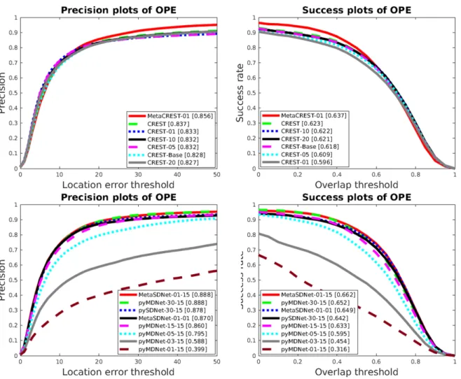
More details in Section 3.1. . . 16 Figure 3.3 – Precision and success plots over 100 sequences in OTB2015 dataset with
one-pass evaluation (OPE). For CREST (top row),The numbers in leg-ends represent the number of iterations at the initial frame, and all used 2 iterations for the subsequent model updates. For MDNet experiments (bottom row), 01-15 means, 1 training iterations at the initial frame and
15 training iterations for the subsequent model updates. . . 28 Figure 3.4 – Visualizations of response maps in CREST: Left three columns represents
the image patch at the initial frame, response map with meta-learned ini-tial correlation filtersθ0f, response map after updating 1 iteration with learnedα, respectively. The rest of seven columns on the right shows
re-sponse maps after updating the model up to 10 iterations. . . 30 Figure 3.5 – Qualitative examples: tracking results at early stage of MotorRolling (top)
and Bolt2 (bottom) sequences in OTB2015 dataset. Color coded boxes:
ground Truth (Red), MetaCREST-01 (Green) and CREST (Blue). . . 31
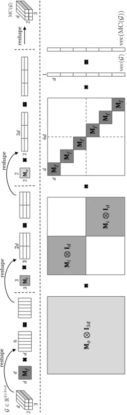
Figure 4.1 – An example of meta-curvature computational illustration withG ∈R2×3×d .
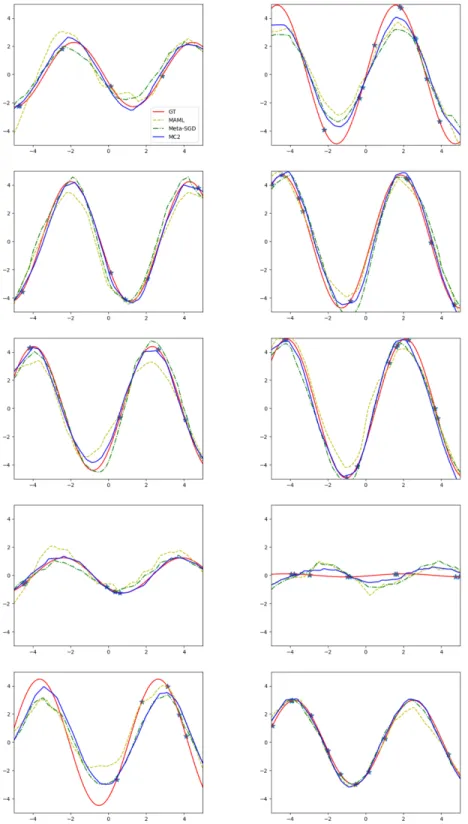
Top: tensor algebra view, Bottom: matrix-vector product view. . . 36 Figure 4.2 – Qualitative results of few-shot regression on sinusoidal functions. The
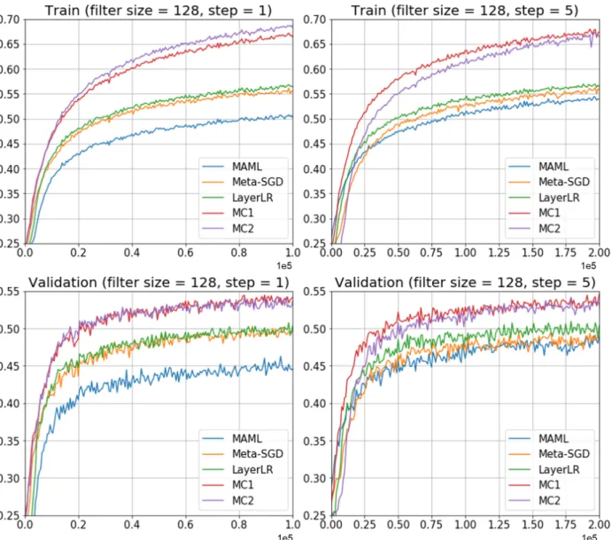
left column - 5 shot, The right column - 10 shot . . . 50 Figure 4.3 – Experimental results of one-shot classification. Top row - training
accu-racy after the model update (1 or 5 steps). Bottom row - validation ac-curacy after the model update (1 or 5 steps). Y-axis: acac-curacy. X-axis:
meta-training iterations. . . 51 Figure 4.4 – Experimental results of one-shot classification. Top row - training
accu-racy after the model update (1 or 5 steps). Bottom row - validation ac-curacy after the model update (1 or 5 steps). Y-axis: acac-curacy. X-axis:
Figure 4.5 – Visualization of meta-curvature matrices. We clipped the values[−1,1]
for better visualization (Best viewed in color) . . . 53 Figure 4.6 – Reinforcement learning experimental results. Y-axis: rewards after the
model updates. X-axis: meta-training steps. We performed at least three
runs with random seeds and the curves are averaged over them. . . 54
Figure 5.1 – Results on test images from 3D ShapeNet dataset (15). 1st-input, 2nd-ground truth. From 3rd to 6th are deep encoder-decoder networks with different losses. (3rd-L1norm (133), 4th-feature reconstruction loss with pretrained VGG16 network (60; 74; 137; 73), 5th-adversarial loss with feature matching (41; 108; 118; 24), 6th-the combined loss). 7th-appearance
flow network (AFN) (157).8th-ours(TVSN). . . 57 Figure 5.2 – Transformation-grounded view synthesis network(TVSN). Given an
in-put image and a target transformation (5.1.1), our disocclusion-aware ap-pearance flow network (DOAFN) transforms the input view by relocat-ing pixels that are visible both in the input and target view. The image completion network, then, performs hallucination and refinement on this intermediate result(5.1.2). For training, the final output is also fed into two different loss networks in order to measure similarity against ground
truth target view (5.1.2.1). . . 59 Figure 5.3 – Visibility maps for different rotations: the first column in the first row
is an input image. Remaining columns show output images and corre-sponding masks for rotations from 20 to 340 degrees in 20 degree inter-vals. The second, third and fourth rows show visibility mapsMvis,
symmetry-aware visibility mapsMs-vis, and background masksMbg, respectively.
The input image is in the pose of 0 elevation and 20 azimuth. The vis-ibility maps for the rotations from 160 to 340 show the largest difference betweenMvisandMs-vis. For example,Ms-visshows the opposite side of
the car as visible and allows it to be filled in by the network based on the
visible side. . . 60 Figure 5.4 – Results on synthetic data from ShapeNet. We show the input, ground truth
output (GT), results for AFN and our method (TVSN) along with theL1 error. We also provide the intermediate output (visibility map and
out-put of DOAFN). . . 66 Figure 5.5 – When a visibility map is not utilized (TVSN(AFN)), severe artifacts
ob-served in the AFN output get integrated into the final results. By mask-ing out such artifacts, our method (TVSN(DOAFN)) relies purely on the
Figure 5.6 – We evaluate the effect of using only parts of our system, VGG16 in TVSN(VGG16), and adversarial loss in TVSN(Adversarial), as opposed to our method,
TVSN(VGG16+Adversarial) that uses both. . . 69
Figure 5.7 – Results of 360 degree rotations . . . 74
Figure 5.8 – We run a multi-view stereo algorithm to generate textured 3D reconstruc-tions from a set of images generated by AFN and our TVSN approach. We provide the reconstructions obtained from ground truth images (GT) for reference. . . 75
Figure 5.9 – We show novel view synthesis results on real internet images along with the predicted visibility map and the background mask. . . 75
Figure 6.1 – More visualizations of response maps in MetaCREST: Left three columns represents a cropped image centered on the target at the initial frame, re-sponse map with meta-learned initial correlation filtersθ0, response map after updating 1 iteration with meta-learnedα, respectively. The rest of six columns on the right shows response maps of CREST after updating the model up to 10 iterations. . . 77
Figure 6.2 – Transformation-grounded view synthesis network architecture . . . 91
Figure 6.3 – Results on test images from the car category (15). 1st-input, 2nd-ground truth. From 3rd to 6th are deep encoder-decoder networks with differ-ent losses. (3rd-L1 norm (133), 4th-feature reconstruction loss with pre-trained VGG16 network (60; 74; 137; 73), 5th-adversarial loss with fea-ture matching (41; 108; 118), 6th-the combined loss). 7th-appearance flow network (AFN) (157).8th-ours(TVSN). . . 92
Figure 6.4 – Results on test images from the car category (15). 1st-input, 2nd-ground truth. From 3rd to 6th are deep encoder-decoder networks with differ-ent losses. (3rd-L1 norm (133), 4th-feature reconstruction loss with pre-trained VGG16 network (60; 74; 137; 73), 5th-adversarial loss with fea-ture matching (41; 108; 118), 6th-the combined loss). 7th-appearance flow network (AFN) (157).8th-ours(TVSN). . . 93
Figure 6.5 – Test results on synthetic backgrounds . . . 94
Figure 6.6 – Test results of linear interpolation of one-hot vectors . . . 95
CHAPTER 1: AUTOMATIC MACHINE LEARNING (META-LEARNING)
Deep learning has played a key role to make remarkable progress on artificial intelligence (AI) over the last decade. It has been successfully used on a variety of tasks in AI, e.g. image recognition (116) and generation (41), speech recognition and generation (140) , machine trans-lation, playing challenging games (92; 126), and so on. There have been many enabling factors behind this incredible success, such as large amount of data (116), powerful computations, some of algorithmic breakthroughs (48; 55), and open sourcing efforts from both academia and indus-tries (3; 104).
Thanks to this collective efforts toward building AI systems, we hear a myriads of successful stories. However, developing and applying current deep learning techniques to many real world problems is still challenging task itself and in most cases it requires the knowledge from human experts on this domain. Furthermore, human experts very often depends on the trial-and-error approach, which is time consuming and tedious repetitive process. Automatic machine learning (or meta-learning) has emerged from this motivation.
re-quires often more than a day or week and there are too many factors that would potentially affect the eventual performance.
The most distinctive feature of meta-learning is that it aims to achieve better generalization in a principled way. Instead of resting on empirical intuition to adjust training configurations through cross-validation, we define a meta-objective function, which maximizes the generaliza-tion performance, to find the best training configurageneraliza-tions. As opposed to optimizageneraliza-tion methods that usually aim to reach to the best training loss value, meta-learning’s main objective is the model’s generalization ability and less focus on training loss.
In this chapter, we introduce recent progress on this domain and provide high-level overview. We also provide in-depth introduction of gradient-based meta-learning, which will be used for later chapters.
1.1 Meta-learning
1.2 Categorization
This is an emerging field in machine learning community and many recent works have slightly different purpose and training setups. In this section, we categorize them into few representative meta-training algorithms and training setups.
1.2.1 Training algorithm
1.2.1.1 Bayesian optimization
trad-ing off exploration and exploitation. It has been very effective, especially for low dimensional hyperparameters, e.g. learning rate and this obtained new state-of-the-art results in tuning hy-perparameters for image classification tasks (58). However, it is still early stage to apply for high-dimensional hyperparameters, e.g. initialization of the network parameters. For in-depth introduction to this, we refer to the tutorial (125).
1.2.1.2 Reinforcement learning
To scale up high-dimensional hyperparameters, the reinforcement learning has been success-fully used to find a network architecture (158; 159). We can optimize a network architecture that maximize validation performance and we can treat validation losses as negative rewards and we typically use policy gradients to optimize the meta-network that generates the network architec-ture. It also has an advantage over gradient-based methods. It does not have to unroll the large number of training steps in gradient descent steps. Thanks to recent advances in deep reinforce-ment learning, it obtained new state-of-the-art results on variety of tasks with the architecture founded and it gave us interesting aspects of designing network architecture.
1.2.1.3 Evolutionary method
1.2.1.4 Gradient-based methods
Thanks to recent advances in automatic differentiation techniques, it has been popular choice to obtain gradient through unrolling gradient descent steps. Although it has potential issues such as short-horizon bias (153) and computational complexity for large unrolling steps (84), it has been successfully used in hyperparameter search (84) and meta-training initialization of the net-works for few-shot classification and reinforcement learning setup (31). Throughout this disserta-tion, we explore and discuss the effectiveness of gradient-based methods focusing on learning the initialization of the parameters and how to adapt the gradients for better generalization and faster convergence.
1.2.2 Training setup
In meta-training, we collect few training episodes, a.k.a mini-batches in usual training setup, and construct the batches to optimize for meta-objective functions. We can differentiate the ex-isting meta-learning works into two different scenarios. First, we can provide different tasks for every training episodes. In this case, we are optimizing training configurations for the tasks from a task distribution. We hope the resulting configurations or hyperparameters will generalize well for a new task, which can be quite different than the tasks in the meta-training.
distribution. The resulting meta-trained model can be effectively used for similar tasks but unseen categories and images.
Second, there has been many works that optimize the training configurations for a particular task. In this setup, we provide same task for every training episodes, which aims to learn an op-timal training configuration that optimize generalization performance for the task. For example, hyperparameter optimization (128; 84) can fall into this category. Every training episodes, they look at the validation loss, it determines which hyperparameters and how to adjust values based on uncertainty in the hyperparameter space through gaussian process (128) or gradients from the validation loss (84).
1.3 Model-agnostic meta-learning (MAML)
MAML aims to find a transferable initialization (a prior representation) of any model such that the model can adapt quickly from the initialization and produce good generalization perfor-mance on new tasks. It is general and model-agnostic, which it can be directly applied to any learning problem and model that is trained with a gradient descent algorithm. The meta-objective is defined as validation performance after one or few step gradient updates from the model’s ini-tial parameters. By using gradient descent algorithms to optimize the meta-objective, its training algorithm usually takes the form of nested gradient updates: inner updates for model adaptation to a task and outer-updates for the model’s initialization parameters. More formally,
min
θ Eτi[L τi
val θ−α∇L
τi
tr(θ)
| {z }
inner udpate
], (1.1)
whereLτi
val(·)denotes a loss function for a validation set of a taskτi, andLτtri(·)for a training set,
orLtr(·)for brevity. The inner update is defined as a standard gradient descent with fixed learning
Starting from randomly initialized model parametersθ0, the model parameters after after one gradient descent step can be written as
θ1 =θ0−α∇θLtr(θ0) (1.2)
In order to optimize meta-objective function that minimize validation loss, we can take the gradient of validation loss w.r.t the initial parametersθ0. Once we have this gradient (also called as meta-gradient), we update the initial model’s parametersθ0with gradient descent algorithms. Therefore, simple update rules for meta-training model’s initial parameters with a single gradient steps in inner update can be written as follows.
θ0 =θ0−β∇θ0Lval(θ1) (1.3)
=θ0−β∇θ0Lval(θ0−α∇θLtr(θ0)) (1.4)
=θ0−β∇θLval(θ1)(I−α∇2θLtr(θ0)) (1.5)
where,βandαare the learning rates for outer loop and inner loop respectively. This meta-gradients requires the meta-gradients of the gradient, which has higher order gradient terms, e.g. sec-ond order gradients in this example. It is not scalable to compute this gradients manually. In addition, computing higher order gradients are often infeasible especially for large deep neural networks that have millions of model parameters. However, we do not have to explicitly compute or maintain the second order gradients here because eventually we will be computing matrix-vector product∇θLval(θ1)∇2θLtr(θ0), and we can use trick from (106) that allows us to easily compute this by using automatic differentiation software packages (3; 104).
Several variations of inner update rules were suggested. Meta-SGD (78) suggested coordinate-wise learning rates,θ−α◦ ∇Ltr, whereαis the learnable parameters and◦is element wise product.
CHAPTER 2: BACKGROUND
In this chapter, we present some of background materials that are useful to formalize and understand the proposed methods in the chapter 4. First, we review the tensor algebra to formal-ize the proposed method. Tensor algebra is a great mathematical tool to translate complicated tensor operations into concise notation. In addition, there are many properties that we can easily use to understand the proposed methods. Secondly, we introduce some second-order optimiza-tion algorithms that are commonly used in training deep neural networks. This will be useful to understand the relationship between the proposed method and existing optimization algorithms.
2.1 Tensor Algebra
We review basics of tensor algebra that will be used to formalize the proposed method. We refer the reader to (67) for a more comprehensive review. Throughout the paper, tensors are defined as multidimensional arrays and denoted by calligraphic letters, e.g.Nth-order tensor,
X ∈ RI1×I2×···×IN. Matrices are second-order tensors and denoted by boldface uppercase, e.g. X∈RI1×I2.
2.1.1 Fibers
Fibers are a higher-order generalization of matrix rows and columns. A matrix column is a mode-1fiber and a matrix row is a mode-2fiber. For a third order tensorX, the mode-1 fibers of
2.1.2 Tensor unfolding
Also known asflattening (reshaping)ormatricization, is the operation of arranging the el-ements of an higher-order tensors into a matrix. The mode-nunfolding of aNth-order tensor
X ∈ RI1×I2×···×IN, arranges the mode-n fibers to be the columns of the matrix, denoted by X[n] ∈ RIn×IM, whereIM = Qk6=nIk. The elements of the tensor,Xi1,i2,...,iN are mapped to X[n]in,j, wherej = 1 +
PN
k6=n,k=1(ik−1)Jk, withJk= Qk−1
m=1,m6=nIm.
2.1.3 n-mode product
It defines the product between tensors and matrices. Then-mode product of a tensorX ∈
RI1×I2×···×IN with a matrixM∈RJ×In is denoted byX ×nMand computed as
(X ×nM)i1,...,in−1,j,in+1,...,iN = In X
in=1
Xi1,i2,...,iNMj,in. (2.1)
More concisely, it can be written as(X ×nM)[n] =MX[n]∈RI1×···×In−1×J×In+1×···×IN. Despite cumbersome notation, it is simplyn-mode unfolding (reshaping) followed by matrix multiplica-tion.
2.1.4 Tucker decomposition
We can decompose a tensorX ∈ RI1×I2×···×IN into a low rank coreG ∈
RR1×R2×···×RN
through projection along each of its modes by projection factors(U(0),· · ·,U(N)), withU(k) ∈
RRk×Ik, k ∈(0,· · · , N). Formally, it can be written as
X =U ×1U(1)×2U(2)· · · ×N U(N). (2.2)
2.2 Gradient descent methods
We also review of basics of gradient descent methods. We refer the reader to (99) for a more comprehensive review. Gradient descent methods, more specifically stochastic variations, have dominated for training large scale deep neural networks. With reverse-mode automatic differenti-ation technique, a.k.a back-propagdifferenti-ation algorithm, we can easily compute the gradients and apply simple mini-batch stochastic gradient descent algorithm. It turns out stochastic variations have a great generalization performance compared to batch gradient descent (98).
2.2.1 First order methods
The most notable example of first order methods for deep learning is the stochastic gradient descent with momentum. First order methods cannot capture the higher-order dependencies between the parameters (by definition), and it focuses on the history of gradients for individual components. With momentum, it computes the gradients based on exponential average over certain amount of history for each elements of gradients. Therefore, some local gradient with specific mini-batch gave a bad direction, it has a chance to fix this based on the history of the gradients. ADAM (66) combines second order information to accelerate the convergence speed. It maintains the history of inverse of square of gradients for every elements, which then will be used to multiply the current gradients. We can interpret this as a diagonal approximation of online natural gradient descent algorithm, which will be discussed in the next section.
2.2.2 Second order methods
atθtinstead of original loss function. We provide two representative algorithms, Newton method and natural gradient method.
2.2.2.1 Newton method
We perform second-order taylor approximation of loss function atθt.
L(θt+d)≈L(θt) +∇L(θt)>d+
1 2d
>∇2
θL(θt)d, (2.3)
wheredis the direction we take to minimize the loss. Then, we minimize this surrogate quadratic function w.r.tdinstead of original loss function. We take the gradient w.r.tdand set it to zero, we obtain analytic solution
− ∇2θL(θt)−1∇θL(θt) = argmin
d
L(θt) +∇L(θt)>d+1 2d
>
. (2.4)
And we can recover well-known newton update rule
θt+1 =θt−α∇2θL(θt)−1∇θL(θt). (2.5)
2.2.2.2 Natural gradient method
Natural gradient method was invented in (6) and it has been widely adopted in training deep neural networks. It finds a steepest descent direction in distribution space rather than parame-ter space by measuring KL-divergence as a distance metric. For example, if we define the loss function as negative log likelihood, e.g. a supervised classification taskL(θ) = E(x,y)∼p(x,y)[
−logp(y|x;θ)], then the empirical Fisher information matrix can be defined asF=E(x,y)∼p(x,y)[
∇θlogp(y|x;θ)∇θlogp(y|x;θ)>]. Let us consider a constrained optimization problem
argmin d
In this optimization problem, we seek to find a directiondsuch that it minimize the loss value after an update with the constraint preventing from you deviating too much from the current iter-ation. It is encoded by setting a maximum KL divergence of a certain constantc. We can form a Lagrangian to convert into unconstrained optimization problem and perform local approximation.
argmin d
L(θt) +∇θL(θt)>d+λ(KL(pθt||pθt+d)−c) (2.7) ≈argmin
d
L(θt) +∇θL(θt)>d+λ(1 2d
>
Fd−c). (2.8)
Equation 2.8 comes from the fact that we perform second order approximation of KL divergence (Note that the Hessian of KL divergence between two different distribution is Fisher information). Similar to the derivation of Newton method, if we take the gradient w.r.t.dand set it to zero, we can obtain the solution of this surrogate function and we reach to natural gradient update rule
θt+1 =θt−αF−1∇L(θt). (2.9)
2.2.2.3 Kronecker-factored approximate curvature
CHAPTER 3: META-TRACKER: FAST AND ROBUST ONLINE ADAPTATION FOR VISUAL OBJECT TRACKERS
In this chapter, we improve the state-of-the-art visual object trackers with meta-learning strategies. Visual object tracking is a task that locates target objects precisely over a sequence of image frames given a target bounding box at the initial frame. In contrast to other object recogni-tion tasks, such as object category classificarecogni-tion and detecrecogni-tion, in visual object tracking, instance-level discrimination is an important factor. For example, a target of interest could be one particu-lar person in a crowd, or a specific product (e.g. coke can) in a broader category (e.g. soda cans). Therefore, an accurate object tracker should be capable of not only recognizing generic objects from background clutter and other categories of objects, but also discriminating a particular target among similar distractors that may be of the same category. Furthermore, the model learned dur-ing trackdur-ing should be flexible to account for appearance variations of the target due to viewpoint change, occlusion, and deformation.
One approach to these challenges is applying online adaptation. The model of the target during tracking, e.g. DCF (discriminative correlation filter) or binary classifier (the object vs backgrounds), is initialized at the first frame of a sequence, and then updated to be adapted to target appearance in subsequent frames (96; 129; 22; 19; 50; 82; 62; 14). With the emergence of powerful generic deep-learning representations, recent top performing trackers now leverage the best of both worlds: deep learned features and online adaptation methods. Offline-only trackers trained with deep methods have also been suggested, with promising results and high speed, but with a decrease in accuracy compared to state-of-the-art online adaptive trackers (13; 49; 132), perhaps due to difficulty finely discriminating specific instances in videos.
pre-trained features have proven to be a powerful and broad representation that can recognize many generic objects, enabling effective training of target models to focus on the specified target in-stance. Although this type of approach has shown the best results so far, there remain several important issues to be resolved.
First, very few training examples are available. We are given a single bounding box for the target in the initial frame. In subsequent frames, trackers collect additional images, but many are redundant since they are essentially the same target and background. Furthermore, recent trends towards building deep models for target appearance (96; 129) make the problem more challenging since deep models are known to be vulnerable to overfitting on small datasets. As a consequence, a target model trained on top of deeply learned features sometimes suffers because it overfits to background clutter, small parts or features of the target, or noise. Many recent stud-ies have proposed various methods to resolve these issues. Some include using a large number of positive and negative samples with aggressive regularizers (96), factorized convolution (19), spatio-residual modules (129), or incorporating contextual information (94).
Second, most state-of-the-art trackers spend a significant amount of time on the initial train-ing stage (96; 129; 19). Although many works have proposed fast traintrain-ing methods (19; 50), this still remains a bottleneck. In many practical applications of object tracking, such as surveillance, real-time processing is required. Depending on the application, falling behind on the initial frame could mean failure on the whole task. On the other hand, an incompletely trained initial target model could affect performance on future frames, or in the worst case, result in failures on all subsequent frames. Therefore, it is highly desirable to obtain the robust target model very quickly at the initial frame.
it does not necessarily mean it would work well for future frames. Instead, we suggest to use error signals from future frames. During the meta-training phase, we aim to find a generic initial representation and gradient directions that enable the target model to focus on features that are useful for future frames. Also, this meta-training phase helps to avoid overfitting to distractors in the current frame. In addition, by enforcing the number of update iterations during meta-training, the resulting networks train significantly faster during the initialization.
Our proposed approach can be applied to any learning based tracker with minor modifications. We select twostate-of-the-art trackers, MDNet (96), from the classifier based tracker (tracking-by-detection) category, and CREST (129), a correlation based tracker. Experimental results show that our meta-learned version of these trackers can adapt very quickly—just one iteration—for the first frame while improving accuracy and robustness. Note that this is done even without em-ploying some of the hand engineered training techniques, sophisticated architectural design, and hyperparameter choices of the original trackers. In short, we present an easy way to make very good trackers even better without too much effort, and demonstrate its success on two different tracking architectures, indicating potentially general applicability.
3.1 Meta-Learning for Visual Object Trackers
In this section, we explain the proposed generalizable meta-training framework for visual object trackers. The details for applying this to each tracker are found in Section 3.2.
3.1.1 Motivation
Figure 3.1: Our meta-training approach for visual object tracking: A computational graph for meta-training object trackers. For each iteration, it gets the gradient with respect to the loss after the first frame, and a meta-updater updates parameters of the tracker using those gradients. For added stability and robustness a final loss is computed using a future frame to compute the gradients w.r.t parameters of meta-initializer and meta-updater. More details in Section 3.1.
images are then stored in the database, and the models are regularly updated with collected data according to their own strategies.
A key motivation is to incorporate these actual tracking scenarios into the meta-learning process. The eventual goal of trackers is to predict the target locations in future frames. Thus, it would be desirable to learn trackers with this eventual goal. For example, if we could look at variations in future frames, then we could build more robust target models and prevent them from overfitting to the current target appearance or background clutter. We can take a step back and observe trackers running on videos, see if the trackers generalize well, and find a reason why they become distracted and adjust the adaptation procedure accordingly.
3.1.2 A general online tracker
Algorithm 1Meta-training object trackers algorithm
Input: Randomly initializedθ0 andα, training datasetD
Output: θ0∗andα∗
1: whilenot convergeddo
2: gradθ0,gradα =~0 .Initialize to zero vector
3: for allk∈ {0, . . . , Nmini−1}do
4: S, j, δ ∼p(D) .Sample a training example
5: θ00 =θ0
6: for allt∈ {0, . . . , T −1}do 7: yˆj =F(xj, θ0t)
8: θ0t+1 =θ0t−α ∇θt
0L(yj,yjˆ;θ
t 0) 9: θ1 =θ0T
10: yˆj+δ=F(xj+δ, θ1) .Apply to a future frame
11: gradθ0 =gradθ0 +∇θ0L(yj+δ,yˆj+δ) .Accumulate the gradients
12: gradα =gradα+∇αL(yj+δ,yj+δˆ )
13: θ0 =Optimizer(θ0,gradθ0) .Updateθ0
14: α =Optimizer(α,gradα) .Updateα
the tracker parametersθand produces an estimateyˆof the label, e.g. a response map or a loca-tion in the frame that indicates the target posiloca-tion. Forinitialization,x0 from the initial frame I0with specifiedy0, we (approximately) solve forθ1(x0, y0), orθ1for brevity, with respect to a loss,L(F (x0, θ1), y0), measuring how well the model predicts the specified label. Forupdates during tracking, we take the parametersθj from framej −1and findyˆj =F(xj, θj), then findθj+1 with respect to a loss. Then, we may incorporate transformingyˆj into a specific estimate of the target location as well as temporal smoothing, etc. We can write the tracking process initialized withx0 andy0 in an initial frame and then proceeding to track and update for framesI1. . . In asTrack (θ1(x0, y0), I1, . . . , In)and its output asyˆn, an estimate of the label in thenth frame (indicating target position) andθn+1, the model parameters after thenth frame.
3.1.3 Meta-training algorithm
itera-tions of a update functionM parameterized byα. Another goal is that the resulting tracker be accurate and robust on later frames.
The gradient-descent style update functionM is parameterized byα:
M(θ,∇θL;α) =θ−α ∇θL , (3.1)
whereαis the same size as the tracker parametersθ(78),Lis a loss function, andis element-wise product. αcould be a scalar value, which might be either learnable (4) or manually fixed (31). We empirically found that having per parameter coefficients was the most effective in our set-tings.
Our meta-training algorithm is to find a goodθ0 andαby repeatedly sampling a video, per-forming initialization, applying the learned initial model to a frame slightly ahead in the se-quence, and then back-propagating to updateθ0 andα. Applying the initial model to a frame slightly ahead in the sequence has two goals, the model should be robust enough to handle more than frame-to-frame variation, and if so, this should make updates during tracking fast as well if not much needs to be fixed.
After sampling a random starting frame from a random video, we perform optimization for initialization starting withθ00 =θ0 given the transformed input and output pair,(xj, yj). A step of optimization proceeds as
θi+10 =M(θ0i,∇θi
0L(yj, F(xj, θ
i
0))). (3.2)
This step can be repeated up to a predefined number of timesT to find,θ1(xj, yj) = θT0. Then, we randomly sample a future frameIj+δ and evaluate the model trained on the initial frame on that future frame to produce:yˆj+δ=F(xj+δ, θ1).
parameters. The objective function is defined as
θ0∗, α∗ = argmin
θ0,α
ES,j,δ[L(yj+δ,yˆj+δ)]. (3.3)
We used the ADAM (66) gradient descent algorithm to optimize. Note thatθ0 andαare fixed across different episodes in a mini-batch, butθ1
0, . . . , θ0T are changed over every episode. To compute gradients of the objective function w.r.tθ0andα, it is required to compute higher-order gradients (the gradients of function of gradients). This type of computation has been exploited in recent studies (31; 84; 89). We can easily compute this thanks to automatic differentiation software libraries (pyt). More details are explained in Algorithm 1.
3.1.4 Update rules for subsequent frames.
Most online trackers, including the two trackers we meta-train (Section 3.2), update the target model regularly to adjust to new examples collected by itself during tracking. We could simply use meta-trainedαto update the model,θj = θj−1 −α ∇θj−1L(only one iteration presented
for brevity). However, it often diverges on longer sequences or the sequences that have very small frame-to-frame variations. We believe this is mainly because we trainαfor fast adaptation at the initial frame, so the values ofαare relatively large, which causes unstable convergence behavior (A similar phenomenon was reported in (4) albeit in a different context). Sinceαis stable when it teams up withθ0, we could define the update rules for subsequent frames asθj =θ0−α ∇θ0L, as
suggested in (4). We could also combine two strategies,θj =β(θj−1−α ∇θj−1L) + (1−β)(θ0−
α ∇θ0L). Although we could resolve unstable convergence behavior with these strategies, none
(a) MetaCREST (b) MDNet vs MetaSDNet
3.2 Meta-Trackers
In this section, we show how our proposed meta-learning technique can be realized in state-of-the-art trackers. We selected two different types of trackers, one from correlation based track-ers, CREST (129), and one from tracking-by-detection based trackers MDNet (96).
3.2.1 Meta-training of correlation based tracker
3.2.1.1 CREST
A typical correlation filter objective is defined as follows.
argmin
f
||y−Φ(x)∗f||2+λ||f||2, (3.4)
argmax
(h,w)
ˆ
y(h, w), (3.5)
whereyˆ = Φ(xnew)∗f, andyˆ(h, w)represents the element ofyˆin(h, w)coordinates. CREST
used a variation of the correlation filter objective, defined as
X
(h,w)∈P
1
|P|(e
y(h,w)|
y(h, w)−yˆ(h, w)|)2+λ||f||2, (3.6)
whereP ={(h, w) | |y(h, w)−yˆ(h, w)| > 0.1}. This would encourage the model to focus on parts that are far from the ground truth values.
By reformulating the correlation filter as a convolutional layer, it can be effectively integrated into an CNN framework (129). This allows us to add new modules easily, since the optimization can be nicely done with standard gradient descent in end-to-end fashion. They inserted spatio-temporal residual modules to avoid target model degradation by large appearance changes. They also devised sophisticated initialization, learning rates, and weight decay regularizers, e.g. 1000 times larger weight decay parameter on spatio-temporal residual modules. Without those bells and whistles, we aim to learn a robust single layer correlation filter via proposed meta-learning process. There are two important issues for plugging CREST tracker into proposed meta-training framework, and we present our solutions in following sections.
3.2.1.2 Meta-learning dimensionality reduction
learn to reduce dimensions of the features. In CREST, we can insert 1x1 convolution layer right after the feature extraction, the weights of this layer are also meta-learnable and jointly trained during the meta-learning process along with the correlation filter. θ0 in proposed meta-training framework, therefore, consists ofθ0d andθ0f, the parameters of dimensionality reduction and the correlation filter, respectively.
3.2.1.3 Canonical size initialization
The size of the correlation filter varies depending on the target shape and size. In order to meta-train a fixed size initialization of the correlation filterθ0f, we should resize all objects to the same size and same aspect ratio. However, it introduces distortion of the target and has been known to degrade recognition performance (79; 112). In order to fully make use of the power of the correlation filter, we propose to use canonical size initialization and its size and aspect ratio are calculated as a mean of the objects in the training dataset. Based on canonical size initial-ization, we warp it to the specific size taylored to the target object for each tracking episodes,
˜
θ0f =Warp(θ0f). We used differentiable bilinear sampling method (57) to pass through gradients all the way down toθ0f.
Putting it all together,F(xj, θ)in our proposed meta-training framework for CREST, now takes an input a cropped imagexj from an input frameIj, pass it through a CNN feature extractor followed by dimensionality reduction (1x1 convolution with the weightθ0d). Then, it warps the correlation filterθ0f, and finally apply warped correlation filterθ˜0f to produce a response mapyˆj (Figure 3.2a).
3.2.2 Meta-training of tracking-by-detection tracker
3.2.2.1 MDNet
the classifier. At the initial frame, it randomly initializes the last fully connected layer, and trains around 30 iterations with a large number of positive and negative patches (Figure 3.2b). Target locations in the subsequent frames are determined by average of bounding box regression outputs of top scoring positive patches. It collects positive and negative samples during the tracking pro-cess, and regularly updates the classifier. Multi-domain pre-training was a key factor to achieve robustness, and they used an aggressive dropout regularizer and different learning rates at differ-ent layers to further avoid overfitting to currdiffer-ent target appearance. Without those techniques (the multi-domain training and regularizers), we aim to obtain robust and quickly adaptive classifier solely resting on the proposed meta-learning process.
3.2.2.2 Meta-training
It can be also easily plugged into the proposed meta-leraning framework. F(xj;θ)takes as input image patchesxj ∈ RN×D from an input frameIj (andyj ∈ {0,1}N is the corre-sponding labels), whereDis the size of the patches andN is the number of patches. Then, the patches go through a CNN classifier, and the loss functionLis a simple cross entropy loss
−PNk=1yjklog(Fk(xj;θ)).
3.2.2.3 Label shuffling
3.3 Related Work
3.3.1 Online trackers
Many online trackers use correlation filters as the back-bone of the algorithms due to compu-tational efficiency and discriminative power. From the early success of the MOSSE tracker (14), a large number of variations have been suggested. (50) makes it more efficient by taking ad-vantage of circulant matrices, further improved by resolving artificial boundary issues (21; 36). Many hard cases have been tackled by using context information (94; 156), short and long-term memory (83; 54), and scale-estimation (20), just to name a few. Recently, deep learning features have begun to play an important role in correlation filters (96; 129; 22; 19; 82; 139; 76). On the other hand, tracking-by-detection approaches typically learn a classifier to pick up the positive image patches wrapping around the target object. Pioneered by (62), many learning techniques have been suggested, e.g. multiple instance learning (9), structured output SVMs (46), online boosting (43), and model ensembles (10). More recently, MDNet (96), with deep features and a deep classifier, achieved significantly higher accuracy.
3.3.2 Offline trackers
Several recent studies have shown that we can build accurate trackers without online adapta-tion (13; 49; 132) due to powerful deep learning features. Siamese-style networks take a small target image patch and a large search image patch, and directly regress the target location (49) or generate a response map (13) via a correlation layer (33). In order to consider temporal informa-tion, recurrent networks have also been explored in (61; 37; 42; 152).
3.3.3 Meta-learning
with meta-learned deep networks. (109) took this idea into few shot or one shot learning prob-lem. It aimed to learn optimal update strategies based on how accurate a learner can classify test images with few training examples when the learner follows the strategies from the meta-learner. Instead of removing existing optimization algorithms, (31) focuses on learning initialization that are most suitable for existing algorithms. (78) further learns parameters of existing optimization algorithms along with the initialization. Unlike approaches introduced above, there also have been several studies to directly predict the model parameters without going through the optimiza-tion process (152; 12; 145).
3.4 Experiments
3.4.1 Experimental setup
3.4.1.1 VOT2016
It contains 60 videos (same videos from VOT 2015 (69)). Trackers are automatically reini-tialized once it drifts off the target: zero overlap between predicted bounding box and the ground truth. In this reset-based experiments, three primary measures have been used, (i)accuracy, (ii) robustnessand (iii)expected average overlap (EAO). The accuracy is defined as average overlap during successful tracking periods. The robustness is defined as how many times the trackers fail during tracking. The expected average overlap is an estimator of the average overlap a tracker is expected to attain on a large collection of short-term sequences.
3.4.1.2 OTB2015
3.4.1.3 Dataset for meta-training
We used a large scale video detection dataset (116) for meta-training both trackers. It con-sists of 30 object categories, which is a subset of 200 categories in the object detection dataset. Since characteristics of the dataset are slightly different from the object tracking dataset, we sub-sampled the dataset. First, we picked a video frame that contains a target object whose size is not larger than 60% of the image size. Then, a training video sequence is constructed by sam-pling all subsequent frames from that frame until the size of the target object reaches 60%. We ended up having 718 video sequences. In addition, for the experiments on OTB2015 dataset, we also used an additional 58 sequences from object tracking datasets in VOT2013,VOT2014,and VOT2015 (70), excluding the videos included in OTB2015, following MDNet’s approach (96). These sequences were selected in the mini-batch selection stage with the probability 0.3. Sim-ilarly, we used 80 sequences from OTB2015, excluding the videos in VOT2016 for the experi-ments on VOT2016 dataset.
3.4.1.4 Baseline implementations
We selected two trackers, MDNet (96) and CREST (129). For CREST, we re-implemented our own version in python based on publicly released code written in MATLAB. We meta-trained our version. For MDNet, the authors of MDNet provide two different source codes, written in MATLAB and python, respectively. We used the latter one and called it as pyMDNet or pySD-Net, depending on pre-training methods. We meta-trained pySDpySD-Net, and call it as MetaSDNet. Note that overall accuracy of pyMDNet is lower than MDNet on OTB2015 (.652 vs .678 in suc-cess rates with overlap metric). For fair comparison, we compared our MetaSDNet to pyMDNet.
3.4.1.5 Meta-training details
Table 3.1: Quantitative results on VOT2016 dataset. The numbers in legends represent the num-ber of iterations at the initial frame. EAO (expected average overlap) - 0 to 1 scale, higher is better. A (Accuracy) - 0 to 1 scale, higher is better. R (Robustness) - 0 to N, lower is better. We ran each tracker 15 times and reported averaged scores following VOT2016 convention.
EAO Acc R
MetaCREST-01 0.317 0.519 0.932
CREST 0.283 0.514 1.083
CREST-Base 0.249 0.502 1.383
CREST-10 0.252 0.509 1.380
CREST-05 0.262 0.510 1.298
CREST-03 0.262 0.514 1.283
CREST-01 0.259 0.505 1.277
(a) The results of MetaCREST
EAO Acc R
MetaSDNet-01 0.314 0.526 0.934
pyMDNet-30 0.304 0.540 0.943 pyMDNet-15 0.299 0.541 0.977 pyMDNet-10 0.291 0.535 0.989 pyMDNet-05 0.254 0.523 1.198 pyMDNet-03 0.184 0.488 1.703 pyMDNet-01 0.119 0.431 2.733
(b) The results of MetaSDNet
the optimizer with learning rate 1e-4. We only updated the last three fc layers for the first 5,000 iterations and trained all layers for the rest of iterations. The learning rate was reduced to 1e-5 after 10,000 iterations, and we trained up to 15,000 iterations. Forα, we initialized to 1e-4, and also used Adam with learning rate 1e-5, then was decayed to 1e-6 after 10,000 iterations. We used mini-batch sizeNmini = 8. For the meta-update iterationT, largerT gave us only small
improvement, so we set to 1. For each training episode, we sample one random future frame uniformly from 1 to 10 ahead. In MetaCREST, we randomly initializedθ0and also used Adam with learning rate 1e-6. Forα, we initialized to 1e-6, and learning rate of Adam was also set to 1e-6.Nmini = 8and meta-training iterations was 10,000 (at 50,000 iterations, the learning rate
was reduced to 1e-7). We used same hyper-parameters for both OTB2015 and VOT2016 exper-iments. For other hyper-parameters, we mostly followed the ones in the original trackers. For more details, the code and raw results will be released.
3.4.2 Experimental results
3.4.2.1 Quantitative evaluation
Figure 3.3: Precision and success plots over 100 sequences in OTB2015 dataset with one-pass evaluation (OPE). For CREST (top row),The numbers in legends represent the number of itera-tions at the initial frame, and all used 2 iteraitera-tions for the subsequent model updates. For MDNet experiments (bottom row), 01-15 means, 1 training iterations at the initial frame and 15 training iterations for the subsequent model updates.
Table 3.2: Speed and performance of the initialization: The right table shows the losses of es-timated response map in MetaCREST. The left table shows the accuracy of image patches in MetaSDNet. B (Before) - the performance of the initial frame before training, A (After) - the performance of the initial frame after training, LH (Lookahead) - the performance of next 5 frames after training, Time - wall clock time to train in seconds
B A LH Time(s)
MetaCREST-01 0.48 0.04 0.05 0.090
CREST-01 0.95 0.82 0.87 0.395
CREST-03 0.95 0.62 0.75 0.424
CREST-05 0.95 0.45 0.63 0.550
CREST-10 0.95 0.24 0.40 0.668
CREST-20 0.95 0.18 0.31 1.048
CREST-65 0.95 0.01 0.30 1.529
B A LH Time(s)
MetaSDNet-01 0.50 0.98 0.97 0.124
pyMDNet-01 0.51 0.56 0.56 0.123 pyMDNet-03 0.51 0.79 0.78 0.373 pyMDNet-05 0.51 0.84 0.84 0.656 pyMDNet-10 0.51 0.95 0.93 1.171 pyMDNet-15 0.51 0.97 0.97 1.819 pyMDNet-30 0.51 0.99 0.98 3.508
upon their counterparts in both precision and success plots with only one iteration for initializa-tion. Detailed results of individual sequences in both of VOT2016 and OTB2015 are presented in Appendix.
We require only one iteration at the initial frame to outperform the original trackers. We also performed the experiments with more than one iteration, but the performance gain was not signif-icant. On the other hand, MDNet takes 30 iterations to converge at the initial frame as reported in their paper, and fewer iterations caused serious performance degradation. This confirms that getting a robust target model at the initial frame is very important for subsequent frames. For CREST, performance drop was not significant as MDNet, but it was still more than 10 iterations to reach to its maximum performance. MDNet updates the model 15 iterations for subsequent frames at every 10 frames regularly (or when it failed, meaning its score is below a predefined threshold).
3.4.2.2 Speed and performance of the initialization
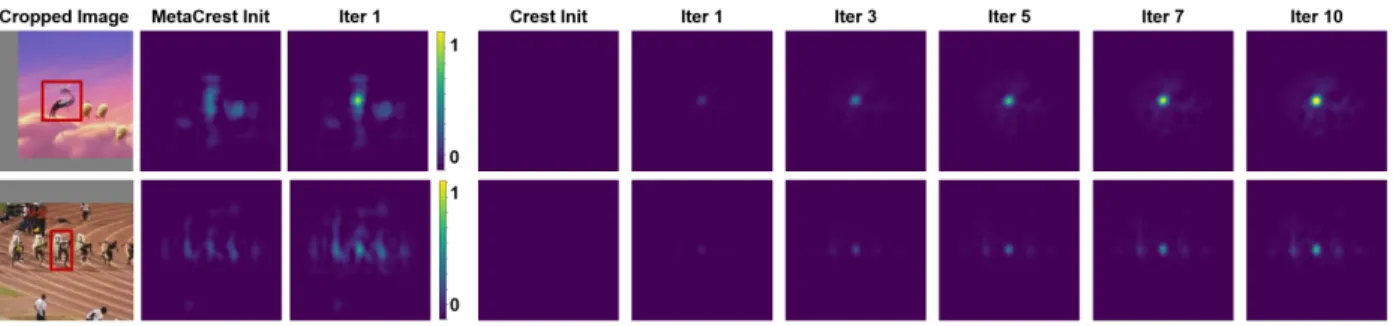
Figure 3.4: Visualizations of response maps in CREST: Left three columns represents the image patch at the initial frame, response map with meta-learned initial correlation filtersθ0f, response map after updating 1 iteration with learnedα, respectively. The rest of seven columns on the right shows response maps after updating the model up to 10 iterations.
comes from PCA at the initial frame. It also depends on the size of the objects. Larger objects lead to larger center cropped images, features, and more computation in PCA.
MDNet requires many positive and negative patches, and also many model update iterations to converge. A large part of the computation comes from extracting CNN features for every patch. MetaSDNet needs only a few training patches and can achieve 30x speedup (0.124 vs 3.508), while improving accuracy. If we used more compact CNNs for feature extractions, the speed could have been in the range of real-time processing. For subsequent frames in MDNet, model update time is of less concern because MDNet only updates the last 3 fully connected lay-ers, which are relatively faster than feature extractors. The features are extracted at every frame, stored in a database, and update the model every 10 frames. Therefore, the actual computation is well distributed across every frames.
per-Figure 3.5: Qualitative examples: tracking results at early stage of MotorRolling (top) and Bolt2 (bottom) sequences in OTB2015 dataset. Color coded boxes: ground Truth (Red), MetaCREST-01 (Green) and CREST (Blue).
formance to CREST-05 after training (0.48 vs 0.45). In original CREST tracker, they train the model until it reaches a loss of 0.02, which corresponds to an average 65 iterations. However, its generalizability at future frames is limited compared to ours (.05 vs .30). Although this is not directly proportional to eventual tracking performance, we believe this is clear evidence that our meta-training algorithm based on future frames is indeed effective, as also supported by overall tracking performance.
3.4.2.3 Visualization of response maps
max-imum is clearly located at the center of the response map. In contrast to MetaCREST, CREST consumes more iterations to produce high response values on the target.
3.4.2.4 Qualitative examples of robust initialization
CHAPTER 4: META-CURVATURE
Despite huge progress in artificial intelligence, the ability to quickly learn from few examples is still far short of that of a human. We are capable of utilizing prior knowledge from past expe-riences to efficiently learn new concepts or skills. With the goal of building machines with this capability,learning-to-learnormeta-learninghas begun to emerge with promising results.
One notable example is model-agnostic meta-learning (MAML) (31; 98), which has shown its effectiveness on various few-shot learning tasks. It formalizeslearning-to-learnas a meta objective function and optimizes it with respect to a model’s initial parameters. Through the meta-training procedure, the resulting model’s initial parameters become a very good prior rep-resentation and the model can quickly adapt to new tasks or skills through one or more gradient steps with a few data examples. Although this end-to-end approach, using standard gradient de-scent as the inner optimization algorithm, was theoretically shown to approximate any learning algorithm (32), recent experiments indicate that the choice of the inner-loop optimization algo-rithm affects performance (78; 8; 44).
few-shot learning setup, because it can overfit easily and quickly. In addition, it may be computa-tionally more expensive since third order derivatives are needed for the outer loop optimizations when the second order derivatives are presented in the inner loop.
In this work, we propose to learn a curvature for better generalization and faster model adap-tation in the meta-learning framework, we callmeta-curvature. The key intuition behind MAML is that there are some representations are broadly applicable to all tasks. In the same spirit, we hy-pothesize that there are some curvatures that are broadly applicable to many tasks. Curvatures are determined by the model’s parameters, network architectures, loss functions, and training data. Assuming new tasks are distributed from the similar distribution as meta-training distribution, there may exist common curvatures that can be obtained through meta-training procedure. The resulting meta-curvatures that are represented by a second-order tensor (matrix), coupled with the simultaneously meta-trained model’s initial parameters, will transform the gradients by mul-tiplying the curvature matrix, such that the updated model has better performance on new tasks with fewer gradient steps. In order to efficiently capture the dependencies between all gradient coordinates for large networks, we design a multilinear mapping consisting of a series of tensor-products to transform the gradients. It also considers layer specific structures, e.g. convolutional layers, to effectively reflects our inductive bias. In addition, meta-curvature can be easily plugged into existing meta-learning frameworks like MAML without additional, burdensome higher-order gradients.
4.1 Method
First, we present a simple and efficient form of the meta-curvature computation through the lens of tensor algebra. Then, we present a matrix-vector product view to provide intuitive idea of the connection to the second order matrices. And, we discuss the relationships to other methods in computational aspects.
4.1.1 Tensor product view
We consider neural networks as our models. With a slight abuse of notation, let the model’s parametersWl ∈
RC
l
out×Cinl ×dland its gradients of loss functionGl ∈ RCoutl ×Cinl ×dl, at each layersl. To avoid cluttered notation, we will omit the superscriptl. We choose superscripts and dimensions with convolutional layers in mind, but the method can be easily extended to other layers, e.g. recurrent layers. Cout, Cin, anddare the number of output channels, the number of input channels, and the filter size respectively.dis height×width in convolutional layers and 1 in fully connected layers. We also define meta-curvature matrices,Mo ∈ RCout×Cout, Mi ∈RCin×Cin, andMf ∈Rd×d. Now a meta-curvature function takes a multidimensional tensor
as an input and has all meta-curvature matrices as learnable parameters.
MC(G) = G ×3Mf ×2Mi×1Mo. (4.1)
fibers in a convolutional filter). Finally, the1-mode product is performed in order to model the dependencies between the gradients of all convolutional filters. Similarly, the gradients of all convolutional filters are updated by linear combinations of gradients of other convolutional filters.
A useful property ofn-mode products is the fact that the order of the multiplications is irrel-evant for distinct modes in a series of multiplications. For example,G ×3 Mf ×2 Mi×1 Mo =
G ×1 Mo×2 Mi ×3Mf. Thus, the proposed method indeed examines the dependencies of the elements in the gradient all together.
4.1.2 Matrix-vector product view
We can also view the proposed meta-curvature computation as a matrix-vector product anal-ogous to that from other second order methods. We can expand the meta-curvature matrices as follows.
d
Mo =Mo⊗ICin⊗Id, (4.2)
c
Mi =ICout ⊗Mi⊗Id, (4.3)
d
Mf =ICout ⊗ICin⊗Mf, (4.4)
where⊗is the Kronecker product,Ik iskdimensional identity matrix, and the three expanded matrices are all same sizedMo,Mci,Mdf ∈ RCoutCind×CoutCind. Now we can transform the gradi-ents with the meta-curvature as
vec(MC(G)) =Mmcvec(G), (4.5)
Figure 4.1 (bottom) shows a computational illustration. Mdfvec(G), which is equivalent com-putation toG ×3Mf, can be interpreted as a giant matrix-vector multiplication with block diagonal matrix, where each block shares same meta-curvature matrixMf. It resembles the block diagonal approximation strategies in some second-order methods for training deep networks, but as we are interested in learning meta-curvature matrices, no approximation is involved. And matrix-vector product withdMoandMciare used to capture inter-parameter dependencies and are equivalent to
2-mode and3-mode products of Eq. 4.1.
4.1.3 Relationship to other methods
We note that the suggested method is computationally related to Tucker decomposition (67), which decomposes a tensor into low rank cores with projection factors and aims to closely recon-struct the original tensor. We maintain full rank gradient tensors, however, and our main goal is to transform the gradients for better generalization. Recently, (68) proposed to learn the projection factors in Tucker decomposition for fully connected layers in deep networks. Again, their goal was to find the low rank approximations of fully connected layers for saving computational and spatial cost.
We also note that the computation of meta-curvature is closely related to Kronecker-factored Approximate Curvature (K-FAC) (85; 45), which approximates the Fisher information matrix by the Kronecker product, e.g. F ≈ A ⊗ G, whereAis computed from the activation of input units andGis computed from the gradient of output units. Its main goal is to approxi-mate the Fisher such that matrix vector products between its inversion and the gradient can be computed efficiently. However, especially in convolutional layers, we found that maintaining A ∈ RCind×Cindwas quite expensive both computationally and spatially even for smaller net-works. In addition, when we applied this factorization scheme to meta-curvature, it tends to easily overfit to meta-training set. On the contrary, we maintain two separated matrices,Mi ∈RCin×Cin
andMf ∈Rd×d, which allows us to avoid overfitting and heavy computation. More importantly,