Sharif University of Technology
Scientia IranicaTransactions A: Civil Engineering http://scientiairanica.sharif.edu
An electromagnetism-like algorithm for solving a
three-dimensional highway alignment problem
A. Mohammadi
aand H. Poorzahedy
b;a. Department of Civil Engineering, Sharif University of Technology, Tehran, Iran.
b. Institute for Transportation Studies and Research, Department of Civil Engineering, Sharif University of Technology, Tehran, Iran.
Received 2 August 2016; received in revised form 4 February 2017; accepted 5 February 2018
KEYWORDS Routing;
Three-dimensional alignment; Meta-heuristic algorithm;
Electromagnetism-like algorithm;
Earthwork-bridge-tunnel costs; User and operator costs;
Reference examples.
Abstract. Road alignment design is an important determinant of the development cost of road networks. On the one side, it aects road construction and maintenance costs, constituting a signicant part of country-wide infrastructure development, management, and operation budget each year. On the other side, it aects road user-related costs of travel time and vehicle use, comprising a signicant portion of the total transportation cost. This study adapts the existing electromagnetism-like meta-heuristic algorithm to solve a three-dimensional highway alignment problem, which explores and nds a good route between two given points on a terrain. It detects the potentials of the given initial routes, which are enhanced and shaped to nd better positions by means of local and global searches. The nal good solution is, then, ne-tuned for a better alignment. Several example problems are designed to show the behavior of the algorithm. The results show that the algorithm satisfactorily maneuvers to by-pass obstacles and build highway structures where necessary. The set of the example problems in this paper may also serve to establish a basis for evaluating the performance of alternative algorithms.
© 2018 Sharif University of Technology. All rights reserved.
1. Introduction
Roads have crucial eects on development; hence, road construction is an important endeavor in all, partic-ularly in the developing, countries. One important aspect of road construction is the specication of its alignment within a real environment. The alignment is then given to the highway designers to ne-tune the horizontal and vertical curves, bridges, tunnels, and other xtures. When we connect two points in a three-dimensional space together by a highway, the benet of this investment is basically accrued and known, and it *. Corresponding author.
E-mail addresses: Mohammadi [email protected] (A. Mohammadi); [email protected]. (H. Poorzahedy) doi: 10.24200/sci.2018.20175
remains to make this connection to minimize the total cost (of construction, maintenance, and operation).
The costs related to a highway may constitute road users' costs (travel time, vehicle operating cost, and accident cost), operator's costs (road construction, maintenance, and operation), and environmental costs (natural land development and adverse environmental eects including the non-users' costs). It may be expected that these costs aect the demand for road use and, thus, the road benet.
There are many constraints in the roadway align-ment and construction, which may be classied as follows:
(a) Technical constraints (maximum slopes, curve radii, safe distances, etc.);
(b) Resource constraints (budget, equipment, and ma-terials);
(c) Environmental constraints (ecological, green-land, wet-land, sensitive areas, etc.);
(d) Archaeological constraints;
(e) Technological constraints (in building bridges, tunnels, etc.);
(f) Standards on adverse eects of road use impacts (noise pollution, visual intrusions, ground vibra-tion, etc.) on human beings and activities; (g) Adverse eects on neighborhood and land-use
integrity.
This paper deals with the following problem. Herein, there is a terrain with known topography and geographical as well as man-made features (lakes, wet-lands, forests, historical buildings, archaeological remains, monuments, preserved areas, etc.). There are two points in the region that are intended to be connected by a new road. The problem is to nd the alignment of this road in the study region, such that it is feasible with respect to the constraints and the objective(s) of road construction is optimized. The alignment may only use the allowable areas of the terrain. In practice, the solution to this problem may not be found by classical optimization methods [1]. The current study has chosen to adapt a new meta-heuristic algorithm, the electromagnetic-like algorithm, to solve this problem.
The purpose of this paper is to adapt an electromagnetism-like algorithm as an eective alter-native approach to solve the three-dimensional road alignment problem. The following are excerpts of the contributions of this paper:
Dening a simple 3D road alignment problem at the strategic level;
Adapting a new electromagnetism-type algorithm to solve the problem;
Dening a exible breaking point concept to pro-duce smoother alignments;
Designing a highway alignment algorithm that works over continuous 3D surfaces;
Designing a procedure that possesses the ability to maneuver in backward directions to nd the optimal alignment;
Designing test problems to evaluate the maneu-vering capabilities of such algorithms, which may form a platform for comparing future algorithmic developments.
This paper rst reviews the literature in Section 2. An overview of the solution procedure is discussed in Section 3, followed by the detailed algorithm in Section 4. The algorithm is calibrated in Section 5 and, then, applied to seven example problems in Section 6.
Section 7 concludes the paper and proposes future research directions.
2. A review of the literature 2.1. General statements
The road alignment or highway routing problem, usu-ally formulated as an optimization problem, started with a two-dimensional (2D, horizontal or vertical) alignment problem. Eventually, it evolved into a three-dimensional (3D) alignment, or routing, problem. It includes both 2D versions of the problem and aspects of the road interaction with its users.
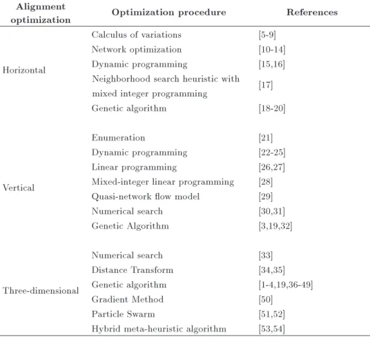
A 2D horizontal alignment problem is involved more than a 2D vertical alignment problem is. This is because the former problem involves political, eco-nomic, social and environmental issues more than the latter, and the latter basically involves techni-cal problems. Thus, in general, optimization proce-dures are more eective in nding a better horizontal alignment than a vertical (alignment) one might be. Nevertheless, there are many algorithms for vertical alignment design, most of which deal with particular road construction cost, such as cuts and lls. Moreover, in vertical alignment design, there is no fear of self-intersecting routes. Kim et al. [1] and Kang et al. [2] presented some previous works in these two areas, which are complemented and summarized in Table 1. In this table, these works are categorized based on the type of the solution procedure employed to solve the problem.
The real-world road alignment problem is, how-ever, three-dimensional. This means that the designer of the alignment has to address:
(a) The planar aspects of the road (that is, the geographical positioning of the road with respect to privately-owned land as well as reserved and preserved historical and environmental sites) and the land acquisition costs;
(b) The prole-related matters of the road (that is, construction aspects of the road such as grades, cut/ll, bridges, and tunnels) and of course the respective construction costs.
Moreover, since a 3D road map is to be imple-mented in the real world, it has to consider:
(c) The aspects of the problem when it undergoes the actual load of trac (that is, the road maintenance costs as well as the user travel costs).
The general formulations of 3D and 2D alignment problems are very much similar to each other, except for the solution procedures employed to solve them. The 3D alignment road problem is usually formulated as an optimization one in which its objective comprises
Table 1. Previous endeavors on highway alignment design. Alignment
optimization Optimization procedure References
Horizontal
Calculus of variations [5-9] Network optimization [10-14] Dynamic programming [15,16] Neighborhood search heuristic with
mixed integer programming [17]
Genetic algorithm [18-20]
Vertical
Enumeration [21]
Dynamic programming [22-25]
Linear programming [26,27]
Mixed-integer linear programming [28] Quasi-network ow model [29]
Numerical search [30,31]
Genetic Algorithm [3,19,32]
Three-dimensional
Numerical search [33]
Distance Transform [34,35]
Genetic algorithm [1-4,19,36-49]
Gradient Method [50]
Particle Swarm [51,52]
Hybrid meta-heuristic algorithm [53,54]
: This is a more up-to-date form of similar tables presented by Kim et al. [1] and Kang et al. [2].
a set of costs related to the users and operator of the road, as well as the environment. Table 1 also summarizes previous works in the 3D road alignment section.
The race in 3D road alignment algorithms appears to be concerned, basically, with computational speed on the one hand, and the denition of a comprehensive objective function and constraint set, on the other hand. The objective functions related to the users and operator of the road may usually be expressed in monetary terms, and the objectives related to the environment may be expressed by rather complex constraints in the problem. Hence, this optimization problem may be better approached by heuristic than conventional routines, as was correctly mentioned by Kim et al. [1]. One good work in the area of 3D road alignment problem belongs to Jong and Schonfeld [3]. Similar to most other researchers, they employed a genetic algorithm to tackle the problem (see also [4]). 2.2. The problem's objective
The cost of roadway alignment includes the following: (a) Location-related costs (CN);
(b) Length-related costs (CL);
(c) Earthwork-related costs (CE);
(d) Bridge and tunnel construction costs (CBrg and
CT nl);
(e) Road maintenance costs (CM);
(f) User-related costs (CU).
The total cost for the alignment (CT) may be
consid-ered the sum of these costs:
CT=CN+CL+CE+CT nl+CBrg+CM+CU: (1)
Note that dierent cost components tend to inu-ence the road alignment dierently. While the costs of cut and ll encourage indirect road alignment options, the costs of pavement, users' travel times, and vehicle fuel tend to encourage shorter and more direct routes. Some cost components are yearly, some depend on a user's demand rate (per year), and some are once in the road life-time which may be converted to yearly costs by suitable conversion factors, using an appropriate minimum attractive rate of return (e.g. [55]).
Despite the fact that many components of the objectives of highway alignment design may be mea-sured by monetary units, some of the works in this area view the problem as multi-objective. Yang et
al. [49] presented one such procedure in which they separated sensitive area impacts from the costs of the agency building the road.
2.3. The problem's constraints
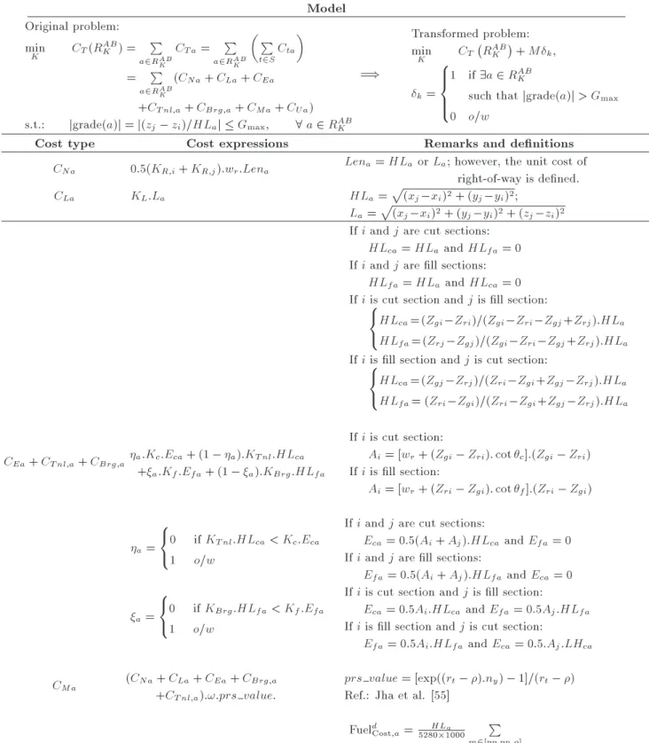
There are considerable constraints on road alignments, which include the minimum radii of horizontal curves, maximum grades, minimum sight distance, and maxi-mum positive grade length. Some constraints may de-ne the allowable made-neuvering area for the alignment. Table 2 presents the model of this study in terms of its objective function and constraints. This table, also, shows details of the computational expressions employed to solve the problem. Table 3 denes the notations used in this model. The road alignment problem in this study is a constrained, shortest path problem in a 3D environment, with the following peculiarities:
(a) In the road alignment problem, the nodes and links are free in (x; y; z)-space, while they are xed and given in the shortest path problem;
(b) The link (or node) costs are given in the latter problem, while we need to decide link types and compute link costs in the former problem;
(c) Road alignment problem has constraints in traversing links, while there is no constraint (like maximum grade) in an ordinary, shortest path problem.
It is worth nothing here that some researchers have also considered geometrical design constraints (such as vertical/horizontal curve design) into the road alignment problems (e.g. [55]). The authors of this paper believe that such minor considerations are not warranted to be included in the road alignment search and should be considered as a next-step activity for the nal/chosen alignment. There are several reasons for this assertion:
(a) Road alignment search is a strategic decision compared to the detailed geometric design features of the problem. As an analogy in the jargon of the network design problem, it is as if major highway decisions are mixed (to build/not to build them) with operational projects (one-way/two-way decisions of streets). The objectives, con-straints, decision exibility, sources of funds, etc. of strategic and tactical decisions are substantially dierent and do not mix well/at all. This is why the subject is referred to as highway alignment or routing (that is, nding the general direction), and not highway design (that involves details such as tangent-spiral-circular combination design, super-elevation, horizontal and vertical sight distances, etc.);
(b) Inclusion of such operational/tactical details would unnecessarily add to the computational complexities of the problem; particularly, the available information and data at strategic levels do not support such actions as highlighted next; (c) The precision of the information and data at
strategic and detailed designs is dierent. At a road alignment level that deals with roads of sev-eral hundred kilometers, we require information accuracy, say, at the 30 m level in planar (x; y) coordinates and the 1 m level in (contour line) elevation, z, while such degrees of precision should be, say, in 1.0 m and 0.1 m, respectively, for detailed designs such as horizontal/vertical curve or maximum grade length;
(d) Finally, there is no point in designing a vast pop-ulation of such routes within meta-heuristic pro-cedures in detail and, then, throwing them away. After all, compared to more rigorous and compu-tationally involved gradient-based methods, one of the merits of meta-heuristic procedures, as an example, is that the former procedures abandon higher computation for nding a \good" solution per iteration with the higher number of solutions, which are found and evaluated swiftly in an iteration.
2.4. The solution procedures
The procedures employed in the literature for the solu-tion of the road alignment problem include numerical methods and meta-heuristic algorithms. The latter form the majority of the procedures employed in the solution of the problem, basically in the form of genetic algorithm, as Table 1 shows. It may be noted in the development of these procedures that researchers are still in search of methods to fulll the following objectives:
(a) Dening it in an appropriate manner, e.g., a single level single objective problem (the most prevalent form of the problem formulation), a single level multi-objective problem (as mentioned below), or a bi-level programming problem [46];
(b) Solving it eectively (higher alignment quality in lower computation time);
(c) Equiping the solution procedure (path nder) with necessary tools and apparatuses to help designers and construction companies to be responsive to the ever-mounting demand on the design and environmental sides of the problem, particularly in this era of high resource and environmental consciousness.
Examples of the above-mentioned tools for solu-tion procedure enhancement include the following:
Table 2. Denition of the 3D highway alignment model and its components in this study. Model
Original problem: min
K CT(R
AB
K ) = P
a2RAB K
CT a= P a2RAB
K
P
t2SCta
= P
a2RAB K
(CNa+ CLa+ CEa +CT nl;a+ CBrg;a+ CMa+ CUa) s.t.: jgrade(a)j = j(zj zi)=HLaj Gmax; 8 a 2 RAB
K =)
Transformed problem: min
K CT R
AB K
+ Mk, k=
8 > > < > > :
1 if 9a 2 RAB K
such that jgrade(a)j > Gmax 0 o=w
Cost type Cost expressions Remarks and denitions
CNa 0:5(KR;i+ KR;j):wr:Lena Lena= HLaor La; however, the unit cost of right-of-way is dened.
CLa KL:La HLa=p(xj xi)2+ (yj yi)2;
La=p(xj xi)2+ (yj yi)2+ (zj zi)2 If i and j are cut sections:
HLca= HLa and HLfa= 0 If i and j are ll sections:
HLfa= HLaand HLca= 0 If i is cut section and j is ll section:8
< :
HLca=(Zgi Zri)=(Zgi Zri Zgj+Zrj):HLa HLfa=(Zrj Zgj)=(Zgi Zri Zgj+Zrj):HLa If i is ll section and j is cut section:8
< :
HLca=(Zgj Zrj)=(Zri Zgi+Zgj Zrj):HLa HLfa= (Zri Zgi)=(Zri Zgi+Zgj Zrj):HLa
CEa+ CT nl;a+ CBrg;a a:Kc:Eca+ (1 a):KT nl:HLca +a:Kf:Efa+ (1 a):KBrg:HLfa
If i is cut section:
Ai= [wr+ (Zgi Zri): cot c]:(Zgi Zri) If i is ll section:
Ai= [wr+ (Zri Zgi): cot f]:(Zri Zgi)
a= 8 < :
0 if KT nl:HLca< Kc:Eca 1 o=w
If i and j are cut sections:
Eca= 0:5(Ai+ Aj):HLca and Efa= 0 If i and j are ll sections:
Efa= 0:5(Ai+ Aj):HLfa and Eca= 0 a=
8 < :
0 if KBrg:HLfa< Kf:Efa 1 o=w
If i is cut section and j is ll section:
Eca= 0:5Ai:HLcaand Efa= 0:5Aj:HLfa If i is ll section and j is cut section:
Efa= 0:5Ai:HLfa and Eca= 0:5:Aj:LHca CMa (CNa+ CLa+ CEa+ CBrg;a
+CT nl;a):!:prs value:
prs value = [exp((rt ):ny) 1]=(rt ) Ref.: Jha et al. [55]
CUa P
d2f1;2gFuel d
Cost,a+T TCost,a !
:prs value Fueld
Cost;a= 52801000HLa P m2[pp;pn;o] "
Qm:Hm: Vm: P
n2[Mc;2A;3S]Fn:Un:Tn #
Ref.: Jha et al. [55] T TCost;a= P
m2[pp;pn;o] "
Qm:Hm:HLa
Vm :
P
n2[Mc;2A;3S]n:Tn #
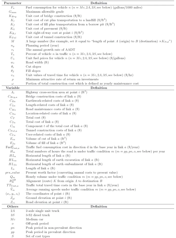
Table 3. Denitions of the parameters and the variables used in the model of this study.
Parameter Denition
Fn Fuel consumption for vehicle n (n = Mc; 2A; 3S; see below) (gallons/1000 miles) Gmax Maximum allowable grade
KBrg Unit cost of bridge construction ($/ft)
Kc Unit cost of cut plus transportation to a landll ($/ft3) Kf Unit cost of ll plus transportation from a borrow pit ($/ft3) KL Unit cost of pavement ($/ft)
KR;i Unit right-of-way cost at point i ($/ft2) KT nl Unit cost of tunnel construction ($/ft)
M A large number (for example, set it equal to \length of point A (origin) to B (destination) KT nl") ny Planning period (year)
rt The annual growth rate of AADT
Tn Percent of vehicle n in trac n (n = Mc; 2A; 3S; see below)
Un Unit fuel prices for vehicle n (n = Mc; 2A; 3S; see below) ($/gallons) wr Road width (ft)
c Cut slopes f Fill slopes
n Unit values of travel time for vehicle n (n = Mc; 2A; 3S; see below) ($/hr) Minimum attractive rate of return on investments
! Portion of total construction cost which is dened as yearly maintenance cost
Variable Denition
Ai Highway cross-section area at point i (ft2) CBrg;a Bridge construction costs of link a ($)
CEa Earthwork-related costs of link a ($) CLa Length-related costs of link a ($) CMa Road maintenance costs of link a ($) CNa Location-related costs of link a ($)
CT Total cost ($)
CT a Total cost of link a ($)
Cta Component t of the total cost of link a ($) CT nl;a Tunnel construction costs of link a ($)
CUa User-related costs of link a ($) Eca Volume of cut of link a (ft3) Efa Volume of ll of link a (ft3) Fueld
Cost;a Trac fuel consumption cost in direction d in the base year in link a ($/year)
Hm Total numbers of hours the road is under trac condition m (m = pp; pn; o; see below) per year HLa Horizontal length of link a (ft)
HLca Horizontal length of earth excavation of link a (ft) HLfa Horizontal length of earth embankment of link a (ft)
La Length of link a (ft)
prs value Present worth factor (converting annual costs to present value) Qm Hourly volume under trac condition m (m = pp; pn; o; see below) RAB
K Alignment (route) K from origin A to destination B
T TCost;a Trac total travel time costs in the base year in link a ($/year)
Vm Average running speeds under trac condition m (m = pp; pn; o; see below) (xi; yi; zi) The coordinates of point i (ft)
Zgi Ground elevation at point i (ft) Zri Road elevation at point i (ft)
Others Denition
2A 2-axle single unit truck 3S 3-S2 diesel truck Mc Medium car
o O-peak period
pn Peak period in non-prevalent direction pp Peak period in prevalent direction
(i) Using complementary concepts, such as Pareto optimality, in multi-objective analysis of the prob-lem [47,49] or sustainable development [47]; (ii) Employing additional techniques to improve
com-putational speed or alignment quality in genetic algorithms [1,48] and devising new hybrid search techniques [53,54], or new mixed integer pro-gramming procedures, to upgrade computational precision in earthworks [28,29];
(iii) Embedding complementary information systems, such as GIS, in the solution procedure [4,20, 36,38,51];
(iv) Incorporating important decisions for the choice of intersections, bridges, and tunnels into the alignment design [37,41].
Recent advances in this area add the vehicular fuel consumption and safety aspects to the alignment de-sign [56].
One important drawback of the existing path-nding algorithms is the rigidity of the procedures in adapting road alignments to the terrain at xed points along the line joining the two ends of the road (for example [55]). The proposed procedure in this paper is exible in this sense. It is able to maneuver around obstacles, land features, etc. by adding as many breaking points as required to pass smoothly through them. The designed test problems evaluate the maneuvering capabilities of the proposed algorithm.
One research direction in the eld of highway alignment design is to devise/discover methods to arrive at quality solutions eectively. This aspect of the solution methods will gain high importance soon in the light of the additional inertia that will be imposed on the methods by the features mentioned above. Proof of ingenuity of the procedures in arriving at quality solutions needs some test problems which are able to assert it. Such a set of test problems could serve as a basis for alternative method comparisons, in which corresponding researches are found to be very limited in the literature, particularly on a common basis (see, for example, Shaw and Howard [6], and Cheng and Jiang [57], in this respect.). The suggested test problems may form a platform for comparing future algorithmic developments and providing bench marks for dierent algorithmic performances.
3. The proposed solution procedure
The procedure employed to solve the road alignment problem has a meta-heuristic nature. To comply with the nature of such a procedure, it is run only over feasible solutions (routes). In doing so, constraints (such as maximum grade) are investigated for each candidate (newly found) alignment, and a large cost
(M) is added to the objective function of infeasible routes. Table 2 shows the transformed problem in this respect. Note that, in practice, we need not to bear the cost of objective function computations for infeasible alignments, as it is set equal to a large number, M.
The procedure used in this study to solve the 3D road alignment problem is an electromagnetism-like meta-heuristic algorithm (EA). This algorithm, introduced by Birbil and Fang [58], is notably dierent from other meta-heuristic algorithms as follows: they are not only local and global elites that inuence others (like particle swarm algorithm [59]), but so do all the particles. Moreover, particles not only exert attraction forces upon other particles, they repel other particles, too. While good solutions' elements are strengthened by pheromone addition and the other elements are weakened by pheromone evaporation (a size n operations) in algorithms such as ant system, in EA, we have a size n n operation of getting closer to all good elements and getting away from the inferior ones, proportional to the attraction/repulsion forces exerted upon them. In the former algorithm, all eective (ineective) alternatives are treated alike, while alternatives are given merits (demerits) in EA proportional to their attraction (repulsive) forces. The EA is more suitable for continuous variable uncon-strained optimization, and our 3D alignment problem may be dened in such an environment. The following review of EA provides us with the justication to use and prefer an adaptation of this algorithm to the other meta-heuristics.
The application of the electromagnetism-like al-gorithm has found its way into many areas of science and engineering. Examples include medical data classi-cation and prediction of diabetes mellitus [60], sensor distribution strategy to increase the coverage area of wireless sensor network after random distribution of sensors [61], machine-cell formation and layout problem in cellular manufacturing system in which parts with dierent characteristics and needs are assigned to the cells of distinctively divided machines [62], optimiza-tion of tool path planning in 5-axis CNC machining to reduce the geometrical deviations of the ruled surfaces [63], scheduling of the ow shop problem [64], and computation of numerical solutions to the inverse kinematic problem of robotic manipulator [65].
Moreover, EA has found applications in opera-tions research problems, too. Recent examples include traveling salesman problem with time windows [66], vehicle routing problem with delivery time cost [67], capacitated vehicle routing problem [68], and uncapac-itated multiple p-hub median problem [69]. Recent applications in transportation problems also include location and transportation planning in the supply chain problem [70].
electromagnetism-like algorithm has been found eective in solving sys-tem design problems in hybrid forms with other heuris-tic algorithms [62,64], meta-heurisheuris-tic algorithms such as Particle Swarm Optimization (PSO) [71], Simulated Annealing (SA) [64,67], as well as with conventional optimization methods [65] and in improved formats of EA algorithm [60,68].
What promotes the use of EA further in our prob-lem is the encouragement that is inspired by the higher performance of EA compared to the other counterparts, as reported in the literature. In the recent studies of the following authors, the electromagnetism-like algorithm has been found to be (in their words) superior to the common state-of-the-art methods [60], preferable to Particle Swarm Optimization (PSO) and Articial Bee Colony (ABC) [61], and signicantly better than the Genetic Algorithm (GA) [62]. EA is reported, also, to outperform Simulated Annealing (SA) and many well-recognized constructive heuristics as well as to yield more eective solutions than PSO [64]. Moreover, the following statements have been reported in some other studies regarding the EA: feasible and near-optimal results are generated within shorter computational times as compared to the test algorithms, including beam-ACO (Ant Colony Optimization), Compressed Annealing (CA), specically designed heuristics, and dynamic programming [66]. Furthermore, Yurtkuran and Emel [68] found EA to be giving promising results within acceptable computational times when compared to other novel meta-heuristics such as Tabu Search (TS), SA, GA, ACO, and PSO. In addition, accord-ing to Kratica [69], EA shows excellent performance (compared to GA) by reaching all the previously known optimal solutions on the instances studied in a reasonable time and has advantages over the compared meta-heuristics on large-scale instances.
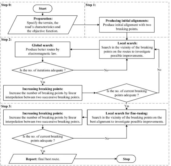
In what follows, an overview of the
electromagnetism-like algorithm is presented within the context of our problem. Highway alignment determination in a 3D space by the proposed algorithm is done in four macro-steps, as shown in Figure 1. In Step 0, the problem space is introduced to the procedure by dening the topography of the region, the two end points of the route, the objective function of the problem, and the constraints that should be observed when constructing the route. The forbidden area constraints have been introduced to the program by specifying extremely high land-acquisition cost for the right-of-way of the road in the forbidden region.
Step 1 of the macro-procedure is devoted to the generation of a set of random road alignments between the two end points, which together cover the region fairly well. In Step 2, an adaptation of the algorithm of Birbil and Fang [58] is applied to improve the current road alignments and to form a better set of alternative alignments. This algorithm is comprised
of two search routines: performing global and local searches. In the global search, by using Coulomb's law, the algorithm exerts the equivalent electrostatic forces on the particles (points along alignments) and changes the positions of the breaking points of the alignments, thus making new road alignments. In the local search, the algorithm changes the breaking points of the alignments randomly, with the hope of nding alignments with better values of the objective function. Our initial experiments with this algorithm have shown that increasing the global search iterations beyond a certain number does not change the bet-ter alignment found, and it is only the local search which reduces the objective function further. On the other hand, a great deal of computation time is spent to generate alignments with the higher number of breaking points and to compute the total cost of the new alignments. Thus, to increase the speed of the algorithm in concluding the nal result and avoid excessive ineective searches, Step 3 of the algorithm only conducts local searches around the better align-ment found in Step 2, without any global search. In the proposed algorithm, the initial alignments are built only with two breaking points. Steps 2 and 3 may increase these breaking points to form better alignments. The algorithm may also save computation time by holding the breaking points constant and move between consecutive steps.
4. The proposed algorithm
In this section, an electromagnetism-like meta-heuristic algorithm is proposed to nd and apply the solution of the 3D highway alignment design problem. Further descriptions of the original algorithm may be found in [58]. A pseudo-code of the algorithm, rst, is presented to bring the whole picture into the sight and, then, present a detailed version of the algorithm. 4.1. Pseudo-code of the proposed algorithm A pseudo-code of the proposed electromagnetism-like meta-heuristic algorithm for the solution of the 3D alignment problem, based on Figure 1, is as follows: 0. Preparation. Specify the inputs of the problem; 1. Initial alignments. Produce a pre-specied number
of two-breaking-points alignments; 2. Road alignment design:
2.1. Do while breaking points declared adequate; 2.2. Do while maximum iteration no. reached:
2.2.1. Local search. Search in the vicinity of the breaking points for improvements; 2.2.2. Global search. Produce better routes by
the electromagnetic law; Endo 2.2.
Figure 1. Basic structure of the electromagnetism-like model.
2.3. Raise the no. of breaking points. Increase the no. of breaking points by a linear interpolation between two successive breaking points; Endo 2.1.
3. Alignment ne tuning. Do while breaking points declared adequate:
3.1. Local search. Search in the vicinity of the breaking points for improvements;
3.2. Raise the no. of breaking points. Increase the no. of breaking points by linear interpolation between two successive breaking points; Endo 3.
Report the best alignment design specications. 4.2. Detailed description of the proposed
algorithm
The algorithm is described below:
Step 0. Determination of specications of the problem.
(a) Terrain. Specify the (x; y; z) coordinates of the points that dene the topology of the ground surface of the study area. Software, like Matlab, R2011b, may model the terrain by having the im-portant points and may estimate the elevation of any other point by linear interpolation between those points.
(b) Road. Specify the following alignment and design specications: the coordinates of the end points A : (xA; yA; zA) and B : (xB; yB; zB), the
max-imum allowable grade (Gmax), the road width
(wr), and the cut and ll slopes (c and f);
(c) Objective function. Determine the unit costs of the components of the objective function given in Eq. (1).
Step 1. Specication of the initial highway align-ments. Each specic alignment i of the road, Ri, is
represented by a matrix with three rows showing the (x; y; z) coordinates and the number of columns equal to that of the breaking points of the road plus two end points A and B. Thus, each column of this matrix represents the coordinates of a turning point on the
Figure 2. Selection of the space of the rst and second breaking points for the initial set of highway alignments.
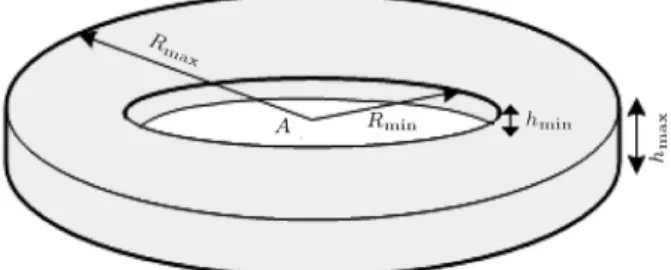
alignment under considerations. Generate m random alignments between A and B as follows. All initial alignments have two breaking points between A and B. For any such alignment, specify the breaking point next to A within a hollow cylinder around it, with internal radius Rmin, external radius Rmax, internal
height hmin, and external height hmax, as shown in
Figure 2.
The above-mentioned four parameters are de-termined as follows:
d=(xB xA)2+(yB yA)2+(zB zA)21=2; (2)
Rmin=d3; Rmax= 1:5Rmin;
hmin=Rmin Gmax; hmax=Rmax Gmax: (3)
Step 2. Global and local searches by the electro-magnetism-like algorithm.
(a) Model parameters. Specify the following model parameters:
zglobal The range of global search in the
vertical direction;
zlocal The range of local search in the vertical
direction;
x and yThe ranges of allowable search in the horizontal directions;
The coecient of local search in the horizontal directions;
# The exponent of the denominator of the Coulomb's Law;
BPmax The maximum number of breaking
points on the alignment;
GSIter The maximum number of Global Search Iterations;
LSIter The maximum number of Local Search Iterations.
Start local search. Local search is planned to investigate possible improvements of the align-ments in the vicinity of these routes. Such improvements may be identied by performing
the following operations. For each alignment, Ri,
a new alignment, Ri
new, is built.
(b) Replace the intermediate (breaking) points of the route (t = 2; 3; , and t 6= rst and last columns) with the following respective points:
Ri
1t new:= Ri1t+ (Rand 0:5)::x;
Ri
2t new:= Ri2t+ (Rand 0:5)::y;
Ri
3t new:= Ri3t+ (Rand 0:5):zlocal; (4)
where Ri
st is the (s; t) entry of matrix Ri (t =
breaking point; s = coordinate axis); in addition, we will have a new alignment matrix as follows:
Ri new=
2 4xA x
i
1new xi2new xB
yA yi1new y2newi yB
zA zi1new z2newi zB
3 5 ;
where Rand is a uniformly distributed random number in [0,1].
Cost computation. Compute the cost of the newly found alignment Ri
new. If the cost of Rinew
is less than Ri, save alignment Ri
new. If the
number of iterations is less than LSIter, go to Step 2(b); else, go to Step 2(c).
(c) Replace the incumbent alignment, Ri, by the
better solution of Ri
new (end of local search).
(d) Start the global search. Now, using the electromagnetic law, push alignment Ri away
from the worse alignments and bring it closer to the better ones. Sort all alignments Ri in the
order of increasing cost and identify the better one by Rbest.
(e) Electromagnetism. Compute virtual electromag-netism qi of alignment Ri as follows:
qi = exp mP f(Ri) f(Rbest) m
k=1(f(Rk) f(Rbest))
:
(5) (f) Electromagnetic force. Compute the electromag-netic force exerted on alignment Ri by alignment
Rj as follows:
Fji=
8 > > < > > :
(Rj Ri) qiqj
kRj Rik#; if f(Rj)<f(Ri)
(Ri Rj) qiqj
kRj Rik#; if f(Rj)f(Ri) (6)
and, thus, the resulting force is as follows: Fi=Xm
j6=i
Fji i = 1; 2; ; m: (7)
Fjiand Fiare both 3-row matrices with columns
(g) Alignment reformation. Move each breaking point of alignment Ri in the direction of the
force exerted on it by a step size , which is a uniformly distributed random variable at the interval of [0,1], as follows:
Ri st:= 8 > > > > > > > < > > > > > > > : Ri st+ F
i st
kFik
max
s Rist
Ri
st
; if 0 Fi
st
Ri st+ F
i st
kFik
Ri
st mins (Rist)
; if Fi
st< 0
s=1; 2; 3; i=1; ; m; i 6= best: (8) Herein, max
s ( ) and mins ( ) dene the boundaries
of the coordinate axes. In this process, the best alignment, Rbest, does not move from its place
and will be transferred to the next iteration of the algorithm in its original form.
(h) Cost computation. Compute the cost of the new alignments.
(i) Maximum iteration check. If the number of itera-tions equals GSIter, go to Step 2(j) to smooth out alignments; else, go to Step 2(b) for local search. (j) Start increasing breaking points. To increase the precision of the alignments and to decrease their costs, if the number of breaking points along the alignments is less than BPmax, increase the
number of breaking points along the alignments by linear interpolation between two successive original breaking points along these routes. Add these new breaking points to the alignments and go to Step 2(b) for local search, after reducing co-ecient of horizontal local search by half, i.e., setting := =2 in order to reduce the chance of the alignment intermingling in Step 2(b). Else if the number of the breaking points is greater than or equal to BPmax, go to Step 3 for local
ne-tuning of the best alignment found.
Step 3. Local search for ne-tuning the best align-ment.
(a) Set model parameters. Specify the following model's parameters for this step:
d
BPmax The maximum number of breaking
points on the alignment; c
LSIter The maximum number of local search iterations;
SubIter The maximum number of iterations for the local search sub-iteration.
Set local search iteration to q := 1 and the local search Sub-iteration to r := 1.
(b) Start local search. For alignment Rbest, build
a new alignment Rbest
new by replacing the
inter-mediate (breaking) points of the route with the respective points as computed in Eq. (4). Thus i is replaced by \best".
Cost computation. Compute the cost of the newly found alignment Rbest
new. If the cost of Rbestnew
is less than Rbest, save alignment Rbest
new. If r <
SubIter, set r := r + 1 and go to Step 3(b); else (if r SubIter) go to Step 3(c).
(c) Replace the incumbent alignment Rbest by the
better solution of Rbest
new (end of local search).
(d) Redo local search: If q < cLSIter, set q := q + 1, and go to Step 3(b); else (if q cLSIter) go to Step 3(e).
(e) Start increasing Rbest breaking points. If the
number of the breaking points along the align-ment is less than dBPmax, increase the number of
breaking points along Rbestalignment by linear
interpolation between the two successive original breaking points along this route. Add these new breaking points to the alignment and go to Step 3(b) for local search, after setting q := 1, r := 1, and := =2, else if the number of the breaking points is dBPmax, introduce Rbest as
the best route and stop.
5. Calibration of the proposed algorithm To calibrate the algorithm for an ecient and eective use, the model's parameters are classied into three groups:
(a) Various iteration limits;
(b) Parameters that follow certain rules; (c) Irregular parameters.
The rst group includes GSIter and LSIter in Step 2 as well as cLSIter and SubIter in Step 3. The number of the initial alignments, m, in Step 1 is also of this nature. It aects the computational complexity in Step 2. By running the algorithm, and nding that the best-found alignment (according to our objective function in Eq. (1)) remains the same, after several iterations, that iteration may be considered as GSIter. The increase in the iteration limits of the parameters in Group (a) would increase the precision of the results on the one hand, while increasing the computation time on the other hand.
Group (b) parameters follow certain available binding information. These parameters comprise the following: x, y, BPmax, and dBPmax. The rst two
two horizontal directions, may be dened as follows: x = max(x) min(x);
y = max(y) min(y): (9)
In other words, x and y show the dimensions of the terrain under study. The other two parameters, however, limit the maximum number of the breaking points along the alignment. Let P be the current number of the intermediate breaking points in an alignment. Then, this number turns to:
P := 2 P + 1; (10)
after nishing the next smoothing-out operation along the road alignment. An appropriate value for P is a function of the extent of barriers and obstructions encountered when joining the two endpoints of the road alignment by a straight line. Such obstructions include (boundaries of) mountains, valleys, forests, wet areas, etc. The turning points provide opportunities to bypass such obstructions. Figure 3 helps to describe this point better. It also shows how the number of the turning points increases in later iterations. BPmax is specied
based on the number of the turning points that allows bypassing obstruction smoothly in connecting the two end points of the route. dBPmaxis determined based on
the design criteria for the minimum distance between the two consecutive stations required to settle the alignment on the ground. Thus, the upper bound d
BPmax may be found by dividing the route length by
the minimum station distance. This value should be lower than that obtained by Eq. (10).
Finally, Group (c) contains irregular parameters that hardly follow certain rules and may dier from one problem/case to another. In our procedure, #, ,
zglobal, and zlocal fall into this group. Determining
appropriate values for these parameters may be done by sensitivity analyses.
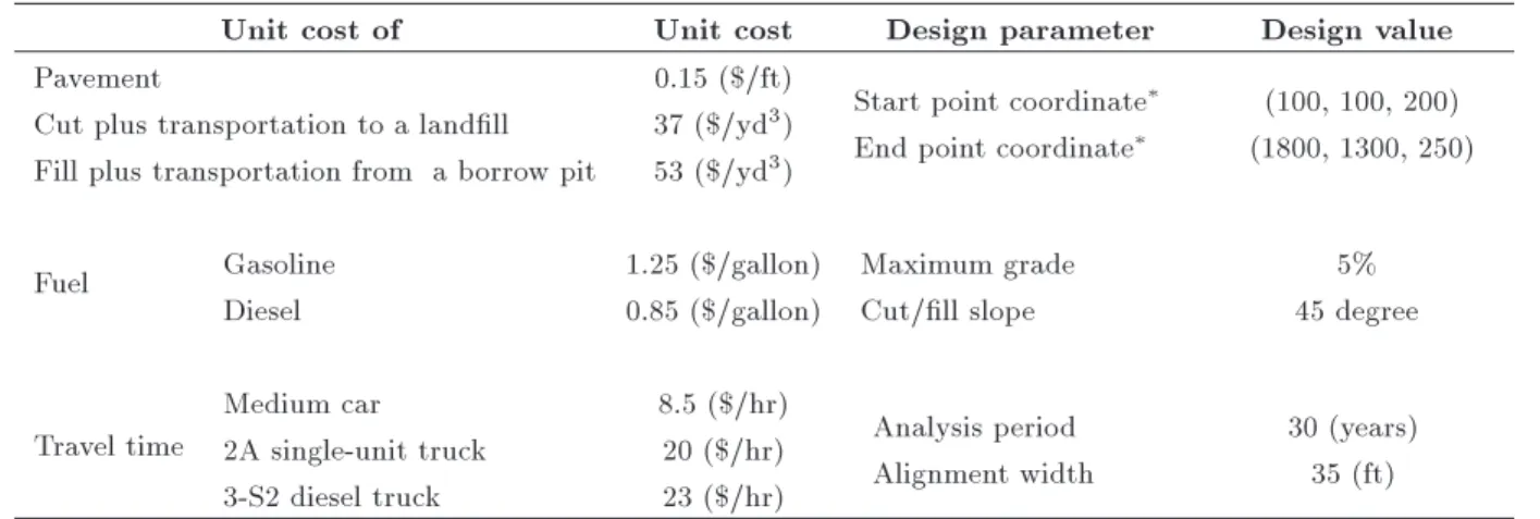
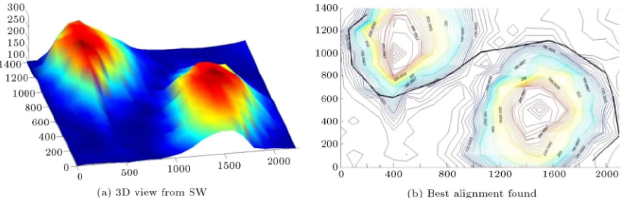
To calibrate our model, the case studied by Jha et al. [55] is employed for data availability reasons. The case comprises a terrain of 21001400 ft2. This terrain
is shown in Figure 4, both in 3D form and in contour lines. Table 4 presents the unit costs for this purpose and the specications of the alignment.
To use the model, it should be calibrated rst for better performance. Since there is insucient experience and data, if any, in this regard, we will resort to a heuristic procedure as follows, with the hope that the proposed model performs better than the un-calibrated model by choosing the better performing values for the parameters. It is notable that, at worst, we will work with an \inecient" algorithm. Then, the value of the most important parameter will be specied, and the value of that parameter of the model will vary within a reasonable range. To reduce the eect of non-calibrated parameters on the calibration of another parameter, the value of the parameter of concern within its range will vary, while the other parameters will be kept at their average (mid-range) value, or the best value found. It should be noted that the use of the average (mid-range) value of a variable with n possible equally likely values (because there is no information about their probability distribution at hand) would minimize the error of the choice. Computation of the value of the objective function in this one-dimensional search determines the value of that parameter, corresponding to the better value(s) of this function. To avoid the eect of the iteration number of the algorithm on the results, the number of iterations is held constant (herein, 20 for the sensitivity analysis on # and 10 for such analyses on , zlocal,
Figure 3. Increase of breaking points with the increase of barriers.
Table 4. Unit costs and design parameters used in this study for the reference problem obtained from Jha et al. [55].
Unit cost of Unit cost Design parameter Design value
Pavement 0.15 ($/ft)
Start point coordinate End point coordinate
(100, 100, 200) (1800, 1300, 250) Cut plus transportation to a landll 37 ($/yd3)
Fill plus transportation from a borrow pit 53 ($/yd3)
Fuel Gasoline 1.25 ($/gallon) Maximum grade 5%
Diesel 0.85 ($/gallon) Cut/ll slope 45 degree
Travel time
Medium car 8.5 ($/hr)
Analysis period Alignment width
30 (years) 35 (ft) 2A single-unit truck 20 ($/hr)
3-S2 diesel truck 23 ($/hr)
: The end points of the alignment are specic to our study, but are very close to those in Jha et al. [55].
Figure 5. Changes in the mean and the best cost obtained from 20 consecutive runs for dierent # with and without local search eect
and zglobal). To reduce the eect of the initial set
of alignments on the results, the algorithm is run many times (herein, 20), and the collective results are considered. The size of the initial set of alignments is chosen to be 20. The parameters are calibrated in the order and ranges of # 2 [0:5; 3:0] in Eq. (6), 2 [0:05; 0:5] in Eq. (4), zglobal 2 [0:25; 1:75] Z,
and zlocal 2 [0:01; 0:25] Z in Eq. (4), where
Z is max :fh; jzB zAjg, where h represents a
certain appropriate positive value. This order is a perceived order of importance, and the ranges are deemed reasonable based on the information found in the literature or perception. The calibration procedure pursued in this study is as follows:
Step 1. Specication of #: Parameter # relates to the global search and, hence, its value will be sought in two cases. First, Step 3 is omitted (of the local search), and LSIter (the maximum number of the local search iterations) is set equal to 1 (this would reduce the eect of the local search on the results to a minimum). Next, Step 3 is added to examine the joint eect of the local and global searches on the results. In all runs, the initial alignments are kept the same. Figure 5 shows that # = 1:0 is the better value
in both cases; however, the case with the local search step further reduces the minimum objective function; Step 2. Specication of zglobal, zlocal, and : To
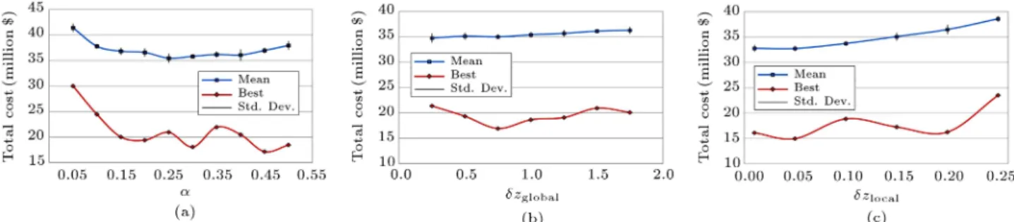
calibrate the model for these three parameters, the initial alignments and the generated random numbers may become eective. Hence, these two dimensions are considered by constructing ve sets of initial alignments; for each set, the program is run for 20 times. Then, the average (and, to some degree, the best) value of the objective function will indicate the most suitable parameter values as described below.
To specify , we set # = 1:0 (its best value), zglobal = 1:0, and zlocal = 0:13 (their respective
range average values). Figure 6(a) shows the best and average values of the objective function for the ve sets of alignments and for each given value of 2 [0:05; 0:5] in increments of 0.05. Considering the average value of the objective function over the 5 alignment sets and over the 20 iterations for each alignment set, a minimum value at = 0:25, where the minimum value of the objective function has also a good stance. Hence, = 0:25 is set.
To specify zglobal, # = 1:0, = 0:25 (their best
Figure 6. Changes in the mean and the best cost obtained from ve sets of initial alignments for three model parameters , zglobal, and zlocal.
Table 5. The pursued calibration procedure of the electromagnetism-like algorithm in this study. Order of
calibration
Parameter for calibration
Range of parameter
Other parameters' values assumed in the calibration
Calibrated parameter
# zglobal zlocal value
1 # [0:5; 3:0] 0.25 1.0 0.13 1.0
2 [0:05; 0:5] 1.0 1.0 0.13 0.25
3 zglobal [0:25; 1:75] Z 1.0 0.25 0.13 0.25
4 zlocal [0:01; 0:25] Z 1.0 0.25 0.25 0.05
set. Figure 6(b) shows the best and average values of the objective function for the ve sets of alignments and for each given value of zglobal 2 [0:25; 1:75] in
0.25 increments. It is evident in this gure that the average value of the objective function decreases and, then, stabilizes with the decrease of zglobal. Hence,
zglobal= 0:25 is chosen.
For zlocal, # = 1:0, = 0:25, and zglobal= 0:25
(at their best values) are set, and zlocal 2 [0:01; 0:25]
in 0.05 increments varies (except for the rst 0.04 increment). The variations of the average and best values of the objective function, due to the variation of zlocal in its range, are shown in Figure 6(c). It seems
in the gure that zlocal= 0:05 is a more suitable value.
Table 5 summarizes the calibration procedure for the algorithm and presents the results.
6. The performance of the algorithm
In what follows, the proposed algorithm is applied in the solution of several specically designed problems to show its performance. The English System of measurements (instead of the Metric System) is chosen because of the data at hand. Most unit costs have been borrowed from Jha et al. [55]. The program is coded in Matlab R2011b and run on a laptop computer with Intel Core 2 Duo 2.80 GHz CPU and 4.00 GB RAM. 6.1. Example 1. The shortest arrival distance Herein, we aim to nd the shortest path between the two points with the coordinates (800, 800, 200) and (2000, 2000, 300). The objective function is the
Figure 7. The shortest arrival distance (Example 1).
distance between these two points, and there is no constraint on the shortest path alignment.
Figure 7 shows 20 initial alignments and the shortest path (nally discovered). The shortest path between these two points has a length of 1700.0 ft, and it is also evident from this gure that none of the initial alignments is close to the shortest alignment. The results of 10 runs to solve the problem presented the shortest alignment lengths and the respective CPU times for nding them, as given in Table 6. The gures in this table indicate good precision and solution speed for this problem.
6.2. Example 2. The forbidden area problem The forbidden areas are places where passage of the road alignments through them is not allowed. They include forests, ponds, wet areas, and other reserved areas that have environmental, archaeological, or
simi-Table 6. Alignment distance and run times for Example 1.
Run Distance (ft) Run time (sec)
1 1700.47 1.919
2 1700.14 1.888
3 1701.83 1.872
4 1700.55 1.904
5 1700.64 1.904
6 1700.28 1.888
7 1700.89 1.903
8 1700.39 1.935
9 1700.01 1.919
10 1700.5 1.857
Min 1700.01 1.857
Mean 1700.57 1.8989
Max 1701.83 1.935
Std. Dev. 0.51 0.02
lar importance. In this example, an example terrain of 2100 1400 ft2 is constructed which includes a body
of water, as shown in Figure 8(a). In Examples 2 through 6, the unit costs of Table 4 and road mainte-nance cost of about 10% of the road construction cost are used.
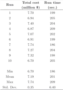
The road end points have coordinates (600, 1300) and (2000, 300) on the horizontal plane. Table 7 presents the results of 10 dierent runs to solve this problem, and the best alignment is shown in Fig-ure 8(b). It shows how the algorithm nds the best alignments to bypass the forbidden area between the two end points of the road.
6.3. Example 3. Flat area with several obstructions
The terrain in this example is more dicult to handle than that in Example 2, and the route has to wind through the area (Figure 9(a)). The two end points of the road have horizontal plane coordinates of (200,
Table 7. Total costs of the best-found alignments and the respective run times for Example 2.
Run Total cost (million $)
Run time (sec.)
1 7.70 199
2 6.94 205
3 7.40 204
4 6.87 209
5 7.07 202
6 6.91 199
7 7.74 186
8 7.27 204
9 7.32 198
10 6.70 205
Min 6.70 186
Mean 7.19 201
Max 7.74 209
Std. Dev. 0.35 6.40
1350) and (1900, 50). We do not allow building tunnels in constructing this route; therefore, it has to wind around the obstructions. The terrain in this example is of the same size as in Example 2 with dierent features in the topography. The results of 10 runs are presented in Table 8, and the best alignment is shown in Figure 9(b). This gure shows the capability of the algorithm to bypass the mountains. Moreover, based on Figure 9(b), the algorithm is able to move backward to nd a better alignment.
6.4. Example 4. Bridge construction
Bridges and tunnels may trade-o capital cost with road length-related costs: Higher construction costs with shorter roads. In Examples 4 through 6, the terrains are built ruggedly to promote the construction of roads with such facilities. Figure 10(a) and (b) show a terrain with a deep valley, and either of the two end points is located on either side of the valley
Figure 9. Flat area with several obstructions (Example 3). Table 8. Total costs of the best-found alignments and the
respective run times for Example 3. Run Total cost
(million $)
Run time (sec.)
1 13.74 301
2 12.51 264
3 13.71 260
4 13.45 258
5 15.39 299
6 16.87 254
7 13.28 266
8 13.35 268
9 13.28 244
10 13.81 280
Min 12.51 244
Mean 13.94 270
Max 16.87 301
Std. Dev. 1.26 18.68
with coordinates on the horizontal plane as (100, 400) and (1350, 300), so that the alignment between them needs to cross the valley axis line. This study assumes a bridge unit construction cost of 5000 $/ft (within certain specications regarding bridge length, valley depth, etc.). Table 9 presents the results of 10 runs of the algorithm for either case of when bridge construction is/is not possible. According to this table, in the case where bridge construction is possible, not only the total construction cost reduces, but also does the CPU computation time. The latter happens due to the relation between the computation eorts and the length of the alignment that reduces because of the bridge construction. Figure 10(c) and (d) show the best alignment of each of the two cases under considerations. It is interesting to compare the components of the total costs in the two cases, as shown in Table 10. The extra cost of the bridge construction is more than o-set by the reduction of all other cost components.
Table 9. Total costs of the best-found alignments and the respective run times for Example 4.
Without bridge With bridge Run
Total cost (million $)
Run time (sec.)
Total cost (million $)
Run time (sec.)
1 10.89 251 7.22 112
2 11.12 246 7.25 119
3 11.92 255 7.28 117
4 11.37 258 7.33 113
5 10.96 251 7.38 119
6 12.16 252 7.39 116
7 11.77 252 7.50 111
8 10.84 251 7.44 118
9 11.09 252 7.16 113
10 11.33 248 7.27 115
Min 10.84 246 7.16 111
Mean 11.35 252 7.32 115
Max 12.16 258 7.50 119
Std. Dev. 0.46 3.39 0.11 2.83
6.5. Example 5. Tunnel construction
Constructions of roads in mountainous terrains often require construction of tunnels. Figure 11(a) and (b) show a terrain designed for the purpose of this example, in which a high mountain obstructs the straight line alignment between the two end points of the route. The coordinates of these two points on the horizontal plane are assumed to be (200, 700) and (1800, 800). A tunnel unit construction cost of 3000 $/ft is assumed. Table 11 shows the results of 10 runs of the algorithm for two cases with/without tunnel construction. Once again, this table shows that the case with tunnel construction, as compared with the case of its alter-native under considerations, reduces both the total construction cost, as well as the CPU computation times, for the same reasons mentioned before for bridge
Figure 10. Bridge construction (Example 4). Table 10. The total cost break-downs for the best
alignment with/without bridge. Cost components
Best alignment cost (thousand $) Without
bridge
With bridge
Pavement 0.492 0.189
Earthworks 957 578
Fuel 607 233
Travel time 3212 1231
Bridge construction 0 1192
Right-of-way 1943 581
Maintenance 4123 3343
construction in Example 4. Figure 11(c) and (d) show the best alignment of each case under consideration. A component-wise comparison of the total costs of the two alignments in Table 12 indicates that the extra cost of tunnel construction is more than o-set by the reduction of all other cost components.
6.6. Example 6. A more general terrain
In this example, a more general terrain is made to show the performance of the proposed algorithm when more than one feature is present on the straight line alignment between its two end points. The end points are assumed to be at the coordinates (200, 2700) and
Table 11. Total costs of the best-found alignments and the respective run times for Example 5.
Without tunnel With tunnel Run
Total cost (million $)
Run time (sec.)
Total cost (million $)
Run time (sec.)
1 9.77 205 7.60 131
2 9.87 216 7.44 133
3 10.64 212 7.65 130
4 10.29 216 7.38 126
5 10.08 216 7.60 123
6 13.37 187 7.81 121
7 10.94 213 7.74 129
8 10.42 195 7.64 129
9 10.66 213 7.70 127
10 9.91 222 7.76 125
Min 9.77 187 7.38 121
Mean 10.60 210 7.63 127
Max 13.37 222 7.81 133
Std. Dev. 1.05 10.96 0.13 3.72
(4200, 2500) on the horizontal plane. The terrain consists of a dam (a body of water that may not be crossed) and a rugged area (Figure 12(a) and (b)), so that the alignment is better served by bridges and tunnels. In this example, the bridge and tunnel unit construction costs are assumed to be 5000 $/ft and
Figure 11. Tunnel construction (Example 5). Table 12. The total cost break-downs for the best
alignment with/without tunnel. Cost components
Best alignment cost (thousand $) Without
tunnel
With tunnel
Pavement 0.338 0.243
Earthworks 1600 340
Fuel 417 300
Travel time 2208 1588
Tunnel construction 0 1195
Right-of-way 1353 734
Maintenance 4197 3225
8000 $/ft, respectively. Table 13 shows the results of 10 runs of the algorithm for the solution of this problem. Figure 12(c) shows the best alignment among the 10 runs. It shows the use of the bridge on the deep valley and two tunnels to overcome the two high mountains on the sides.
6.7. Example 7. Solution to an existing problem
In this example, the performance of the proposed algorithm in this study will be shown on a test problem given by Jha et al. [55]. The terrain of the problem is shown in Figure 4. The unit costs and alignment specications, used in this comparison, are given in
Table 13. Total costs of the best-found alignments and the respective run times for Example 6.
Run Total cost (million $)
Run time (sec.)
1 33.01 444
2 34.50 467
3 34.48 506
4 33.72 512
5 37.02 518
6 35.29 408
7 33.33 434
8 34.50 544
9 38.03 475
10 37.87 505
Min 33.01 408
Mean 35.18 481
Max 38.03 544
Std. Dev. 1.84 42.94
Table 4, respectively. To have the results closer to the respective ones, given by Jha et al. [55], this study ignores maintenance cost in the cost computation, but considers the accident costs equivalent to 10% of the total cost of the alignment (according to the information given by Jha et al. [55]). Table 14 shows the results of three (10) runs of the proposed
Figure 12. A more general terrain (Example 6). Table 14. The results of three separate trials of the
algorithm in this study and those of Jha et al. [55] on the same problem (million $).
Run Trial 1 Trial 2 Trial 3 Jha et al. [55] 1 16.06 14.22 15.28 27.202 2 19.13 17.58 19.31 24.412 3 14.21 14.97 21.88 27.323 4 15.63 19.35 17.05 25.370 5 14.60 16.83 14.95 21.086 6 14.21 20.25 15.24 23.154 7 20.14 17.07 14.73 23.709 8 13.97 16.54 15.47 25.223 9 17.024 19.54 14.78 24.845 10 14.28 14.29 15.33 25.942 Min 13.97 14.22 14.73 21.086 Mean 15.93 17.06 16.40 24.827 Max 20.14 20.25 21.88 27.323 Std. Dev. 2.20 2.17 2.38 1.879
electromagnetism-like algorithm. This table shows that, in all of the three separate experiments, the proposed electromagnetism-like algorithm nds align-ments whose mean construction costs (for the 10 runs)
are very similar to each other. The best alignment among the three alignments is shown in Figure 13. It also shows how an increase in the number of the breaking points in our alignment design would aect the capability of the proposed algorithm in providing a more exible alignment to t the topography of the terrain. Table 14 also includes the values of the objective function for the 10 runs of the algorithm presented in Jha et al. [55]. It is to be noted that, although the objective functions of the two studies are basically the same, their alignment specications (constraints) dier in some respects (for example, in building the horizontal and vertical curves). This is why we lose ground for the comparisons of the two algorithms. In the passing process, based on Table 14, it is worth noting that our three trials result in higher standard deviations for the objective function values of the 10 solutions found in the dierent runs, as compared to the study result of Jha et al. [55]. This is because the algorithm of this study, unlike that of Jha et al. [55], does not constrain itself in the 3D space when searching for better alignments.
Figure 14 presents the break-down of the total cost of the nal route alignment in this example (Note that the pavement cost is low, not zero in this gure.).
Figure 13. The best alignment between end points A and B found by the algorithm for dierent breaking points in Example 7.
Figure 14. The shares of the major cost components for the best alignment in Example 7.
This gure shows that, based on the input data, three cost components of earth works (32%), users' travel time (28%), and right-of-way (26%) sum up to 86% of the alignment total cost.
7. Summary and conclusions
This paper presented an adaptation of the electromagnetism-like algorithm to solve the three-dimensional route alignment design between two points. The review of the literature in this area revealed that after a break-through progress from the two-dimensional alignment design algorithms to the three-dimensional ones, there was a potential for enhancing the quality of the 3D alignment design and embedding capabilities for deciding dierent trade-os between various cost components. More specically, such trade-os exist between road structural elements, like bridges and tunnels, and all other road length-related costs, like earthworks (cuts and lls) and the user's travel times.
For this purpose, an electromagnetism-like algo-rithm [58] was adapted to solve the 3D alignment design problem. Seven examples were devised to test the performance of the algorithm in terms of the algorithmic capabilities, design, and speed of solving the problem. The application of the algorithm in these examples showed satisfactory results.
The contributions of this study to the eld are as follows:
1. Introduction and adaptation of an ecient algo-rithm to solve the 3D alignment problem, which can:
(i) Consider the real-world cost components; (ii) Make a trade-o between cost components by
comparing more conventional wavy or zigzag routes with more modern structures to build more straight alignments;
(iii) Observe the constraints in the alignment de-sign, such as the maximum slopes and re-served/forbidden areas.
2. Implementation of the concept of breaking point mechanism within the algorithm, which grants the algorithm the necessary exibility to bypass obstructions more smoothly.
It is not possible to compare our algorithm with the existing algorithms due to the dierences in the objective functions as well as the constraints of the problems under study. Table 15 presents the specication of this study with those of a prominent algorithm in the 3D highway alignment problem. As is evident in this table, we think that maintenance cost is an important cost component to consider, and maximal allowable horizontal and vertical curvatures
Table 15. A comparison of the objective functions and constraints in this study and those of Jha et al. [55].
Items
Problem cost components in
the objective function Problem constraints
Lo cation-related Length-related Earth w ork-related Acciden t costs Bridge and tunnel construction Road main tenance T rac fuel
consumption Trac
total tra vel time Maximal allo w able gradien t Maximal allo w able curv ature for horizon tal alignmen t Maximal allo w able curv ature for vertica alignmen t
Overall This study X X X | X X X X X | |
Jha et al. [55] X X X X X | X X X X X
Example 7 This study X X X X | | X X X | |
Jha et al. [55] X X X X | | X X X X X
are detailed design-level, and not highway alignment-design-level, considerations. Such dierences prevent easy comparison of the performances of dierent algo-rithms. We hope that with the information provided in this study about the 7 test examples, there will be a common platform for such comparisons in the future. This will obviate the awkward and unnecessary task of the iterative computer coding of other involved procedures for comparison purposes in order to con-vince independent observers of the merits of the new algorithms.
Further study in this area may pay more at-tention to linking such algorithms with geographical information systems and its application to cases where sucient eorts have been made to arrive at nal alignments, which may serve for validation purposes. Acknowledgements
The authors would like to present their sincere appreci-ation to Leila Pourzahedi and Sabiheh-alsadat Faghih whose works paved the way for this study. We are also thankful to J. C. Jong who provided data to the latter author, used for our model calibration and performance exhibition. Finally, the authors would like to express their gratitude to the anonymous referees for their helpful comments that enhanced the content and the presentation of the paper.
References
1. Kim, E., Jha, M.K., and Son, B. \Improving the computational eciency of highway alignment opti-mization models through a stepwise genetic algorithms approach", Transportation Research Part B: Method-ological, 39(4), pp. 339-360 (2005).
2. Kang, M.-W., Jha, M.K., and Schonfeld, P.
\Appli-cability of highway alignment optimization models", Transportation Research Part C: Emerging Technolo-gies, 21(1), pp. 257-286 (2012).
3. Jong, J.-C. and Schonfeld, P. \An evolutionary model for simultaneously optimizing three-dimensional high-way alignments", Transportation Research Part B: Methodological, 37(2), pp. 107-128 (2003).
4. Jha, M.K. and Schonfeld, P. \A highway alignment optimization model using geographic information sys-tems", Transportation Research Part A: Policy and Practice, 38(6), pp. 455-481 (2004).
5. Howard, B., Bramnick, Z., and Shaw, J., Optimum Curvature Principle in Highway Routing, Road Re-search Laboratory/UK (1969).
6. Shaw, J.F. and Howard, B.E. \Comparison of two integration methods in transportation routing", Trans-portation Research Record, 806, pp. 8-13 (1981).
7. Shaw, J.F. and Howard, B.E. \Expressway route optimization by OCP", Transportation Engineering Journal, 108(3), pp. 227-243 (1982).
8. Thomson, N. and Sykes, J. \Route selection through a dynamic ice eld using the maximum princi-ple", Transportation Research Part B: Methodological, 22(5), pp. 339-356 (1988).
9. Wan, F., Introduction to the Calculus of Variations and its Applications, Boca Raton, Florida, United States CRC Press (1995).
10. Turner, A.K. and Miles, R.D., The GCARS System: A Computer-Assisted Method of Regional Route Location, West Lafayette, Indiana, United States Lafayette, in Purdue University (1971).
11. Athanassoulis, G. and Calogero, V. \Optimal location of a new highway from A to B-A computer technique for route planning", PTRC Seminar Proceedings on Cost Models & Optimization in Highway (1973).
12. Parker, N.A. \Rural highway route corridor selection", Transportation Planning and Technology, 3(4), pp. 247-256 (1977).