Sharif University of Technology
Scientia IranicaTransactions E: Industrial Engineering http://scientiairanica.sharif.edu
A class Hotelling model for sequential auctions of close
substitutes
E. Hu
a;b, C. Rao
c;, and Y. Zhao
aa. Systems Engineering Institute of Automation School, Huazhong University of Science and Technology, Wuhan 430074, P. R. China.
b. School of Science, Hubei University of Technology, Wuhan 430068, P. R. China. c. School of Science, Wuhan University of Technology, Wuhan 430070, P. R. China. Received 10 September 2016; accepted 26 May 2018
KEYWORDS Sequential auctions; Hotelling model; Supply chain; Associated valuation; Information policy.
Abstract. Against the background of supply chains, this paper constructs a class Hotelling model to describe and explore sequential auctions of close substitutes with slightly more general associated valuations. In this generalized model, both close substitutes and bidders are hypothetically distributed at the interval [0; 1], types of bidders are continuous, and each bidder's valuations for close substitutes are not independent. Moreover, with the aid of this model, equilibriums are explored, and eciencies of the auctions are analyzed under second-price sealed-bid auction formats. Further, considering two typical information policies, we investigate some concrete bids and revenues of the ecient sequential auctions, while bidders' valuations are linear functions of distances between them and close substitutes. Results show that eciencies of the sequential auctions are conditional, and inuences of information policies on revenues of the auctions are related to both numbers of bidders and locations of items.
© 2019 Sharif University of Technology. All rights reserved.
1. Introduction
In 1929, Hotelling developed a model of spatial compe-titions to demonstrate relationships between locations and pricing behaviors of rms through a line of xed length and predict an aggregation of two competing rms in the middle of the customers' support inter-val [1,2]. The standard Hotelling model assumes that all consumers are identical (except for locations) and evenly dispersed along the line; both the rms and consumers respond to changes in demand and the economic environment. As a game model, it can also be used to describe some auction problems in supply chains: m suppliers sell their supply contracts
*. Corresponding author.
E-mail address: [email protected] (C. Rao) doi: 10.24200/sci.2018.20546
sequentially or simultaneously to n agents with unit-demands via auctions, and both suppliers and agents are located in the same trac line. Here, suppliers and agents correspond to rms and customers, respectively. In addition, these contracts are deterministic and undierentiated for agents; thus, dierences among agents' valuations for contracts mainly depend on their transportation costs.
The above-mentioned problem can be abstracted as sequential auctions of close substitutes. Since the distance between an agent and his or her suppliers is considered, each agent's valuations for the suppliers' contracts are also considered, which are dierent from interdependent valuations among agents [3]. Hence, by means of the Hotelling model, our paper tries to focus on sequential auctions of close substitutes with slightly more general associated valuations. Here, key functions of close substitutes are the same or similar; however, their congurations or external performances
are slightly dierent so that various needs of consumers are met; thus, the private valuations of consumers are not exactly the same.
A key consideration of sequential auctions is a bidder's expected surplus for the follow-up auctions, which is usually concerned with future objects, bidder numbers, previous winning information, etc. Thus, information policy is always an important topic for auc-tions or other business activities, and theoretical and experimental studies have shown that revealing some information in advance will possibly aect the overall eciency and revenues of auctions [4,5]. Presently, there are major controversies and, consequently, a large body of literature about sequential auctions and information policies. Usually, while auctioned objects are heterogeneous and bidders' valuations are indepen-dent of each other, an expected revenue-maximizing auctioneer should fully and publicly reveal all infor-mation about auctioned objects [6-8]. However, while auctioned objects are homogeneous and bidders' valu-ations are not mutually independent, it was revealed that future objects or other related information in advance would uncertainly aect the overall eciency and revenues of sequential auctions [9-12]. Currently, in these pieces of literature, a bidder's valuations for homogeneous objects are usually supposed to be identical or proportional, which may be considered as especially associated valuations and lead to learning behaviors [13]. Owing to the diculty of modeling general associated valuations and processing mathe-matical expectations while a bidder type is multi-dimensional and continuous, existing researches mostly focus on sequential auctions where a bidder type is hypothetically discrete, namely H (High) or L (Low), and his or her valuations of objects are identical.
Recently, Zeithammer [14] studied sequential auc-tions of heterogeneous objects, discussed the inu-ence of revealing future objects on auction eciency and proved the existence of symmetric equilibriums and pure bidding strategies. Bayesian methods and the models used for processing a multi-dimensional continuous type in his paper inspired our studies. Accordingly, combined with characteristics of sup-ply chains, this paper explores the class Hotelling model for describing sequential auctions with some particular assumptions under second-price sealed-bid auction mechanisms. In the proposed model of the current study, both close substitutes and bidders are hypothetically distributed at the interval [0; 1]; a bidder type is continuous and multi-dimensional (namely, each bidder has dierent valuations for each close substi-tute); each bidder's valuations for close substitutes are not independent. Moreover, this model can skillfully convert multi-dimensional types into one-dimensional types via interdependence of distances between bidders and items in [0; 1].
The rest of this paper is organized as follows: Section 2 states formally the sequential auctions of close substitutes with associated valuations and con-structs a class Hotelling model. Section 3 proves the existence of equilibrium bids based on the model under the second-price sealed-bid auction format and explores some conditions of ecient auctions. Further, infor-mation policies, equilibrium bids, and overall revenues of the sequential auctions of close substitutes with especially associated valuations are specically deduced and discussed in Section 4. Relevant conclusions are summarized in Section 5.
2. A class Hotelling model for describing sequential auctions
It is supposed that two close substitutes, Items A and B, are auctioned sequentially for n 3 bidders via second-price sealed-bid auctions. Auction rules and some assumptions are as follows:
1. Item A is sold at the rst auction, and Item B is sold at the second one. In addition, at each auction, the bidder with the highest bid wins and pays the second highest bid. A tie is broken by rolling a fair coin;
2. Each bidder is risk neutral and has a unit-demand; accordingly, the bidder with Item A will exit the second auction;
3. Both items and bidders are distributed at the inter-val [0; 1] and mutually stochastically independent, as Figure 1 shows. The location of each bidder is his or her private information;
4. Each bidder's valuation for Item k 2 fA; Bg is Vk
(dk), where (dk) 0, 0(dk) > 0, and dk denotes
the distance between the bidder and Item k. Here, the value of Item k 2 fA; Bg, Vk 1 is commonly
known.
The last assumption is inspired by the standard Hotelling model [15]. When making trades in real-life markets, it is imperative to consider the factor of cost in general and its various types such as transportation costs or maintenance costs, which usually increase the functions of transportation distances. In this paper, Vk
is the same for all bidders. However, when taking into account transportation cost (dk), each bidder's true
valuation for k 2 fA; Bg should be Vk (dk), which
is dierent from those of other bidders.
Figure 1 shows the class Hotelling model. In Figure 1, the locations of Items A and B are denoted by 2 [0; 1] and 2 [0; 1], respectively. Without loss
of generality, it is assumed that . The location of a bidder at the interval is denoted by t 2 [0; 1]. To simplify the expressions, Bidder t is used to denote the bidder whose location in [0; 1] is t. Thus, the distance between Bidder t and Item A is dA(t) = j tj, and
one between Bidder t and Item B is dB(t) = j tj.
Accordingly, vk(t) = Vk (dk(t))(k 2 fA; Bg) is
Bidder t's valuation for Item k 2 fA; Bg. Furthermore, let bk(t) represent Bidder t's bid for k 2 fA; Bg.
Remark 1. In Figure 1, items and bidders corre-spond to rms and customers in the standard Hotelling model, respectively. While VA= VB, = 0 means
that the close substitutes (Items A and B) are identical for bidders, and = 1 means that maximum dierences exist among them. Moreover, similar to the preferences in the standard Hotelling model, the smaller the distance dk(t)(k 2 fA; Bg) is, the greater
Bidder t's valuation for item k will be.
Remark 2. In Figure 1, bidders' valuations for two items are their own private information and indepen-dent among bidders; however, each bidder's private valuations for two items vA(t) = VA (dA(t)) and
vB(t) = VB (dB(t)) are correlated because either
jdA(t) dB(t)j = or dA(t) + dB(t) = ,
while and are given in advance. Thus, the model in Figure 1 can be used approximatively to describe sequential auctions of close substitutes with particular assumptions of non-independent valuations, under which the probability of Bidder t winning Item B is intuitively relevant to one of his or her winning A. Concurrently, by means of t, our model skillfully converts a two-dimensional type of a bidder into a one-dimensional one. Thus, t may be also regarded as the bidder type.
3. Equilibrium and winners
Because the second stage of the sequential auctions in this paper is actually a private-value second-price sealed-bid auction, Bidder t's dominant strategy for Item B is to bid his or her own valuation for Item B, namely bB(t) = vB(t). However, deciding the bid
for Item A is more complicated than that for Item B, because Bidder t will consider his or her expected surplus in the second stage.
Let: x = max
6=t bA();
be the highest bid of Bidder t's n 1 opponents in the rst stage. If bA(t) > x, then Bidder t wins at the rst
auction and his or her surplus is vA(t) x. If bA(t) < x,
then Bidder t loses at the rst auction and all his or her remaining opponents at the second auction belong to (x) = ft0jb
A(t0) xg, which is a set of bidders whose
bids for Item A are not more than x. Further, let: n 2= t(z; (x)) = P ( max
2(x) and 6=tvB() z);
be the probability distribution function of the highest valuation of the remaining bidders (except t) at the second auction. Then, Bidder t 2 (x) can win Item B with a probability of n 2= t(vB(t); (x)), and his
expected surplus at the second auction is as follows: (vB(t); x) =
vZB(t)
0
(vB(t) z)dn 2= t(z; (x)): (1)
Obviously, winning Item A is more benecial to t if and only if vA(t) x > (vB(t); x). In addition, a
logical and ideal bid bA(t) should satisfy vA(t) bA(t) =
(vB(t); bA(t)) so that it would not make any dierence
for Bidder t to win Item A or to win Item B. In addition, because vA(t) (vB(t); 0) implies that
giving up Item A is always a good choice for Bidder t even though all other bidders bid 0 or do not submit their bids at the rst auction, it is assumed here that vA(t) > (vB(t); 0) holds for 8 t 2 [0; 1] in this
paper. Inspired by Zeithammer [14], Proposition 1 gives necessary and sucient conditions of equilibrium bid bA(t).
Proposition 1. Suppose that vA(t) > (vB(t); 0) for
8t 2 [0; 1). If and only if 1 + @(vB(t);x)
@x > 0 for
8t 2 [0; 1], there is a unique equilibrium bid bA(t) that
satises the following equation:
bA(t) = vA(t) (vB(t); bA(t)): (2)
Proof. Let S(x) = vA(t) x (vB(t); x).
Proposi-tion 1 needs to be proved based on the following two aspects:
1. S(x) = 0 has a unique solution, x0> 0, if and only
if 1 +@(vB(t);x)
@x > 0 for 8 t 2 [0; 1];
2. x0> 0 is Bidder t's equilibrium bid for Item A.
The solution under this condition can be divided into the following two cases to discuss:
i. If 1+@(vB(t);x)
@x > 0, then S0(x) = 1 @(v@xB(t);x) <
0. Therefore, S(x) strictly monotonically decreases with x. According to vA(t) > (vB(t); 0) for 8 t 2
[0; 1), we have S(0) > 0. Moreover, S(vA(t)) =
vA(t) vA(t) (vB(t); vA(t)) 0. Because
S(x) is continuous and strictly monotonic with x, there must exist a unique solution x0 2 (0; vA(t)]
satisfying S(x0) = 0.
Suppose that 1 +@(vB(t);x)
@x 0, then S0(x) =
1 @(vB(t);x)
@x 0. For instance, S(x)
S(x) S(0) = vA(t) (vB(t); 0) > 0, which
conicts with the condition that S(x) = 0 has one positive solution: x0 > 0. Thus, 1 + @(v@xB(t);x) >
0;
ii. It is assumed that bA(t) < x0. While bA(t) <
x0 < x = max6=t(bA()) or x < bA(t) < x0,
Bidder t is indierent to bid x0 or bA(t). While
bA(t) < x < x0, Bidder t will lose Item A
and his expected surplus at the second auction is (vB(t); x). Notice that S(x) > S(x0) = 0
because S(x) strictly monotonically decreases with x < x0. Accordingly, (vB(t); x) < vA(t) x.
Notice that vA(t) x is Bidder t's surplus if he or
she bids x0 and wins Item A. Therefore, bidding
bA(t) < x0 is worse than bidding x0 for Bidder
t.
A similar proof shows that bidding bA(t) > x0is worse
for Bidder t. Therefore, bA(t) = x0 is Bidder t's
equilibrium bid for Item A.
Remark 3. Essentially, 1 + @(vB(t);x)
@x > 0 is the
sucient and necessary condition of vA(t) (vB(t); x)
that has a xed point, which is Bidder t's equilibrium bid for Item A. Here, vA(t) bA(t) and (vB(t); bA(t))
are Bidder t's expected surplus at the rst auction and that at the second auction, respectively. Accordingly, Proposition 1 implies that winning Item A or B should yield the same expected surplus for Bidder t while he or she determines the optimal bid for Item A. Intuitively, Proposition 1 is also appropriate for sequential auctions of more than two items while Item A is regarded as the current item and Item B as the sum of all follow-up (or future) items.
Based on Proposition 1, Propositions 2 and 3 identify the winner at the rst auction.
Proposition 2. If (dk)(k 2 fA; Bg) is a linear
function of dk, 0(dk) > 0, and 1 +@(v@xB(t);x) > 0, then
Bidder t = arg min
t1;t2; ;tndA(ti) = arg mint1;t2; ;tnjti j
will win Item A.
Proof. Proposition 1 indicates that if 1+@(vB(t);x)
@x >
0, then equilibrium bid bA(t) for Item A is an implicit
function satisfying Eq. (2). According to vA(t) = VA
(dA(t)) and vB(t) = VB (dB(t)), we have:
dbA(t)
ddA(t) =
dvA(t)
ddA(t)
@(vB(t); bA(t))
@vB(t)
dvB(t)
ddA(t)
@(vB(t); bA(t))
@bA(t)
dbA(t)
ddA(t):
Namely:
dbA(t)
ddA(t) =
d(dA(t))
ddA(t) +
@(vB(t); bA(t))
@vB(t)
d(dddB(t))
B(t)
ddB(t)
ddA(t)
1 +@(vB(t); bA(t)) @bA(t)
1
= w
1 +@(v@vB(t); bA(t))
B(t)
ddB(t)
ddA(t)
1 +@(vB@b(t); bA(t))
A(t)
1
: (3)
In Eq. (3), w = d(dA(t))
ddA(t) =
d(dB(t))
ddB(t) > 0 because
(dk)(k 2 fA; Bg) is a linear function of dk and
0(d
k) > 0. Moreover, obviously:
@(vB(t); bA(t))
@vB(t) = n 2= t(vB(t); (bA(t))) 1;
and:
1 +@(vB@b(t); bA(t))
A(t) > 0:
If < t, then dB(t) = t = (t )
( ) = dA(t) ( ); if t < , then
dB(t) = t = ( ) (t ) = ( ) dA(t);
if t < < , then dB(t) = t = ( ) +
( t) = ( ) + dA(t). Accordingly, ddddBA(t)(t) = 1.
Thus,dbA(t)
ddA(t) 0, that is, bA(t) is a decreasing function
of dA(t) and an increasing function of vA(t) = VA
(dA(t)). Therefore, Bidder t nearest to Item A (i.e.,
t = arg min
t1;t2;tndA(ti) = arg mint1;t2;tnjti j) will win
Item A at the rst auction.
As a direct result of Proposition 2, the following corollary is obtained.
Corollary 1. The auction for Item A is ecient, while (dk)(k 2 fA; Bg) is linear, 0(dk) > 0, and
1 + @(vB(t);b)
@b > 0.
While (dk)(k 2 fA; Bg) is a non-linear function
of dk, which is contingent on predicting the winner at
the rst auction in advance. For example, let (dk) =
1 e dk and 8t > = 0, namely all bidders are
on the right-hand side of Item B in Figure 1. Then: dA(t) = t; dB(t) = t ;
and: dbA(t)
ddA (t) =
dbA(t)
= e t 1 + e
n 2= t(vB(t); (bA(t)))
1 + @(v@bB(t); bA(t))
A(t)
1
: If is large enough, then dbA(t)
ddA(t) or
dbA(t)
dt may be
more than zero, which means that bA(t) may be an
increasing function of dA(t) or t. However, vA(t) =
VA (dA(t)) = VA 1 + e dA(t) = VA 1 + e t
is a decreasing function of dA(t) or t. Therefore, the
auction for Item A may be inecient. Proposition 3. If 0(d
k) 0, 00(dk) 0, k 2
fA; Bg, 1 +@(vB(t);x)
@x > 0, and ti (i = 1; 2; ; n),
then Bidder t = arg min
t1;t2;tndA(ti) = arg mint1;t2;tnjti
j will win Item A.
Proof. Notice that ti (i = 1; 2; ; n) means
that all bidders on the right-hand side of Item A in [0; 1]. According to Proposition 1, Bidder t's equilib-rium bid is bA(t) = vA(t) (vB(t); bA(t)). Because
vA(t) = VA (dA(t)) and vB(t) = VB (dB(t)), we
have: dbA(t)
ddA(t) =
d(dA(t))
ddA(t) +
@(vB(t); bA(t))
@vB(t)
d(dB(t)) ddB(t)
ddB(t)
ddA(t) 1 +
@(vB(t); bA(t))
@bA(t)
1 : (4) Notice that:
@(vB(t); bA(t))
@vB(t) = n 2= t(vB(t); (bA(t))) 1;
and:
1 +@(vB@b(t); bA(t))
A(t) > 0:
If t , then dB(t) = t = dA(t) ( ) dA(t)
(* t ) and . Accordingly, ddB(t)
ddA(t) = 1 and
d(dA(t))
ddA(t)
d(dB(t))
ddB(t) 0 (*
0(dk) 0, 00(dk) 0 and
k 2 fA; Bg). Hence, dbA(t)
ddA(t) 0.
If t < , then dB(t) = t = ( ) dA(t) 0
(* t = 0 and ). Accordingly, ddB(t)
ddA(t) = 1. In
addition d(dB(t))
ddB(t) 0 and
d(dA(t))
ddA(t) 0 (*
0(d k) 0,
k 2 fA; Bg). Hence, dbA(t)
ddA(t) 0.
As a result, bA(t) is a decreasing function of dA(t)
or t. Therefore, Bidder t nearest to Item A (i.e., t = arg min
t1;t2; ;tndA(ti) = arg mint1;t2; ;tnjti j) will submit
the highest bid and win Item A.
Proposition 3 actually gives nonlinear conditions of ecient auctions in the class Hotelling model. Con-currently, its proof implies the following corollary.
Corollary 2. Let , 0(d
k) 0, k 2 fA; Bg, and
1 +@(vB(t);x)
@x > 0. The auction for Item A is ecient
while any one of the following conditions is satised:
1. 00(dk) 0 and ti (i = 1; 2; ; n); all bidders
are on the right-hand side of Item A;
2. 00(d
k) < 0 and ti (i = 1; 2; ; n); all bidders
are on the left-hand side of Item B;
3. All bidders are between A and B;
4. (dk) is linear, and Bidders' locations are arbitrary
in [0; 1].
Remark 4. Corollary 2 shows that the eciency of the sequential auctions described by the class Hotelling model is conditional. More specically, locations of suppliers and agents in a trac line should be considered for the auctions of supply contracts in Section 1.
4. Bids and information policies about The key to determining the equilibrium bid bA(t) =
vA(t) (vB(t); bA(t)) in Proposition 1 is the expected
surplus:
(vB(t); bA(t)) =
Z vB(t)
0 (vB(t) z)
dn 2= t(z; (bA(t)));
in which both vB(t) and n 2= t(z; (bA(t))) are
closely related to the location of Item B. Thus, in order to obtain a concrete formula of (vB(t); bA(t)), we
need to consider information policies about 2 [0; 1], namely revealing Item B or hiding Item B before the auction of Item A ends. Here, revealing Item B means that all bidders know , and hiding Item B means that all bidders do not know until the rst auction ends. In this section, we will apply the class Hotelling model to deduce some concrete equilibrium bids of sequential auctions of close substitutes.
Intuitively, any bidder at auctions subjectively regards himself or herself as a marginal loser [12] or winner, because he or she will rationally give up auctions if he or she nds no opportunities to win. Here, a marginal loser or winner respectively points to the loser with the highest bid or the winner with the lowest bid. Specically, in our class Hotellling model with (dk) = dk, the bidder nearest to Item A will
win according to Proposition 2 or Proposition 3. Thus, Bidder t regarding himself or herself as a marginal loser or winner of Item A always believes that the rest of his or her opponents are distributed on his right side (namely in [t; 1]), except none of his opponents dis-tributed in [0; t). Such an idea of a preponderant rival exactly leads to the bidding equilibrium mentioned by Proposition 1. For convenience, Bidder t is called a
preponderant rival of Item A if and only if there is at most one opponent in [0; t).
In order to facilitate discussions, it is assumed in this section that:
1. VA= 1 and VB = 1;
2. = 0 and (dk) = dk for k 2 fA; Bg.
The above assumptions imply that all bidders are on the right-hand side of Item A, namely t = 0, and (dk) is linear. Furthermore, let f(x) (F (x)) and
g(x) (G(x)) denote the probability density (probability distribution) of t and one of , respectively.
By means of Proposition 1 and Corollary 2, we will deduce the expected surplus (vB(t); bA(t)) of
Bidder t as a preponderant rival and verify and prove that bA(t) = vA(t) (vB(t); bA(t)) is exactly his or her
equilibrium bid for Item A.
4.1. Equilibrium bids when revealing
Each bidder knows Item A' location = 0, Item B's location 2 [0; 1], his or her own location (or type) t 2 [0; 1], and bidders' number n and does not know the locations (or types) of other bidders. However, he or she regards other bidders' locations as random variables distributed in [0; 1]. First, all n bidders submit their sealed bids for Item A. Then, the bidder with the highest bid wins Item A, pays the second highest bid, and exits the second auction. Next, the remaining n 1 bidders submit their sealed bids for Item B. Finally, the bidder with the highest bid wins Item B and pays the second highest bid.
First, let y
x(vB(t)) denote Bidder t's expected
surplus of winning Item B while he or she faces a group of opponents distributed at the interval [x; y], where x; y 2 [0; 1] and x y. According to Proposition 2, a preponderant rival of Item A can only defeat the bidders who are far away from Item A. Obviously, the probability density of the location of an opponent in [t; 1] is 1 F (t)f(s) , in which s 2 [t; 1]. Thus, the probability and the probability density that all locations of n 2 opponents in [t; 1] are greater than s 2 [t; 1] should be1 F (s)1 F (t)n 2and n 2
1 F (t)
1 F (s) 1 F (t)
n 3
, respectively. Therefore, while Bidder t only considers opponents on his or her right side, his or her expected surplus of winning Item B should be:
y
x(vB(t)) =
Z y
x
n 2 1 F (t)
1 F (s) 1 F (t)
n 3
(vB(t) vB(s))ds;
where t x y 1.
Then, in order to determine the expected surplus (vB(t); bA(t)) of Bidder t as a preponderant rival of
Item A in Figure 2, the interval [0; 1] is divided into
Figure 2. The case of W2.
three subintervals, namely W 1 = [0; t], W 2 = [t; (1 + t)=2], and W 3 = [(1 + t)=2; 1]. Thus, three cases need to be considered for .
Figure 2 shows the case of W 2. By observ-ing Figure 2, the optimal solution t of Eq. (2)
denotes the symmetric of t in [0; 1] with respect to , namely t = 2 t. Obviously, bids of
opponents in [t; t] for Item B should be greater
than one of Bidder t. Again, because opponents are distributed in [0; 1], (vB(t); bA(t)) is only
rel-evant to the opponents in [0; t] and [t; 1]. As a
preponderant rival of Item A, Bidder t subjectively believes that his or her n 2 opponents in the sec-ond stage should be distributed on his or her right side, namely in [t; 1]. Therefore, (vB(t); bA(t)) =
1
t(vB(t)). In addition, the other cases can be inferred
similarly.
Finally, a concrete formula of (vB(t); bA(t)) is
related to the specic probability distribution of t and one of . Further, it is assumed in Section 4 that t and are uniformly distributed in [0; 1].
To be specic, f(x) = 1, g(x) = 1, F (x) = x, and G(x) = x while x 2 [0; 1]. In conclusion, the expected surplus (vB(t); bA(t)) in various cases is
shown below.
1) 2 W 1:
(vB(t); bA(t)) = 1t(vB(t))
=
1
Z
t
n 2 1 F (t)
1 F (s) 1 F (t)
n 3
(s t)ds = n 11 t: (5)
2) 2 W 2 :
(vB(t); bA(t)) = 12 t(vB(t))
=
1
Z
2 t
n 2 1 F (t)
1 F (s) 1 F (t)
n 3
(t + s 2)ds
= (n 1)(1 t)(1 2 + t)n 1n 2: (6)
3) 2 W 3 :
(vB(t); bA(t)) = 0: (7)
Proposition 4. If is revealed before auctioning Item A, then Bidder t's equilibrium bid for Item A is bA(t) = 1 t (vB(t); bA(t)), where (vB(t); bA(t))
Proof. Let x = bA(tx) = max6=t bA() be the highest
bid of Bidder t's n 1 opponents in the rst stage and h(x) denote the probability density of x. Usually, equi-librium bid bA(t) should maximize Bidder t's expected
surplus (bA(t)) at the rst auction, namely:
max
bA(t)(bA(t)) = maxbA(t)
0 B @
bZA(t)
0
(VA(t) x)h(x)dx
+
1
Z
bA(t)
(VB(t); x)h(x)dx
1 C
A : (8)
Let: d(bA(t))
dbA(t) = (VA(t) bA(t))h(bA(t))
(VB(t); bA(t))h(bA(t)) = 0;
then:
VA(t) bA(t) (VB(t); bA(t)) = 0:
Hence, according to Proposition 1, we have 1 +
@(vB(t);x)
@x > 0. Again, on the base of Corollary 2,
x bA(t) in Eq. (8) means tx t. Moreover,
tx 1 for 8 2 (x) = fjbA() xg while
x bA(t).
) n 2= t(z; (x)) = P
max
2(x) and 6=tvB() z
= (P (vB() z while 2 (x)
= fjbA() x:g and tx 1))n 2
= R1
1+ zR f()d 1
txf()d
!n 2
=
z 1 tx
n 2
; where z VB(1) = 1 (1 ) = and f() = 1 in
[0; 1].
Next, we discuss the expected surplus in various cases as follows:
1. 2 W 1: (vB(t); x) =
vZB(t)
0
(vB(t) z)dn 2= t(z; (x))
=
1+ tZ
(1+ t z)(n 2)1 t
x
z 1 tx
n 3
dz
= (1 t)n 1
(n 1)(1 tx)n 2:
According to Corollary 2, x = bA(t) means tx = t.
Hence, (vB(t); bA(t)) = n 11 t;
2. 2 W 2: (vB(t); x) =
vZB(t)
0
(vB(t) z)dn 2= t(z; (x))
=
1 +tZ
(1 +t z)(n 2) 1 tx
z 1 tx
n 3 dz
=(n 1)(1 t(1 2 + t)n 1
x)n 2:
Hence:
(vB(t); bA(t)) = (1 2 + t) n 1
(n 1)(1 t)n 2:
3. 2 W 3: (1+t)=2 means vB(t) = 1 +t .
Then:
(vB(t); x)=
Z vB(t)
(vB(t) z)
dn 2= t(z; (x)) = 0:
Hence:
(vB(t); bA(t)) = 0:
Therefore, Bidder t's equilibrium bid for Item A should be bA(t) = 1 t (vB(t); bA(t)), where (vB(t); bA(t))
is shown as in Eqs. (5), (6), and (7). It is also easy to verify dbA(t)
dt < 0 through
Eqs. (5), (6), and (7). Thus, Item A will be allocated to the bidder with the highest valuation, namely one closest to A.
Remark 5. Eqs. (5), (6), and (7) imply that Bidder t = 1 or t 2 1 always bids his or her true valuation in the rst stage because he or she as a preponderant rival of Item A believes in advance that his or her expected surplus of winning Item B will be 0. However, Bidders t = 0 always hide their surplus
(1 2 maxf;1=2g)n 1
(n 1) in the rst stage by making use of
the advantage of their location.
4.2. Equilibrium bids when hiding
Item B (namely ) is hidden before the end of auction-ing A. Each bidder knows = 0, his or her own location (or type) t, and bidders' number n and does not know and other bidders' locations (or types). However, he or she regards other bidders' locations as random variables distributed in [0; 1], and believes that Item B is also distributed in [0; 1]. Similar to Section 4.1, the
key to determining the equilibrium bid is the expected surplus of winning Item B.
While is regarded as a random variable, Bidder t's expected surplus of winning B is (; b0
A(t)) =
E[(vB(t); bA(t))], and Bidder t's equilibrium bid for
Item A should be b0
A(t) = vA(t) (; b0A(t)). Hence:
(;b0
A(t)) = E[(vB(t); bA(t))]
=
t
Z
0
(vB(t); bA(t))g()d = t
Z
0
1 t
n 1d
+
1+t 2
Z
t
(1 2 + t)n 1
(n 1)(1 t)n 2d
=(1 t)(1 + (2n 1)t)
2n(n 1) : (9)
Proposition 5. If is hidden before the end of auctioning Item A, then Bidder t's equilibrium bid for Item A is b0
A(t) = 1 t (; b0A(t)), where (; b0A(t))
is introduced in Eq. (9).
Proof of Proposition 5 is similar to that of Propo-sition 4. Further:
db0 A(t) dt = d dt 1 t
1+2(n 1)t (2n 1)t2
2n(n 1)
=2 nn 1 < 0(* n 3): Thus, b0
A(t) is monotonically decreasing with t, which is
consistent with Proposition 2. Concurrently, db0A(t)
dt <
0 also indicates that Item A will be allocated to the bidder with the highest valuation, namely one closest to Item A.
Remark 6. According to Eq. (9), (; b0
A(0)) = 1
2n(n 1), (; b0A(0:5)) = 8n(n 1)2n+1 , and (; b0A(1)) = 0.
It can easily be proved that (; b0
A(t)) reaches the
maximum n
2(n 1)(2n 1) while t = 2n 1n 1, and (; b0A(t))
is monotonically increasing with t in h0; n 1 2n 1
i and monotonically decreasing in hn 1
2n 1; 1
i
. Thus, bidders inh0; n 1
2n 1
i
have advantages over those inhn 1 2n 1; 1
i . 4.3. Further researches
Let Rk(n) denote the auctioneer's expected revenue
from selling Item k 2 fA; Bg while is revealed and R0
k(n) denote the aforementioned expected revenue
while is hidden, where n is the number of bidders. Then, R(n) = RA(n) + RB(n) is the auctioneer's total
expected revenue at two auctions while is revealed and R0(n) = R0
A(n) + R0B(n) is the aforementioned
total revenue while is hidden. In the second stage, the dominant strategies of bidders are to bid their own valuations. Accordingly, expected revenues from selling Item B are the same under the above two information policies, namely RB(n) = R0B(n). Thus, the dierence
between the total expected revenues R(n) and R0(n) is
mainly determined by RA(n) and R0A(n).
Dierent from bidders, an auctioneer only knows , , and n in advance and does not know locations of bidders, yet believes that bidders are distributed in [0; 1]. Therefore, with respect to the expected revenue from selling Item A, RA(n) or R0A(n) is determined by
the expectation of max
t bA(t) or maxt b0A(t). Thus, while
F (t) = t or f(t) = 1 in [0; 1]: RA(n)=
1
Z
0
(1 t (vB(t); bA(t)))n(1 F (t))n 1dt
= Z 1
0 (1 t) n(1 t) n 1dt
2 6 4 Z maxf2 1;0g
(1 2+t)n 1
(n 1)(1 t)n 2 n(1 t)n 1dt
+
1
Z
1 t
n 1 n(1 t)n 1dt 3 7 5 = 8 > > > > > > > < > > > > > > > : 1 1 n+1 2
n 1(1 )n+1
+(n+2 2)(1 2)(n+1)(n 1) n for 20;1 2
1 1
n+1 2
n 1(1 )n+1 for 2 1
2; 1
(10)
R0 A(n) =
Z 1
0 (1 t (; b 0
A(t))) n(1 F (t))n 1dt
= Z 1
0
(1 t) 1 + 2(n 1)t (2n 1)t2n(n 1) 2
n(1 t)n 1dt = 1 (2n 1)(n + 3)
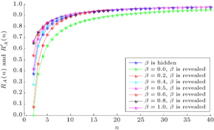
2(n 1)(n + 1)(n + 2): (11) Curve clusters of RA(n) and RA0 (n) with n and are
shown in Figures 3 and 4, respectively. They visually show the following propositions.
Proposition 6. RA(n) is monotonically increasing
functions of n and ; R0
A(n) is monotonically increasing
Figure 3. Curve clusters of RA(n) and R0A(n) as
functions of n.
Figure 4. Curve clusters of RA(n) and R0A(n) as
functions of .
Proof.
1. While 21 2; 1
, RA(n) = 1 n+11 n 12 (1 )n+1.
Obviously, RA(n) is monotonically increasing
func-tions of n and . While 20;1
2
:
RA(n) =1 n + 11 n 12 (1 )n+1
+(n + 2 2)(1 2)(n + 1)(n 1) n:
Then: dRA(n)
d =
2(n + 1)
n 1 (1 )n
2(1 2)n+2n(n+2 2)(1 2)n 1
(n + 1)(n 1)
= 2
n 1
(n + 1)(1 )n n(1 2)n 1
(1 2)n 1= 2
n 1[n((1 )n (1 2)n 1) + ((1 )n (1 2)n)
=n 12 n((1 )n (1 2)n 1)
+((1 )n (1 2)n)] ;
* 20;1 2
, ) 1 1 2 0 and (1 )2=
1 2+2 1 2 0. Hence, (1 )n (1 2)n
and (1 )n (1 2)n 1. Therefore, dRA(n)
d 0,
namely RA(n) is monotonically increasing functions
of .
Again, according to Eq. (9), let: RA(x) =
1
Z
0
x(1 t)xdt
2 4
Z
0
x
(x 1)(1 2 + t)x 1(1 t)dt
+
1
Z
x
x 1(1 t)xdt 3 7 5
=x + 1x 2 6 4
Z
0
h1(x)dt + 1
Z
h2(x)dt
3 7 5 : Then:
dh1(x)
dx =
d dx
x
(x 1)(1 2 + t)x 1(1 t)
=(1 2+t)(x 1)x 12(1 t)(x(x 1) ln(1 2+t) 1)
0 (* x 3 and 0 1 2 + t 1); dh2(x)
dx =
d dx
x
x 1(1 t)x
=(x 1)(1 t)x2(x(x 1) ln(1 t) 1) 0
)@R@xA(x)=(x+1)1 2 2 6 4
Z
0
dh1(x)
dx dt+
1
Z
dh2(x)
dx dt 3 7 5 > 0:
Hence, RA(n) or RA(x) is monotonically increasing
2. R0
A(n) = 1 2(n 1)(n+1)(n+2)(2n 1)(n+3) = 1 nn 22 1
5
2(n 1)(n+2). Obviously, R0A(n) is monotonically
increasing functions of n, owing to n 3. Eqs. (10) and (11) show complicated inuences of and n on the expected revenue. Here, both Proposition 6 and Figure 4 imply that if n is given, then there must exist 0 to satisfy RA(n) R0A(n) while
0, and RA(n) R0A(n) while 0. However,
it is dicult to x the exact value of 0with n. Next,
Proposition 7 provides some sucient conditions with respect to comparisons of both RA(n) and R0A(n).
Proposition 7. Let n 3.
1. RA(n) R0A(n) while 1
3n+1 2n(n+2)
1 n+1
;
2. RA(n) > R0A(n) while 1
3n+1 4(n+1)(n+2)
1 n+1
. Proof.
1. While 1 3n+1 2n(n+2)
1 n+1
, (1 )n+1 3n+1 2n(n+2).
* (1 )2 1 2, ) (n+2 2)
(n+1)(n 1) (1 2)n (n+2)
(n+1)(n 1)(1 )n+1. Hence:
1 n + 11 n 12 (1 )n+1
+(n + 2 2)(1 2)n (n + 1)(n 1)
1 2(n 1)(n + 1)(n + 2)(2n 1)(n + 3)
0: (12) Inequation (12) means RA(n) R0A(n) for 2
0;1
2
and, also, means RA(n) R0A(n) for 2
1
2; 1
.
Hence, according to Proposition 6, RA(n)
R0
A(n) for 2 [0; 1].
2. While 1 3n+1
4(n+1)(n+2)
1 n+1
, (1 )n+1 3n+1
4(n+1)(n+2). Then:
1 1
n + 1 2
n 1(1 )n+1
1 (2n 1)(n + 3) 2(n 1)(n + 1)(n + 2)
0: (13)
Inequation (13) means RA(n) R0A(n) for 2
1
2; 1
. * (n+2 2)(1 2)(n+1)(n 1) n 0, )
Inequation (13) also means RA(n) RA0 (n) for
20;1 2
.
Hence, according to Proposition 6, RA(n)
R0
A(n) for 2 [0; 1].
Here, RA(n) R0A(n) (RA(n) > R0A(n)) means
that expected revenue for A while revealing is less (more) than that while hiding . Proposition 7 implies that revealing the latter items in advance would uncertainly aect the overall eciency and revenues of sequential auctions, which is consistent with ndings of Cason [5], Jane and David [13], Mikusheva [9], Jackson and Kremer [10], Kannan [11], Rao et al. [16,17], and Colucci et al. [18]. Owing to RB(n) = R0B(n),
Proposition 7 is also sucient to compare R(n) with R0(n).
5. Conclusions
Focusing on sequential auctions of close substitutes with slightly more general associated valuations, this paper constructed a class Hotelling model and dis-cussed equilibrium bids under second-price sealed-bid auction formats. Conclusions showed that sequential auctions described by this model were ecient while bidders' valuations satised conditions given by Corol-lary 2. Thus, the class Hotelling model could be used as a support to deal with some auctions in supply chains. It is helpful for the analysis and design of some business mechanisms.
Through the instrumentality of this model, some sequential auctions were specically explored, while a bidder's valuation was a linear function of a distance between him or her and an item. The equilibrium bid of a bidder as a preponderant rival was deduced and veried. In addition, it depends on both numbers of bidders and locations of items whether the latter item (namely Item B) should be revealed or hidden. Gen-erally, revealing information usually improves revenues of auctions with assumptions of independent valuations for multi-items. However, our conclusions are more complicated because each bidder's valuations for Items A and B are not independent in our paper, yet are correlated. In this paper, although the sequential auctions with only two items seem simple or far-fetched, the characterization of the class Hotelling model for two items is an important step in achieving similar characterizations of models with more than two items.
Acknowledgements
We would like to thank anonymous referees for use-ful comments. This work is supported by the Na-tional Natural Science Foundation of China (Nos. 71471069, 71671135), the 2018 Soft Science Research Project of Technology Innovation in Hubei province (No. 2018ADC044), the Humanities and Social Science Research Project of Hubei Province Department of
Ed-ucation(No. 17Q068), and the Fundamental Research Funds for the Central Universities (WUT: 2019IB013). We thank them for their various contributions to this work, too.
References
1. Osborne, M.J. and Pitchik, C. \Equilibrium in Hotelling's model of spatial competition", Economet-rica, 55(4), pp. 911-922 (1987).
2. Takatoshi, T. \Multiproduct rms in Hotelling's spa-tial competition", Journal of Economics & Manage-ment Strategy, 21(2), pp. 445-467 (2012).
3. Peter, F. \Auctions with interdependent valuations", International Journal of Game Theory, 25, pp. 51-64 (1996).
4. Milgrom, P. and Weber, R. \A theory of auctions and competitive bidding", Econometrica, 50(5), pp. 1089-1122 (1982).
5. Cason, T.N. \An experimental study of information revelation policies in sequential auctions", Manage-ment Science, 57(4), pp. 667-688 (2011).
6. Beno^t, J.P. and Dubra, J. \Information revelation in auctions", Games and Economics Behavior, 57(2), pp. 181-205 (2006).
7. Silva, D., Dunne, T., Kankanamge, A., and Kos-mopoulou, G. \The impact of public Iinformation on bidding in highway procurement auctions", European Economic Review, 52(1), pp. 150-181 (2008).
8. Szech, N. \Optimal disclosure of costly information packages in auctions", Journal of Mathematical Eco-nomics, 47(4-5), pp. 462-469 (2011).
9. Mikusheva, A. and Sonin, K., Information revelation and eciency in auctions, CEPR Discussion Paper (2002).
10. Jackson, M. and Kremer, I. \The relationship between the allocation of goods and a seller's revenue", Journal of Mathematical Economics, 40, pp. 371-392 (2004).
11. Kannan, K.N. \Eects of information revelation poli-cies under cost uncertainty", Information Systems Research, 23(1), pp. 75-92 (2013).
12. Mezzetti, C. and Tsetlin, I. \On the lowest-winning-bid and the highest-Losing-Bid auctions", Journal of Mathematical Economics, 44, pp. 1040-1048 (2008).
13. Black, J. and Meza, D.D. \Systematic price dierences between successive auctions are no anomaly", Journal of Economics & Management Strategy, 1(4), pp. 607-628 (1992).
14. Zeithammer, R., Sequential Auctions with Information about Future Goods, Research Paper (2010).
15. Thomas, C.J. \Information revelation and buyer prof-its in repeated procurement competition", The Journal of Industrial Economics, 58(1), pp. 79-105 (2010).
16. Rao, C.J., Xiao, X.P., Goh, M., Zheng, J.J., and Wen, J.H. \Compound mechanism design of supplier selection based on multi-attribute auction and risk management of supply chain", Computers & Industrial Engineering, 105, pp. 63-75 (2017).
17. Rao, C.J., Goh, M., Zhao, Y., and Zheng, J.J. \Location selection of sustainability city logistics cen-ters", Transportation Research Part D: Transport and Environment, 36, pp. 29-44 (2015).
18. Colucci, D., Doni, N., and Valori, V. \Preferential treatment in procurement auctions through informa-tion revelainforma-tion", Economics Letters, 117(3), pp. 883-886 (2012).
Biographies
Erqin Hu received an MS degree from Huazhong University of Science and Technology, China in 2005 and received her PhD degree from Huazhong University of Science and Technology, China in 2017. Her research interests include auction theory and decision theory and method.
Congjun Rao received an MS degree from Wuhan University of Technology, China in 2006 and received his PhD degree from Huazhong University of Science and Technology, China in 2011. His research interests include supply chain management, auction theory, and decision theory and method.
Yong Zhao is currently a Professor at the Department of Control Science and Engineering of Huazhong Uni-versity of Science and Technology. His BSc, MSc, and PhD degree were obtained from Huazhong University of Science and Technology in Systems Engineering. His main research interests include decision theory and methods, engineering economics, and auction theory.