1181.pdf

KUO-HSI CHENG. The Influence of Environmental Tobacco Smoke on

the Lifetime Probability of Lung Cancer due to Exposure to Radon

ABSTRACT

An analysis concerning the effect of environmental tobacco

smoke (ETS) on estimation of lifetime risk of radon-induced lung

cancer is made. Based on the consideration of radon dosimetry as a

function of age, a generalized state-vector model is used to estimate

the total probability of lung cancer due to exposure to both radon

and ETS during a normal (73 year) lifespan. This report suggests

that there is a general tendency of increasing working level

concentration of radon progeny and decreasing unattached fraction

of radon progeny RaA (Po-218) with greater amounts of ETS present

in the home. The initial concentration of ambient aerosols plays an

important role in quantifying the effect of ETS on radon exposure.

The combined ETS and radon exposure may either raise or lower the

risk of lung cancer associated with radon exposure alone, primarily

depending upon the initial aerosol concentration and amounts of

cigarette smoke.

ACKNOWLEDGEMENT

I would like to extend appreciation to my research advisor, Dr. D. J. Crawford-Brown, for his encouragement, support, guidance throughout the development and completion of this study and during

my graduate training. The other members of the advisory committee. Dr. A. G. Turner and Dr. J. E. Watson, are gratefully acknowledged for their review and valuable suggestions in preparation of this report.

I am indebted to Dr. W. Hofmann who generously provided his computer code for calculating the dose of radon progeny. In addition, gratitude is also expressed to my girlfriend, Yi-Hsin Yang, who assisted in computer work of fitting the spline functions and provided the moral and emotional support during the hard time of

preparing this report.

This report is especially dedicated to my parents and family in

Taiwan.

TABLE OF CONTENTS

Page

LIST OF TABLES ... vi

LIST OF HGURES... viii LIST OF ABBREVIATIONS ... ix

Chapter

I. INTRODUCTION ... 1 1.1. A Brief Review of Radon... 2 1.2. A Brief Review of Environmental Tobacco Smoke .... 4

n. THEORETICAL FRAMEWORK... 6

2.1. Estimation of Exposure Conditions ... 6

2.2. Calculation of Deposition and Doses ... 1 2

2.3. Risk Estimation... 1 3

2.3.1. Description of State-Vector Model ... 14

2.3.2. Mathematical Formulations ... 1 8

2.3.3. Equation Solutions... 2 0

III. DETERMINATION OF PARAMETER VALUES... 2 5

3.1. Parameters in Estimation of Exposure Conditions ...2 5

3.2. Parameters in State-Vector Model ... 2 6

3.2.1. Rate Constants for Background Transition ... 2 8

a. Spontaneous Rate of Mitosis (Ms)...2 8

State 0 to State 1 (kos)... 3 5

State 1 to State2 (kis)... 3 7

State 3 to State 4 (kss)... 3 8

e. Spontaneous Rate of Transition from

State 4 to State 5 (k4s)... 3 8

3.2.2. Radiation Induced Rates...3 8

IV. RESULTS...4 1

V. DISCUSSION... 4 8

VI. RECOMMENDATIONS FOR FUTURE RESEARCH... 5 1

REFERENCES... 5 4

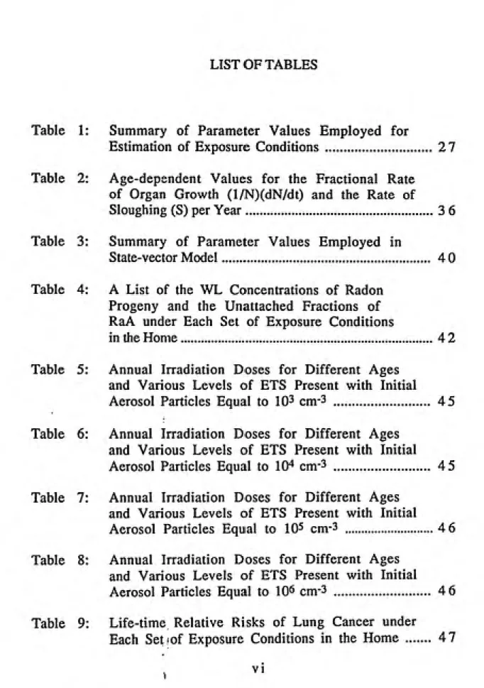
LIST OF TABLES

Table 1: Summary of Parameter Values Employed for

Estimation of Exposure Conditions ... 27

Table 2: Age-dependent Values for the Fractional Rate

of Organ Growth (l/N)(dN/dt) and the Rate of

Sloughing (S) per Year...3 6

Table 3: Summary of Parameter Values Employed in

State-vector Model... 4 0

Table 4: A List of the WL Concentrations of Radon

Progeny and the Unattached Fractions of

RaA under Each Set of Exposure Conditions

in the Home...4 2

Table 5: Annual Irradiation Doses for Different Ages

and Various Levels of ETS Present with Initial

Aerosol Particles Equal to 10^ cm-3 ... 4 5

Table 6: Annual Irradiation Doses for Different Ages

Aerosol Particles Equal to lO^ cm-3 ... 4 5

Table 7: Annual Irradiation Doses for Different Ages

and Various Levels of ETS Present with Initial

Aerosol Particles Equal to 10^ cm-3 ...4 6

Table 8: Annual Irradiation Doses for Different Ages

Aerosol Particles Equal to 10^ cm-3 ... 4 6

Table 9: Life-time Relative Risks of Lung Cancer under

Each Set of Exposure Conditions in the Home ... 47

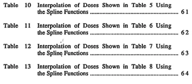
Table 10 Interpolation of Doses Shown in Table 5 Using

the Spline Functions... 6 1

Table 11 Interpolation of Doses Shown in Table 6 Using

the Spline Functions... 6 2

Table 12 Interpolation of Doses Shown in Table 7 Using

the Spline Functions... 6 3

Table 13 Interpolation of Doses Shown in Table 8 Using

the Spline Functions... 6 4

LIST OF FIGURES

Figure 1: Flow Diagram for Various Fates of Radon Progeny

Figure 2: State-vector Model... 15

Figure 3: Model for Background Transition ...2 9

Figure 4: Model for Spontaneous Mitosis... 3 0

Figure 5: Age Dependence for Fractional Rate of Change

of the Organ Masses (yr') for the Human ... 3 3

Figure 6: Partial Summary of the Data Used to Develop a

Relationship Between the Mass and the Biological

Half-time in the Whole Body...3 4

Figure 7: Age Dependence of Organ Masses for the

Human... 3 4

LIST OF ABBREVIATIONS

BEIR Committee on the Biological Effects of Ionizing Radiations

EPA Environmental Protection Agency

ETS Environmental Tobacco Smoke

MMAD Mass Median Aerodynamic Diameter

MS Mainstream

NCRP National Council on Radiation Protection and

Measurements

NOPL Naso-oro-pharyngo-laryngeal

NRC National Research Council

RaA Progeny Radium A (Po-218)

RaB Progeny Radium B (Pb-214)

RaC Progeny Radium C (Bi-214)

RSP Respirable Suspended Particulates

SS Sidestream

TB Tracheobronchial

WL Working Level

WLM Working Level Month

1. INTRODUCTION

The health risks related to indoor radon and environmental

tobacco smoke (ETS) are of great public concern. The evidence from

epidemiological studies of uranium miners and from animal

experiments suggests that there is a strong association between

exposure to radon and lung cancer (NRC88). However, the

relationship between ETS and lung cancer is controversial at the

moment. Some studies have concluded that exposure to ETS causes

lung cancer, but others found no significant effect. It is noted that

many previous studies have been conducted to assess each of these

two pollutants associated with lung cancer separately, but little

attempt has been made to examine the combined risk from exposure

to radon and ETS simultaneously.

The purpose of this study is to estimate the lifetime risk of

radon-induced lung cancer by considering the effect of ETS on the

tracheobronchial (TB) distribution and dose of radon progeny. In

addition, the issue of radon dosimetry as a function of age will be

taken into account in calculating the delivered dose to the lung for

each age.

Chapter 2 explains the theoretical framework for estimating

the lifetime risk of lung cancer attributable to exposure to radon and

ETS. This includes the assumptions, mathematical models, and

solutions for estimating exposure conditions, deposition of radon

progeny, doses to the lung, and the probability of developing lung

cancer.

Chapter 3 discusses the parameter values used in estimating

exposure conditions; and, the parameter values used in the

state-vector model for estimating the lifetime risk of lung cancer.

Chapter 4 presents the final results, including the effect of ETS

on radon progeny working level (WL) concentration and unattached

fraction of progeny RaA; the annual doses under each set of exposure

conditions for each age; and, the different ratios of risks (with

ETS/smoke free) under each set of exposure conditions.

Chapter 5 discusses the implications of the results found in this

study, including the relevance to other studies and interpretation for

mitigation purposes.

Chapter 6 includes further investigations and recommendations

for future research.

1.1. A Brief Review of Radon

Radon is a radioactive gas occurring naturally by alpha decay

of radium-226 in rocks and soil. As radon undergoes the radioactive

decays , it decomposes into short-lived decay products called radon

progeny. Radon progeny are chemically active and believed to

contribute a major portion of the biologically significant doses when

they deposit in the lung. Indoor airborne radon arises principally

from the following sources : the basement floor under which the

rocks and soil are located, many building materials, and

containing water supply. Since radium can be found almost

everywhere in the earth's crust, all homes actually contain some

levels of radon. Due to the ubiquity of radon in homes, there is a

growing concern about its associated health risks among the general

population. ;

In the 1988-1989 home surveys in 25 states conducted by the

U.S. Environmental Protection Agency (EPA87), homes in many states

have a radon concentration exceeding the action level (4 pCi/L) set

by the EPA. Among these surveyed states, Iowa (71%), North Dakota

(63%), and Minnesota (46%) have the highest percentage. Even

though indoor radon concentration varies from home to home, which

is basically dependent on house characteristics and geological areas,

an annual average radon level of 0.83 pCi/L or 0.004 working level

(WL) is used by the EPA for estimating the health risk associated

with radon exposure (EPA 87).

There have been a number of investigations of radon-related

health risks of underground miners since the United Nations

Scientific Committee on the Effects of Atomic Radiation (UNSCEAR)

1977 report was issued (NRC90). Because different models and risk

coefficients were used, the risk estimates due to radon exposure vary

significantly, ranging from 130 to 730 deaths out of 10^ persons per

working level month (WLM). For example, the Biological Effects of

Ionizing Radiations (BEIR) III Committee used a constant absolute

risk model which generated the highest estimate of 730 deaths per

10^ person WLM. The National Council on Radiation Protection and

Measurement (NCRP) used an absolute risk model with exponentially

decreasing risks with time after exposure and projected a lowest

estimate of 130 deaths per 10^ person WLM. In contrast, the BEIR

IV committee used the time and age dependent relative risk model

which resulted in a moderate estimate of 350 attributable lung

cancer deaths per 10^ person WLM. Overall, the lifetime risk of lung

cancer due to indoor radon exposure is about 400 per million persons

per WLM, and the lifetime exposure dose is approximately 15 WLM

(Lao90).

The EPA estimated a radon-exposed lung cancer mortality rate

of 5,230 to 20,894 per year in the United States. This implies that a

probability of 23 to 92 excess lung cancer deaths for each one million

people per year is attributable to indoor radon exposure (Lao90).

1.2. A Brief Review of Environmental Tobacco Smoke

ETS is a complex substance containing over 4,000 chemicals, which

primarily comes from a combination of sidestream (SS) smoke

released from the burning end of the cigarettes and exhaled

mainstream (MS) smoke emitted from the smokers. The SS smoke

contributes the major constituents to ETS. Each mixture, SS, MS, and

ETS, is an aerosol consisting of a particulate phase and a vapor phase.

The concentration of many carcinogenic and other toxic compounds

is higher in SS smoke than in MS smoke. Included are ammonia,

volatile amines, volatile nitrosamines, nicotine decomposition

products, and aromatic amines (NRC86). Many field studies and

mathematical models have demonstrated that ETS is one of the major

potential sources of indoor air pollutants and contributes a significant

portion of particles to indoor air pollution.

The potentially adverse effects of ETS may range from

irritation or acute respiratory disease to fatal lung cancer due to

regular long-term exposure. Since mainstream smoke is believed to

cause lung cancer, the possibly qualitative similarities between ETS

and mainstream smoke make it reasonable to suspect that long-term

exposure to ETS might increase the risk of developing lung cancer.

The National Research Council (NRC) concluded that

epidemiological studies have demonstrated an association between

lung cancer in non smokers and ETS exposure, and that laboratory

experiments provide a biological plausibility for ETS to cause lung

cancer in human cells (NRC86). Based on the review and analysis of

24 epidemiological studies, a formal risk assessment done by EPA

concluded that ETS is a Group A carcinogen known to cause lung

cancer in human (EPA90). However, a number of scientists have

suggested that epidemiological studies of ETS are not reliable due to

the possibility of recall bias, misclassification, and other

methodological problems. The risk assessment of ETS based on these

questionable studies can not prove the causality between ETS

exposure and increased risk of lung cancer. The difficulty in

identifying ETS effects arises primarily for the following three

reasons : (1) ETS is a complex mixture containing over 4,000

components whose biological effects can not be precisely quantified

given the relatively insensitive techniques available, (2)

epidemiology is too blunt a tool to distinguish between "very low

risk" and "no risk" of lung cancer from ETS (Roe90), and (3) ETS may

interact with numerous other indoor air pollutants, including radon,

asbestos, formaldehyde, and others.

11. THEORETICAL FRAMEWORK

To predict the lifetime risk of lung cancer attributable to

exposure to radon and ETS, the risk assessment is broken into the

following analytical steps : (1) estimation of the exposure conditions

for radon with and without ETS present, (2) calculation of the

deposition of radon progeny in the tracheobronchial (TB) region of

the lung under each set of exposure conditions, (3) calculation of the

doses to the epithelial cells in each generation of the lung under each

set of exposure conditions, and (4) calculation of the probability of

lung cancer from these doses under each set of exposure conditions.

2.1. Estimation of Exposure Conditions:

In this study, the radon concentration in indoor air is assumed

to remain at a constant value of 1 pCi/L, which is reported as the

approximate average indoor concentration of radon in the U.S.

(NCRP84). The indoor progeny derive from the radioactive decay of

airborne radon in the home and transport through ventilation from

the outside atmosphere. A fraction of the radon progeny exists in a

free form called the unattached fraction, while the remainder is

attached to aerosol particles. Free progeny with a positive charge

will undergo one of the following fates:

(1) They migrate onto room surfaces to which they are

attached.

(2) They attach to aerosol particles in the room, and are

either inhaled along with the particles, deposited on room

surfaces along with the particles, or released from

particles into a free form again due to recoil during

subsequent decay.

(3) They remain free in air and eventually will be inhaled.

A block diagram depicting the general features of the decay,

transport, and attachment of radon progeny is shown in Figure 1.

Several parameters appearing in Figure 1 are defined as

follows: (1) Xi (time-i) is the radioactive decay rate constant for the

ith progeny, (2) Xy (time-i) is the rate of ventilation, (3) X^j and X.d,a

(time-i) are the rates of deposition onto room surfaces for free and

attached progeny, respectively, (4) ai is the fraction of the i^h

attached progeny that release from attachment to aerosol particles

during subsequent decay, and, finally, (5) Xs (time-i) is the rate of

attachment of free progeny to aerosol particles.

The relation between X^ and ambient particle conditions is

given in the form of (NRC88):

?is =Njtd2 v/4 (1)

Where: N= concentration of particles in air (cm-3)

d = median diameter of particles in air (cm)

V = mean ion velocity in air (cm/sec), employed here

r_{Concentration 1} Concentration 1

of free of attached

progeny i-1 in the home

progeny i-1 in the home

Ci-i.f 1

Ci-i,a 1

Xi-i

/

\!/ _K \l/

1 Concentration!

1 r\f fr^^ L

Av

>

1 Concentration

[Xs

of attached

progeny i in the home

Ci,a

Xv Concentration 1

of attached progeny i outdoors Ci,o / ---7 progeny i

outdoors 1

1 Ci.o.f f

/

progeny i

J in the home

1 Ci,f

\y

Xv Xv

Xd,f y^ M

/Xioti

\/

f

\

Room surfaces Concentration

of free

Concentration

of attached

Room surfaces

in the home

progeny i+1

in the home

Ci+i,r

progeny i+1 in the home

Ci+i,a

in the home

Figure 1 Flow Diagram for Various Fates of Radon Progeny

in the Home

From the flow diagram shown in Figure 1, two differential

equations in the form of general expressions for the i^h progeny may

be written to describe the rate of change of concentrations of the

progeny which are either free (Ci,f(t)) in air or attached to aerosol

particles (Ci,a(t)) :

d Ci,f(t)

= ?lilCi.i,f(t) + XvCi,o,f(t) + ?.iiaiiCi.i,a(t) Xd,fCi,f(t)

-d t ?ivCi,f(t) - XiCi,f(t) - ?isCi,f(t) (2)

d Ci,a(t)

--- = ?^vCi,o,a(t) + >-sCi,f(t) + Xi.i(l - ai.i)Ci.i,a(t) - >.d,aCi,a(t)

d t ?iiaiCi,a(t) - ?ivCi,a(t) - Xi(l-ai)Ci,a(t) (3)

Here, the subscript i equal to A represents the progeny RaA

(Po-218), i equal to B represents the progeny RaB (Pb-214), and i

equal to C represents the progeny RaC (Bi-214); the subscript f

denotes the free progeny (unattached to aerosol); the subscript o

means the outdoor atmosphere; and, the subscript a stands for the

progeny attached to aerosol particles.

In an undisturbed area with little air circulation, the short¬

lived progeny will come into equilibrium with the parent radon

(NCRP85). Upon reaching the state of equilibrium, the progeny

concentrations will not change with time. This means that equations

(2) and (3) may be solved at equilibrium by setting dCi,f(t)/dt and

of indoor radon (C222) and outdoor progeny (Ci,o,f and Ci^o.a) are

At equilibrium, the concentrations of progeny are:

^222 C222 + '^V CA,o,f CA,f

=---Xd,f + ?tv + ^A + ?^s (4)

^v C-A.o.a + ^s CA,f

Ca a =---_-A,a

Cfi.f =ͣ

>^d,a + ^A + ^v (5)

^A CaJ + ^v CB,o,f + ^A OCA CA,a

?ld,f + ^v + ^B + ^s (6)

K CB,o,a + ^s Cfi.f + X,A (1 -aA) CA,a

Cc,f=->^d,a + ^B + ^v (7)

^B CB,f + X,v Cc,o,f + ^B Wb CB,a

^d,f + ^v + ^C + ^s (8)

^v Cc,o,a + ^s Cc,f + X,B (I-wb) CB,a

Cc,a

—---Ua + >-C + ?^v (9)

In equations (4)-(9), the units of the concentrations are atoms

per liter of air (atoms/L). From the report of the NCRP (NCRP85), the

approximate number of atoms per pCi is 18,000, 10, 85, and 63 for

ͣ

Rn, RaA, RaB ,and RaC, respectively. Concentrations in pCi/L may be

obtained by dividing the results of equations (4)-(9) by the

appropriate conversion factor from the NCRP report.

Working level (WL) is the common unit employed in risk

analyses for radon progeny, originally in uranium mines but now in

environmental exposures as well. Numerically, the WL is any

combination of short-lived progeny in one liter of air that will result

in the emission of 1.3 x 10^ MeV of potential alpha energy (NCRP88).

It is calculated from the following relation (Ev68):

WL = 0.00103 (CA,f + CA,a) + 0.00507 ( CB,f + CB,a )

+ 0.00373 ( Cc,f + Cc,a) (10)

In equation (10), all concentrations are expressed in units of pCi/L.

The presence of ETS will influence the concentration of aerosol

particles to which the radon progeny may attach. The results of

measurements of the mean diameter of particles in SS smoke have

been reported in several studies. The mass median aerodynamic

diameter (MMAD) for ETS particles was measured by McCusker et al.

(Mc83) and ranged from 0.37 to 0.52 ^m, which is similar to the

results obtained by Keith (Kei60) using a specially modified

centrifuge. The aging of ETS will reduce the MMAD by a factor of 2

to 3 due to the loss of larger particles by settling (Kei60, Wy67,

In85). Therefore, the MMAD for ETS particles is approximately 0.15

[im, which is consistent with the MMAD for ambient indoor aerosols

to which radon progeny normally are attached without the presence

of ETS. This implies that the addition of ETS changes the

concentration (N) but not the diameter (d) of particles in air in

equation (1).

2.2. Calculation of Deposition and Doses

Based on the fact that the observed lung cancers among

uranium miners appear to occur primarily in the TB region (Mc80),

the basal cells of the bronchial epithelium are regarded as the most

radiosensitive and are the target cells for lung cancer induced by

radiation from radon progeny. The calculation of deposition

probability in the TB region for radon progeny is determined by the

breathing rate, the size distribution and the unattached fraction of

progeny, and the filtration efficiency of the nasopharyngeal region

(Lao90). While several processes contribute to the deposition of

aerosol particles in a cylindrical tube like the lung airway, the three

most important mechanisms of deposition are impaction,

sedimentation, and diffusion. The total probability, P(n), of a particle

depositing in the n^h generation of the lung is given by (C-B87):

P(n) = 1 - [ 1 - Pi(n) ] [ 1 - Ps(n) ] [1 - PoCn) ] (11)

where, Pi(n), Ps(n), and PoCn) represent the fractions of particles

which deposit by impaction, sedimentation, and diffusion,

respectively, in the n^h generation.

After calculating total deposition in each generation of the lung

for the radon progeny, the radiation dose is estimated by the

following steps : (1) mucus flow is modeled to calculate how the

progeny move; (2) this movement is used to estimate the site of

decay for the progeny, yielding decays/cm^ in each generation

during a year of exposure; (3) depth-dose curves are developed to

yield dose per decay/cm^; and, finally (4) dose to basal cells is

calculated by multiplying the result of (2) and (3). This dose

calculation based on the location of critical cells relative to the site of

decay for progeny takes into account the shielding effect of

mucociliary layer, mucus thickness, bronchial morphometry, and

other factors. The detailed processes for modeling movement on the

mucociliary blanket, computing areal density of the radon progeny

on the walls of the generations, and generating depth-dose curves

refer to "Dosimetry" by Crawford-Brown (C-B87).

For purposes of this report, deposition of progeny in the

generations of the TB region and dose to basal cells of the lung were

calculated using the computer code of Hofmann.

The age-variant doses under each set of exposure conditions

are shown in Tables 5 to 8.

2.3. Risk Estimation

The generalized state-vector model of radiation carcinogenesis

by Crawford-Brown and Hofmann (C-B90) has been demonstrated to

successfully explain patterns found in experimental or

epidemiological studies involving radiation and cancer. The concept

of this model is that a cell must pass through several distinctive

stages to produce a fatal tumor. Unlike the multistage model, the

state-vector model specifies the biophysical meaning of each

transition and stage in terms of initiation, promotion, and

progression.

Initiation is triggered when a cell experiences DNA damage and

has undergone a required number of divisions. The whole process of

initiation is characterized by the following four steps : (1) inception

of a first specific DNA strand break, (2) occurrence of a second less

specific DNA strand break, (3) interaction of the above two breaks,

and (4) division-related fixation of this primary damage. Promotion

is produced by the loss of contact inhibition in a focus of cells, which

for radiation occurs due to the loss of proliferative capacity in a

fraction of the cells surrounding an initiated cell (C-B90).

Progression is associated with the growth of the promoted cells into a

frank tumor. This transition is related to the kinetics of growth,

death, and removal of cancer cells.

In the following risk estimation, this model will be used to

calculate the lifetime probability of lung cancer. The lifetime risk of

lung cancer is assumed to be proportional to the number of cells

reaching the state of progression during a normal (73 year) lifespan.

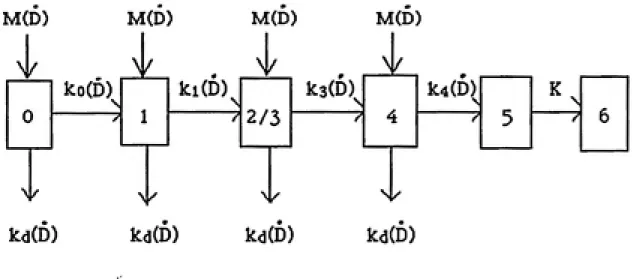
2.3.1. Description of State-Vector Model

The model is designed to describe radiation induced cellular

transformation by assuming that an initially undamaged cell must

pass through 7 states (from state 0 to state 6) to yield a colony of

transformed cells, especially for alpha irradiation due to radon

exposure. The features of the model may be found in figure 2 and

the details are discussed below.

State 0 refers to cells in a normal and undamaged state. Cells

in state 0 have not yet experienced any lesion after exposure to

radiation or chemicals starts.

M(D) M(D) M(D) M(D)

V V . V -

0

koCD)

1

kiCD)

2/3

lC3(D)^

4

k4(D) 5

K 6

/ / / >>

N^ \p N^

kd(D) kd(D) k<j(D) k<3(D)

Where: Numerical number i (i.e. from 0 to 6) represents state i

M(D) is the rate of mitosis (day-l)

kd(D) is the rate of cell killing (day-i)

ki(D) is the rate of transition for state i (day-1)

K is the fraction of cells in state 5 moved to state 6

State 1 is reached when a cell has experienced a specific DNA

strand break. The transition from states 0 to 1 is assumed to be

m

characterized by first-order kinetics with a rate constant ko(D),

which is a function of the dose rate D during each year of exposure.

It is important to bear in mind here and in the remaining discussion

that D will vary with age due to changes in breathing characteristics

and lung anatomy.

A cell reaches state 2 when it suffers a second less specific DNA

double strand break(C-B90). This transition governed by first-order

* •

kinetics with a rate constant ki(D) is also a function of dose rate D.

State 3 represents an interaction between the first and the

second DNA double-stranded breaks, which for alpha irradiation

occurs immediately after a cell has reached state 2.

The transition to state 4 is the result of cell division. During

each division, only a required fraction (P4) of cells in state 3 are

moved into state 4 (C-B90). This transition is referred to as

division-related fixation of primary lesions, with a rate constant k3(D) which

is dependent on the rate of mitosis of cells in state 3. This rate of

mitosis is related to D due to stimulation of cell division by

cytotoxicity.

The transition of a cell to state 5 is the result of promotion. As

m

discussed earlier, the rate of promotion k4(D) contains a spontaneous

rate and a radiation induced component. This radiation-induced

transition occurs when a required fraction of the cells surrounding a

state 4 cell loses proliferative capacity. From histological

considerations, an epithelial cell is found to be surrounded by six

four out of these six neighboring cells are killed (C-B90). The loss of

proliferative ability of dead cells interrupts cellular inter¬

communication within the community to yield an uncontrolled

growth of cells in state 5. This is referred to as contact inhibition

A cell in state 6, the final state, has progressed from a

preneoplastic lesion to a frank tumor. The study of atomic bomb

survivors suggests that the latency period of cancer is not

significantly affected by radiation (Shi90). Based on this information,

it is assumed here that a fraction K of state 5 cells are moved to state

6, and that K is not a function of D. This implies that any cell

reaching state 5 has an equal chance to produce cancer regardless of

time or dose rate.

Prior to state 5, there are rate constants for cell killing, Kd(D),

and for the mitosis of cells, M(D), in each state, respectively. These

two transition rates are assumed to include a spontaneous rate,

which is based on the belief that a natural transition would occur

without any delivered dose, and a radiation induced rate, which is

considered to be governed by linear kinetics (details discussed in the

next chapter). In addition, the spontaneous rate of mitosis is an

age-dependent parameter due to organ growth prior to adulthood. Both

spontaneous rates, therefore, change with age.

To complete the final risk estimation, the interaction of ETS and

radon progeny must be taken into account. A multiplicative model is

used to depict the mechanism of interaction (NRC88). This model

assumes that ETS acts as a promoter in the process of carcinogenesis

RR = RRradon ( 1 + 0.024 n ) (12)

where RR is the final estimate of relative risk of lung cancer, RRradon

is the relative risk from radiation alone, and n is the rate of

cigarettes smoked (in units of packs per day). Given a recent report

from experimental data (Gri88), the particulate phase of cigarette

smoke is considered to contain the primary carcinogens for most

induced cancers. It is assumed that the mass of respirable

suspended particulates (RSP) deposited in the TB region is an

appropriate measurement of carcinogenicity for both MS smoke and

ETS. Therefore, the conversion from exposure to MS smoke to

exposure to ETS is based on the assumption that the total deposition

of RSP in the TB airways is an approximate measure of equivalence

(NRC86). The total inhaled mass of RSP has been calculated by Wells

(WeSS) to be 240 mg for the active smoker and 3 mg for the passive

smoker. Multiplying these values by the TB deposition fractions

(C-B82) yields 36 mg of total deposited RSP for the active smoker and

0.12 mg of total deposited RSP for the passive smoker. If an active

smoker consumes one pack of cigarettes per day in the home, the

passive smoker would inhale a mass of RSP equivalent to 0.08

cigarettes per day. Multiplying this quantity by the excess risk of

smoking miners (i.e. 0.3) yields a value of 0.024. This implies that

there is an increased risk of 2.4% in the presence of ETS equal to one

pack of cigarettes per day when the promoting effect of ETS is

considered in the radon-induced carcinogenesis.

2.3.2. Mathematical Formulations

The quantitative characterization of state-vector model is

simply based on the concept that the rate of change of each state is

equal to total rate in minus total rate out. Let Ni(t) be the number of

cells of the lung in state i at time t after exposure to radon starts. In

Figure 2, each box prior to state 5 has a mitotic rate constant M(D)

feeding in and a rate constant of cell killing kd(D) flowing out. The

product of Ni(t) and M(D) means the rate of cell increase derived

from cell division, while the value of Ni(t) times kd(t) represents the

rate of cell loss due to cell killing. Because of the prompt interaction

between states 2 and 3 for alpha irradiation, this should not be

considered as a distinctive transition. A single box representing both

state 2 and state 3 is used in the state-vector model for the present

study.

Based on the above discussion, the differential equations

dN^(t)

dt

dN^(t)

dt

dN3(t)

dt

= M(D) N^Ct) - ( k^(D) + k^CD) ) N^Ct) (13)

k^(D) N^(t) + ( M(D) - k^(D) - k/D) ) Nj(t) (14)

kj(D) N/t) + ( M(D) - k3(D) - k^(D) ) N3(t) (15)

dN^Ct)

dt

= kgCD) N3(t) + ( M(D) - k3(D) - k^(D) ) N^Ct) (16)

State 5 is given separately by integral equation due to the

constant K independent of dose rate. This means that cells reaching

state 5 will pile up and undergo the transition to state 6 with a fixed

fraction K.

T

N3(t)= Jk^CD) N/t) dt (17)

0

But, Ng(t) = K N5(t) (18)

T

Ng(t)= K jk/D) N^(t) dt (19)

0

Therefore, the total probability of lung cancer is:

P^(D,t)= JKk^(D) N^(t) dt (20)

0

2.3.3. Equation Solutions

Through repetitive applications of Bernoulli's solution (Kel60),

the above differential equations are solved as follows:

No(t) = No(0) e - ('^d(D) + MD) - M(D) ) t ^^l)

ko(D)No(0)

Nj(t)= ---(e'^' -e"^' ) + N,(0)e"^' (22)

B -A

k,(D)kJD)NJO) e"^'-e"^' e"^'-e'^'

B - A C - A C-B

NjCt) =---

ͣ

---(---)

ki(D)N^(0)

C-B

+---(e'^'- e'^') + NgCO) e"^' (23)

kgCD) kj(D) k^(D) Nq(o) e'^' - e'^' e"^' - e"°'

N^d)

=---(---(B-A)(C-A) D-A D-C

k3(D) k^(D) k^CD) Nq(0) e'^' - e"°' e'^' - e"^'

(

(B-A)(C-B) D-B DC

o #

k3(D) kj(D) Nj(0) e"^'- e'^' e'^' - e"^'

_---(---C-B D-B DC

k3(D)N3(0)

DC

+---(e"^' - e"^') + N,(o) e"^' (24)

k^(b) kgCD) kj(D) kp(D) Np(0) 1 e'^' -1 e""^'-1

N5(t)=--- [--- (---)

(B-A)(C-A) D-A D A

1 e"^^ -1 e"^^ -1

DC D

k^ii)) k^(D) kj(D) k^iD) Nq(0) 1 e"^' -1 e"^' -i

---[---(---)

(B-A)(C-B) D-B D B

1 e'^^ -1 e-^^ -1

(---)]

D-C D

• •

k^ij)) k3(D) kj(D) N^(0) 1 e'^' -1 e'^' -1

+---[---(---C-B D-B D B

1 e-^^-1 e-'^^-i

)]

DC D

k^(D) k3(D) N3(0) e"^' -1 e'^' -1

(

DC D C

k^CD) N^CO)

( e'^'- 1 ) + N,(0) (25)

D

Where:

A = k^(D) + k^CD) - M(D)

B = k^(D) + k^(D) - M(D)

C = k^(D) + k3(D) - M(D)

D = k/D) + k^CD) - M(D)

As discussed earlier, it is assumed that the lifetime probability of lung cancer is proportional to the number of cells reaching the

state of progression (i.e. state 6) during a normal 73-year exposure. Meanwhile, any cell reaching state 5 will undergo the transition to

state 6 with a constant fraction regardless of age. Based on the assumption of a 20-year latency period for developing lung cancer, the number of cells reaching state 5 after a 53-year exposure (i.e. N5(53)) can be a measuring scale proportional to the lifetime risk of

lung cancer. |

To calculate the accumulative probability of lung cancer, the method of dividing the lifetime into intervals assumes a constant

annual dose during each year. This means that those

dose-dependent parameter values appearing in equations (21) to (25) are

constant within a given year. The annual doses are interpolated

using the spline functions to fit a smooth curve among the given data

shown in Tables 5 to 8. The detailed discussion refers to Appendix.

The initial condition for calculating the number of cells

reaching each state at age 1 is obtained by arbitrarily setting one cell

in state 0 at age 0. Inserting No(0) = 1, Ni(0) = NsCO) = N4(0) = NsCO)

= 0, and the corresponding parameter values into equations (21) to

(25) yields the number of cells in each state at age 1. This obtained

vector at age 1 in turn provides the initial condition for calculating

the number of cells reaching each state at age 2. Repeating the same

computing process, the number of cells reaching state 5 at age 53 can

be calculated under each set of exposure conditions using computer

dividing the number of cells in state 5 with different amounts of ETS

present by that with smoke free for differing initial aerosol

III. DETERMINATION OF PARAMETER VALUES

3.1. Parameters in Estimation of Exposure Conditions

The values of various parameters appearing in equations 4 to 9

must to be determined to estimate the exposure conditions.

Assuming a rate of one entire air circulation per hour for

typical home conditions, a value of 0.0167 min-1 for the ventilation

rate is assumed here. The decay rate constants for Rn, RaA, RaB, and

RaC are 1.26 x 10-4, 0.227, 0.026, and 0.035 min-i(NCRP8 8),

respectively. The value of 0.2 min-^ for X,d,f is the average of values

determined by Rudnick and Maher (Ru86) and the NCRP (NCRP84),

while the value of 0.0167 min-i for Xd.a is adopted from the NCRP

(NCRP84) and is applicable to the deposition of cigarette smoke. The

fraction of decay for attached RaA that results in unattached RaB, aA,

is approximately equal to 1/2, but for attached RaB (as) or attached

RaC (ac) is zero (Raa69). Since the MMAD for both natural aerosols

and tobacco smoke particles is approximately identical, the value of

0.15 ^m for d is used in equation (1).

In solving for Xs, the aerosol density (N), which is affected by

the presence of tobacco smoke must be specified. From the report of

the NRC (NRC86), a consumption of 1 pack of cigarettes per day will

produce 26 mg of RSP per hour. For a typical home volume of 400

m3 with ventilation rate equal to 1 hr-i, this rate of release will add

an increased aerosol content of 60 [ig/m^. This amount is equivalent

to an increased aerosol density of approximately 2 x 10^ cm-3 and

must be added to the initial particle concentration without ETS

2 packs of cigarettes per day. Therefore, an increased amount equal

concentration for 1/2 and 2 packs of cigarettes per day, respectively.

Tablel provides a detailed list of the values of various

3.2. Parameters in State-Vector Model

The values of parameters employed in the state-vector model

are assumed to contain a spontaneous rate and a radiation-induced

component. This yields the following mathematical formulations:

M(D) = Ms-I-Mr(D) (26) kd(D) = kds + kdRD (27) ko(D) = kos + koR D (28)

ki(D) = kis + kiRD (29)

k4(D) = k4s + k4R(D) (31)

Here, subscript s refers to the spontaneous component and

subscript R denotes the radiation-induced component in each of the

above equations.

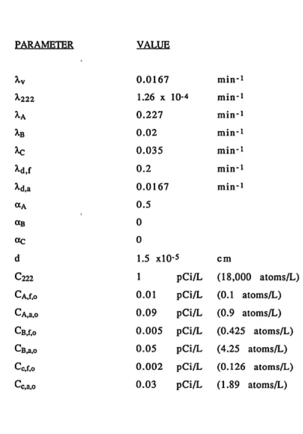
Table 1 Summary of Parameter Values Employed for

Estimation of Exposure Conditions

PARAMEIER VALUE

^^ 0.0167 min-i

^222 1.26 X 10-4 min-i

^A 0.227 min-i

^B 0.02 min-i

Xc 0.035 min-i

^d,f 0.2 min-i

^d,a 0.0167 min-i

"A 0.5

ttB 0

oc 0

d 1.5 xlO-5 cm

C222 1 _{pCi/L (18,000 atoms/L)}

Caj.o 0.01 _{pCi/L (0.1 atoms/L)}

CA,a,o 0.09 _{pCi/L (0.9 atoms/L)}

CB,f,o 0.005 _{pCi/L (0.425 atoms/L)}

CB,a,o 0.05 _{pCi/L (4.25 atoms/L)}

Cc.f.o 0.002 _{pCi/L (0.126 atoms/L)}

Cc,a,o 0.03 _{pCi/L (1.89 atoms/L)}

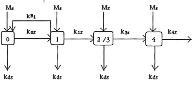
3.2.1. Background Transition Rates:

In the case of a natural transition, cell repair from state 1 back

to state 0 occurs. This background rate of repair, 0.13 hr^, is

independent of dose rate (discussed later) and taken from in-vitro

studies (Roo90). The block diagram for background transition prior

to state 4 is depicted in figure 3.

The rate constants for background transition (kos, kis, k3s) are

determined by the equilibrium values of No(t), Ni(t), and N3(t)

without exposure to radon progeny at t equal to 0. These

equilibrium values (Nqe, Nie, and Nse) calculated by Crawford-Brown

and Hofmann using in-vitro data are equal to 0.94, 0.06, 0.001,

respectively (C-B90).

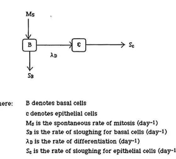
a). Spontaneous Rate of Mitosis (Ms):

The process of spontaneous mitosis in the lung occurs mainly in

the basal cells of each generation. The dividing basal cells may

either be lost by sloughing, or differentiate into epithelial cells, which

in turn may be lost by sloughing. The schematic model describing

the spontaneous mitosis of the lung is displayed in Figure 4.

The mathematical formulations are given as follows:

d NB(t)

--- = MsNB(t)-(^D+SB)NB(t) (32)

d t

Ms

M

0

kds

kRi

kos

Mb

:^

kds

kis

Ms

N/ -7 2/3

kds

k3s

M«

^ 4

kds

ͣ

>

Where: Numerical number i (i.e. o, 1, 2, 3, 4) represents state i

Ms is the spontaneous rate of mitosis (day-i)

kds is the spontaneous rate of cell killing (day-i)

k^i is the rate of cell repair from state 1 back to state 0 (day-i)

Kis is the spontaneous rate of transition for state i (day-l)

Figure 3 Model for Background Transition

Ms

Sb

^ e Ad

ͣ

> Se

Where: B denotes basal cells c denotes epithelial cells

Ms is the spontaneous rate of mitosis (day-i)

Sb is the rate of sloughing for basal cells (day-i)

Ad is the rate of differentiation (day-i)

Sc is the rate of sloughing for epithelial cells (day-i)

Figure 4 Model for Spontaneous Mitosis

d Ne(t)

--- = >.DNB(t)-Se Ne(t) (33)

d t

Assume that Ng = k Nb, which means each dividing basal cell

could differentiate into k epithelial cells. Inserting this relation into

Ms = Xd(1 + l/k) + SB-Se (34)

If k equals 1, then

Ms = 2 Xd + Sb - Se

Inserting Xd = ( Ms + Sg - Sb )/2 into equation (32) yields:

1 dNB

Ms = 2(---) + (SB + Se) (35)

Nb dt If k equals 2, then

Ms = 2 Xd/3 + Sb - Se

Inserting >,d = 2 ( Mg + Se - Sb )/3 into equation (32) yields:

1 dNB

Ms = 3(---) + (SB + Se) (36)

Nb dt

A general expression of Ms is : 1 dN

Ms=(k+1)(---) + S (37)

N dt

1 dN

Where:---is the fractional rate of change of the lung mass

N dt

S equals (Sb + kSe), which is the overall rate of

sloughing of lung cells

The value of 2 for k is employed in this study, since there are approximately two epithelial cells for each basal cell in the upper generations of the TB region. Therefore,

1 dN

Ms = 3(---) + S (38) N dt

The age dependent values of (1/N) (dN/dt) are shown in Figure 5, taken from a paper by Crawford-Brown (C-B83).

It should be noted that the curve for the whole body is used here due to the absence of data specific to lung epithelium. The age-dependent values of S are determined by the biological half-life in humans of i37Cs in the whole body. It is assumed that i37Cs js

retained in the body by attachment to biomolecules in cells. When

cells are removed, the contained i^T^g goes with them. Based on this assumption, the half-life of the ^37Cs in human bodies is considered

to be identical to the half-life for removal of cells. If the mechanism

of excretion is governed by a first-order kinetics, the relation of the half life (T1/2) and the rate of sloughing (S) is given by:

S = 0.693 / Ti/2 (39)

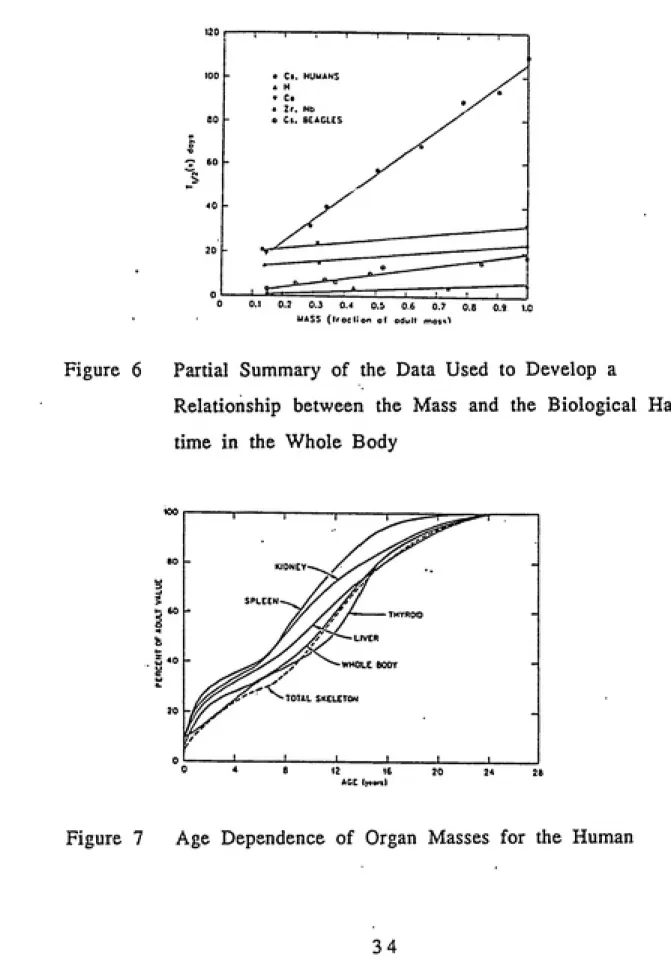
The value of T1/2 as a function of organ mass (fraction of adult

mass) may be seen from Figure 6 (C-B83). The age dependence of

organ masses in units of percent of adult value for the human may

be found in Figure 7 (C-B83). Therefore, inserting the data from

Figure 6 and Figure 7 into equation (39), the age-dependent rates of sloughing (S) can be obtained.

10"

SKtLETON

LIVER

WHOLE BODY K DNEY

SPLEEN^.

AGE (ytort)

Figure 5 Age Dependence for Fractional Rate of Change of the

120 r

« Cs. HUMANS

A H

• c.

• Zr. Nb o Ci. 8£*GLES

0.1 0.2 0.3 0.4 0.5 0.6 0.7 0.8 0.9 1.0

MASS ((roclion o( oduM mos^l

Figure 6 Partial Summary of the Data Used to Develop a

Relationship between the Mass and the Biological

KIDNEY

SPLEEN

THYROID LIVER

WHOLE BODY TOTAL SKELETON

12 16 AGE lyconl

Figure 7 Age Dependence of Organ Masses for the Human

Table 2 provides a list of the fractional rate of organ growth,

(l/N)(dN/dt), and the rate of sloughing, S, for each year prior to age

22. Beyond age 22, these rates are constant.

b). Spontaneous Rate of Transition from State 0 to State 1 (kos):

It is assumed in this analysis that kos is independent of age.

Based on the concept of material balance at equilibrium, the rate of

input must be equal to the rate of output for state 0. This

relationship, shown in Figure 3, may be formulated as follows:

Ms NoE + k^i NiE = (kds + kos) No (40)

Therefore, kos = (Ms - kds ) + k^^ (Nie/Nqe) (41)

To maintain organ homeostasis in adults, the background rates

of mitosis and cell killing are approximately equal (i.e. Ms = kds).

Therefore, the value for kos is 0.2 day-i.

The spontaneous rate of transition from state 0 to state 1, kos,

is an input for state 1. A cell in state 1 will undergo one of the

following three fates: (1) it undergoes further transition to state 2

with a rate of kis; (2) it is removed by background cell killing with a

rate of kds; or (3) it is repaired and goes back to state 0 at a rate of

R R

k 1. Due to the relatively large value of k i, the actual rate of

transition from state 0 to state 1 is significantly offset by cell repair.

Therefore, the fraction of kos that contributes to transitions is equal

to the sum of kg and kig divided by the sum of kg, kis, and k i. The

effective portion of kos, referred to as (kos)eff, is the product of kos

and the fraction of transitions (from state 0 to state 1) which avoid

repairing the cells in state 1 back to state 0. This yields :

Table 2 Age-Dependent Values for the Fractional Rate of Organ Growth (l/N)(dN/dt) and the Rate of Sloughing (S)

per year

Age fl/N) CdN/dt^

0.5

S

0 14.45

1 0.35 14.05

2 0.2 12.05

3 0.12 11.5

4 0.08 8.43

5 0.07 7.23

6 0.085 6.67

7 0.09 6.32

8 0.095 6.02

9 0.1 5.06

10 0.11 4.60

1 1 0.11 4.36

12 0.1 4.08

13 0.095 3.78

14 0.085 3.51

15 0.07 3.24

16 0.05 3.16

17 0.04 2.98

18 0.03 2.81

19 0.03 2.72

20 0.03 2.66

21 0.03 2.58

kds + kls

(kos)eff =(--- ) kos (42)

kds + kls + k^i

= 0.00638 (day-l)

= 0.23 (year-1)

In fact, ko is a function of dose rate. However, the radiation

component is relatively small compared to the background rate. It is

assumed that ko is not significantly affected by radiation and is

independent of age in this study. The constant value of 0.23 (yr'l)

derived above is applied to each age.

c). Spontaneous Rate of Transition from State 1 to State 2 (kis):

As with kos, kls is estimated at equilibrium with D equal to

kisNiE + Ms (I-P4) NsE = MSP4N3E +kdsN3E (43) Therefore, kis = [ Ms (2P4-I) + kds ] (Nbe/Nje) (44)

P4 is a constant representing the probability per cellular

division that a cell in state 3 will undergo transition to state 4. Its

value equals 5 x 10-4, which was determined by Crawford-Brown

and Hofmann (C-B90) using the data of Han et al (Han84). N3E times

P4 is the fraction of cells in state 3 undergoing transition to state 4

during mitosis, while the fraction of cells remaining in state 3 will be

equal to N3E times (I-P4). It is assumed here that Mg = kds- The

value of kls is obtained as follows :

kis=2P4Ms(N3E/NiE) (45)

= 1.67 X lO-^ (day-i)

= 0.00006 (yr-i)

d). Spontaneous Rate of Transition from State 3 to State 4 (k3s):

The transition from state 3 to state 4 is a division-related

fixation, which is proportional to the mitotic rate with a constant P4.

k3s = Ms P4 (46)

= Ms 5 X 10-4

e). Spontaneous Rate of Transition from State 4 to State 5 (k4s):

From in-vitro studies, a lifetime probability of spontaneous

promotion is determined to be approximately 0.1 (C-B90). This value

has been shown to be consistent with limited in-vivo data. Assuming

a mean life expectancy of 73 years in the U.S. and a 20-year latency

period of developing a lung cancer, the time interval for promotion

(neglecting the initiation period) to occur is about 53 years.

Therefore,

53

J k4s dt = 0.1 (47)

0

k4s = 2 X 10-3

3.2.2. Radiation Induced Rates

The value of kiR was determined from in-vitro experiments

(Roo90), and equals 4 x 10-^ mrad-1. The rate of mitosis is

stimulated by cell killing due to exposure to radiation, and the rate of

radiation induced mitosis (Mr) is assumed to equal the rate of cell

killing caused by radiation to maintain the lung mass. The value of

kdR is taken here to be 1.67 x lO'^ mrad"!.

0

The parameter k4R(D) is a radiation induced rate related to

contact inhibition removal within the cellular community during

mitosis. This depends on a specific number of dead cells surrounding

a cell in state 4. As discussed earlier, the total number of cells

contiguous to a epithelial cell is six, and at least four of these six cells

must be dead to stimulate the transition toward state 5. Assuming

binomial distribution, therefore.

x=6 x! (fy(l-f)^-'

k4R(D) = M(D)X

---i=4 (x-i)! i!

(48)

Here, f is the fraction of dead cells in the tissue surrounding a

cell in state 4. It is assumed that cells, except those being killed, are

in a dividing state. These surviving cells are removed from the

organ by lysis at rate constant R (C-B90). Therefore, f is given by the

following relationship :

kd(D)

f =--- (49)

Where R is the rate of removal set equal to 1 dayi to be

consistent with the rate of mitosis in heavily damaged organs (C-B91

in press).

A summary of parameter values used in state-vector model of

this study is provided in Table 3.

Table 3 Summary of Parameter Values Employed in State-Vector Model

PARAMETER VALUE

kiR

kdR

kN

ko

kis

k4s

NOE

NiE

N3E

P4

R 1 day 4 X 10-5 _mrad'l

1.67 X 10-5 mrad"^

0.13 hr-i

0.23 _yr-i

0.0061 _yr-i

0.002 _yr-i

0.94 0.06

0.001

5 X 10-4

IV. RESULTS

The influences of different amounts of ETS on the working level (WL) concentrations of radon progeny and the unattached fractions of RaA (fa) under various initial particle concentrations (N) are presented in Table 4. The initial particle concentrations refer to the

concentrations present before the introduction of ETS.

It is noted that there is a general tendency of increasing

working level concentration and decreasing unattached fraction of RaA with greater amounts of ETS. In addition, the presence of ETS

only slightly raises the working level concentration, with a maximum increase of a factor of two, but significantly reduces the unattached

fraction of RaA by three orders of magnitude which is the largest difference identified. Comparing 2 packs of cigarettes versus smoke

free for an initial particle concentration of lO^ cm-3, the ratio of the

WL concentration is equal to 2 (i.e. 3.78 x 10-3/L89 x 10-3), while

the ratio of the RaA unattached fraction increases to 1.45 x 10^ (i.e.

0.63/0.0044). Since the dose per inhaled atom is significantly higher for unattached progeny than for those attached, the effects of ETS are more significant when the initial aerosol concentration is as low as

Table 4 A List of the WL Concentrations of Radon Progeny and

the RaA Unattached Fractions under Each Set of

Exposure Conditions in the Home

N Amount smoked

(particles/c.c.) (packs/day)

103

WL

104

105

106

0 1.89 X 10-3 0.63

1/2 3.73 X 10-3 0.0172

1 3.76 X 10-3 0.0087

2 3.78 X 10-3 0.0044

0 3.29 X 10-3 0.15

1/2 3.74 X 10-3 0.0158

1 3.77 X 10-3 0.0084

2 3.78 X 10-3 0.0043

0 3.73 X 10-3 0.017

1/2 3.76 X 10-3 0.0088

1 3.78 X 10-3 0.006

2 3.78 X 10-3 0.0035

0 3.79 X 10-3 0.0018

1/2 3.79 X 10-3 0.0016

1 3.79 X 10-3 0.0015

2 3.81 X 10-3 0.0013

The calculation of annual doses for different ages with different

amounts of smoke in the environment are shown in tables 5 to 8

under each set of initial aerosol concentrations.

From the results shown in Tables 5 to 8, the addition of ETS

tends to lower the doses of radon progeny to the lung, and an

increased amount of smoke in the environment results in a lower

dose. This implies that when the initial concentration is so high that almost all the progeny have been attached to particles, the contribution of aerosol particles from ETS has a minimal effect on the calculated progeny doses. In addition, the curve of age-variant doses reveals that the subgroup most sensitive to radon progeny exposure would be children in the ages between 5 and 10.

It is interesting that the doses with ETS present are slightly

higher for Ni = lO^ cm-3 than those corresponding doses for Nj = 10^ cm-3 regardless of age and amounts of cigarette smoke. The similar

relationship remains for the case of comparing the doses when Ni

raises from 10^ up to 10^ cm-3. But, for the case of comparing the

doses for Ni = 10^ and 10^ cm-3, a decreasing tendency of annual

complicated process of dose calculation, it is difficult to pinpoint out a specific factor responsible for this change. Instead of comparing the

doses among different values of Ni, however, a comparison concerning the relative change of annual doses with and without ETS

present for each initial aerosol concentration may provide an indirect

The value of RaA unattached fraction (fa) for Ni = 10^ cm-3

without ETS present is approximately four times of that for Ni = 10^

ETS, which will release an amount of particles equal to a magnitude

of five orders per cm3 into the ambient air, reduces the f^ down to

approximately the same level for both Ni = 103 and 10^ cm"3. For all

ages, the addition of ETS equal to 1/2 pack of cigarettes per day

lowers the doses by a factor of four for Ni = 103 cm-3 and by a factor

particles that have more significant effect on reducing the RaA

unattached fraction for Ni = 103 cm-3 than that for Ni = 10^ cm-3.

The final sensitivity analysis for life-time relative risk of lung

cancer (i, e. the possibility of lung cancer with ETS present compared

to that without ETS present) is displayed in Table 9.

If the initial aerosol concentration in the home is less than 10"*

cm-3, the addition of ETS equal to less than 1 pack of cigarettes per

day may lower the risk of lung cancer. A general trend indicates

that the relative risk of lung cancer increases as the initial concentration goes up and more ETS is added.

Table 5 Annual Irradiation Doses for Different Ages and Various Levels of ETS Present with Initial Aerosol Particles Equal

to 103 cm-3

Age

(yrs)

Annual Doses (mrad/year), when Ni= 103 |

Amount Smoked (packs) |

0 1/2 1

2 1

0 ₂₆₀ 70 _{65 65}

2 ₂₅₀ 63 56 56

5 320 60 75

75 1

10 340 65 79

79 1

22 150 36 35

35 1

Table 6 Annual Irradiation Doses for Different Ages and Various

Levels of ETS Present with Initial Aerosol Particles Equal

to 104 cm-3

Age

(yrs)

Annual Doses (mrad/year), when Ni= 104 |

Amount Smoked (packs)

0 1/2 1

2 1

0 220 64 60

60 1

2 200 11 ₇₃ 73

5 250 96 91

91 1

10 270 102 ₉₆ 96

22 120 46 44

44 1

Table 7 Annual Irradiation Doses for Different Ages and Various

Levels of ETS Present with Initial Aerosol Particles Equal

to 105 cm-3

Age

(yrs)

Annual Doses (mrad/year), when Ni= 105

Amount Smoked (packs)

0 _1/2 1 2

0 77 61 61 61

2 70 _{56 56 56}

5 66 70 70 70

10 ₉₅ 76 _{76 76}

22 42 _{34 34}

34

Table 8 Annual Irradiation Doses for Different Ages and Various

Levels of ETS Present with Initial Aerosol Particles Equal

to 105 cm-3

Age

(yrs)

Annual Doses (mrad/year), v/hen Ni= 106

Amount Smoked (packs)

0 _{1/2 1 2}

0 66 66 66 66

2 60 60 _{60 60}

5 75 75 75 75

10 _{61 61}

61 61

22 _{36 36}

36 36

Table 9 Life-time Relative Risks of Lung Cancer under Each Set of Exposure Conditions in the Home

Initial Aerosol

Concentration

(particles/cm3)

RRETS/vithoutETS

1/2 packs of

cigarettes

of ETS

1 pack of cigarettes

of ETS

2 packs of cigarettes

of ETS

103 _0.693 0.766 1.000

104 0.601 0.669 1.164

105 1.060 _1.193 1-560

106 1.115 1.255 1.641

DISCUSSION

The analysis in Table 9 implies that estimating the possibility

of lung cancer depends on various competing factors. The initial

aerosol concentration in the home plays an important role in

quantifying the effect of ETS on radon exposure.

For relatively low concentrations of aerosol particles (less than

lO^cm'^), the presence of ETS lowers the unattached fraction of RaA

and progeny doses dramatically. This may result in a lower risk of

lung cancer than a smoke free environment. Combining the

promotional effect of ETS by an increased risk of 2.4 % per pack of

cigarettes, the final results indicate a decreased relative risk of 0.766

for an initial particle concentration of 10^ cm-3, and 0.889 for an

initial particle concentration of lO^cm-3. Analogously, the smoke

from 1/2 pack of cigarettes will result in a decreased relative risk of

0.693 for an initial particle concentration of 10^ cm"3, and 0.801 for

an initial particle concentration of 10^ cm-3.

It is noted that the influence of ETS on radon induced lung

cancer is related to, but not limited to, the competition of the initial

aerosol concentration and the magnitude of promotional effect of ETS.

For low initial aerosol concentrations in the home, the particle

density in air has a dominating effect on progeny attachment and

will yield a relatively lower risk of lung cancer; however, for high

-umt' "'" muv^mfi

initial aerosol concentrations, the promotional effect outweighs the

reduced radiation dose due to the addition of ETS. This will result in

a higher risk of lung cancer.

The results predicted from this study are basically consistent with the results from animal experiments. The NRC report (NRC88)

found that respiratory tract tumor incidences

* increase with the unattached fraction of radon progeny.

* decrease if cigarette smoking follows completion of exposure to radon progeny, but has no effect if smoking precedes exposure.

* decrease if animals are exposed to smoking and radon progeny alternately on the same day.

The combined lung cancer relative risk of 1.34 from the meta¬ analysis of 13 epidemiological studies (NRC86) is much higher than would be expected from comparisons of biological markers of smoke exposure between ETS-exposed people and active smokers. The analysis of urinary levels of cotinine discussed in the NRC report (NRC86) suggested that ETS exposure was roughly equivalent to smoking 0.1 to 0.2 cigarettes per day, which is approximately the

range used in the present study (i.e. 0.04 to 0.16 cigarettes per day). The excess lung cancer risk calculated from epidemiological studies (34%) is about 10 times greater than the excess lung cancer risk

obtained here using extrapolation from MS smoke data to estimate

the cigarette equivalence inhaled by the passive smoker (1.2 to 4.8%). The NRC contended that the effects of ETS cannot be precisely

compared on the basis of biological markers due to the different

components between ETS and MS smoke. Another explanation from

the opposite viewpoint stated that the observed association from

epidemiological studies was misclassification of smokers and

ex-smokers as nonex-smokers. This discrepancy raises the controversy of

the association between ETS and lung cancer remained to be further

identified.

The most striking conclusion of this study suggests that the effect of ETS on radon-induced lung cancer can not be simply

classified as protective, additive, or synergistic. Whether the

combined risk is less than, equal to, or greater than these two

separate risks primarily depends on the initial aerosol concentration

and the amounts of ETS in the home. Several competing factors

influence the effect of ETS on radon progeny, which complicates the

mitigation schemes.

For the initial particle concentration of 10^ or 10^ cm-3 and the

lung cancer. A higher risk is computed in this study. When the

initial particle concentration exceeds 10^ cm-^, the removal of ETS