Vol. 3, No. 2, pp 251-270
Periodic Oscillations in the Analysis of
Algorithms and Their Cancellations
Helmut Prodinger∗
The John Knopfmacher Centre for Applicable Analysis and Number The-ory, School of Mathematics, University of the Witwatersrand, Private Bag 3, Wits, 2050 Johannesburg, South Africa. ([email protected])
Abstract. A large number of results in analysis of algorithms con-tain fluctuations. A typical result might read “The expected number of . . . for large n behaves like log2n+ constant +δ(log2n), where
δ(x) is a periodic function of period one and mean zero.” Examples include various trie parameters, approximate counting, probabilistic counting, radix exchange sort, leader election, skip lists, adaptive sampling. Often, there are huge cancellations to be noted, espe-cially if one wants to compute variances. In order to see this, one needs identities for the Fourier coefficients of the periodic functions involved. There are several methods to derive such identities, which belong to the realm of modular functions. The most flexible method seems to be the calculus of residues. In some situations, Mellin trans-forms help. Often, known identities can be employed. This survey shows the various techniques by elaborating on the most important examples from the literature.
∗
Supported by NRF Grant 2053748.
Received: October 2003, Revised: March 2004
Key words and phrases: Analysis of algorithms, approximate counting, Dedekind’s eta function, geometric random variables, Mellin transform, modu-lar functions, periodic oscillations, residues, tries.
1
Introduction
A surprisingly large number of results inanalysis of algorithms con-tainfluctuations. A typical result might read “The expected number of . . . for large n behaves like log2n+ constant + δ(log2n), where
δ(x) is a periodic function of period one and mean zero.” Examples include various trie parameters, approximate counting, probabilis-tic counting, radix exchange sort, leader election, skip lists, adap-tive sampling; see the classic books by Flajolet, Knuth, Mahmoud, Sedgewick, Szpankowki [23, 16, 17, 18, 25] for background.
We use the name δ(x) in a generic sense; in concrete situations we call them δ0(x),δ1(x), etc. An important set of such functions is
δj(x) :=
1
L
X
k6=0
Γ(j−χk)
j! e 2πikx,
where we use the standard abbreviations L= log 2 and χk= 2πikL .
Figure 1: δ0(x) and δ02(x)
As one can see from the picture, δ0(x) has mean zero (the zeroth Fourier coefficient is not there). On the other hand, δ20(x) is still periodic with period 1, but its mean is not zero. Why should we worry about a quantity apparently as small as≈10−12?
The reason is the variance of such parameters, as it naturally contains the term “−expectation2,” and as such also −δ2(x). That might not be a sufficient motivation for a casual reader if it were not the case that often substantial cancellations occur. In order to identify them, one has to know more about δ2(x). If one ignores these terms, one gets wrong results, and the results are not wrong by
≈ 10−12, but by an order of growth! Path length in tries, Patricia –1.5e–06
–1e–06 –5e–07 0 5e–07 1e–06 1.5e–06
–2 –1 1 2
x
5e–13 1e–12 1.5e–12 2e–12 2.5e–12
–2 –1 1 2
x
Figure 2: The functions δj(x) = L1 Pk6=0
Γ(j−χk)
j! e
2πikx grow in
am-plitude
tries, and digital search trees [8, 15, 10] are such cases: the variance is in reality of ordern only, but ignoring the fluctuations would lead to a (wrong) ≈n2 result.
Questions like that occurred in several writings of this author (together with various coauthors), as can be seen from the references. The techniques are extremely interesting, as one has to dig deep into classical analysis. So far, it seems that the calculus of residues is the most versatile approach in this context. Another approach is to use (modular) identities due to Dedekind, Ramanujan, Jacobi and others (which can often be proved by Mellin transform techniques); however, often they do not quite fit. The residue calculus approach directly addresses the formula that is ultimately needed.
In this survey paper, we discuss all these methods by looking at various examples. The paper has also a tutorial concern, as we want to encourage the interested reader to prove his/her own identities with the methods that are provided.
Oscillating functions are usually given as Fourier series f =
P
k6=0ake2πikx, thus representing a periodic function of period 1, and
since the term a0 is missing, oscillating around zero. We often refer to the coefficient ak by writing [f]k.
Other cancellation phenomena concerning oscillations related to Patricia tries and compositions (resp. words) were only discovered recently and presented in [22], at analco04 (dedicated to Hosam
Mahmoud).
Here are some examples from the literature. –0.0002
–0.0001 0 0.0001 0.0002
–2 –1 1 2
x
Approximate counting [5, 11, 20, 21]
After nsuccessive increments the average content Cn of the counter
satisfies:
Cn∼log2n+
γ
L−α+
1
2−δ0(log2n), with
α=X
k≥1 1
2k−1 and δ0(x) =
1
L
X
k6=0
Γ(−χk)e2πikx,
withL= log 2 and χk= 2πikL . The identity that one needs is
[δ02]0 = 1
L2
X
k6=0
Γ(χk)Γ(−χk) =
π2
6L2 − 11 12 −
2
L
X
h≥1
(−1)h−1
h(2h−1). (1)
We will present various proofs of this identity, which will be our running example, in the next sections. The methods are residue calculus (Section 2), Mellin transform (Section 3), and identities of Ramanujan (Section 4).
Maximum of a sample of n geometric random variables [26, 13]
Assume thatXis a geometric random variable such thatP{X=k}=
2−k (for simplicity, we only discuss this case, not the slightly more general P{X =k}= (1−q)qk−1). We considern independent trials
and look for their maximum. This is a natural parameter which is also useful in the analysis of various algorithms (e. g., skiplists [14]).
The expected value is given by
En∼log2n+
γ L +
1
2 −δ0(log2n) with the same periodic function as before.
Tries [12, 8, 7]
The expected number of internal nodes in a trie built fromnrandom data is
ln=
n
L+nσ(log2n) +O(1),
with
σ(x) = 1
L
X
k6=0
χkΓ(1−χk)e2πikx.
The formula that one needs is [σ2]0 = 3− 1
L −
1
L2 + 2
L
X
j≥2
(−1)jj
(j+ 1)(j−1)(2j −1). (2)
Partial match queries in tries [9]
The average cost (defined in the paper [9]), for random tries con-structed fromn random data, is
ln=
√
n√π1 + √
2
2L +τ log2 √
n+O(1),
where the fluctuating functionτ(x) =P
k6=0τke2kπix has the Fourier
coefficients
τk=
1 2L
1 +√2(−1)kΓ−1−χk 2
−1 +χk
2
.
The formula one needs is [τ2]0 = 3
4L − π
4L2 3 + 2
√
2+3−2
√
2
L F(L) +
2√2
L F
L
2
(3) with
F(x) =X
k≥1
e−kx
1 +e−2kx.
2
Proofs by residue calculus
In this section we will show how to use residue calculus in order to prove the relevant identities. As examples of the technique, we concentrate on the identities (1), (2), and (4). However, after going through these representative examples, the reader will surely be able to prove his/her own identities, following the technique.
The following approach (“residue calculus”) to evaluate [δ2]0seems to be the easiest and most flexible. We start with the following ex-ample:
δ0(x) = 1
L
X
k6=0
Γ(−χk)e2πikx.
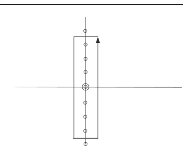
Figure 3: Path of integration; poles at χk are indicated, the double
pole at 0 by a double circle
Find a functionF(z) so that [δ02]0 is (apart from a few extra terms) the sum of the residues along the imaginary axis. Here, take
F(z) = L
eLz−1Γ(−z)Γ(z).
If we set
I1 = 1 2πi
Z 1
2+i∞ 1 2−i∞
F(z)dz,
then by shifting and collecting residues,
I1= 1 2πi
Z −1
2+i∞ −1
2−i∞
F(z)dz+X
k6=0
Γ(−χk)Γ(χk)−
π2
6 −
L2
12. What happens here is often called closing the box, compare Fig-ure 3, see e. g. [25, 18]. One integrates along a rectangle with corners
±1
2 ±iM. One can evaluate it by collecting the residues inside the rectangle. And one can let the parameter M go to infinity. In this type of problems, the integrals along the horizontal lines disappear, and we can express one integral along a vertical line by an integral along another vertical line, plus a few residues. The justification that these integrals along the horizontal lines disappear comes from the fact that the Gamma function (which is always present in our ex-amples) becames small extremely fast for large imaginary parts, see [27]. Since all our examples are of that nature, we will perform the relevant operations without further comments.
The emphasis of this survey is to prove identities, and this is to some extent a more algebraic than analytic endeavour.—
Now one writes
1
ez−1 =−1−
1
e−z−1
and gets, by a simple change of variable z:=−z,
I1 =− 1 2πi
Z −1
2+i∞ −1
2−i∞
Γ(−z)Γ(z)dz−I1+
X
k6=0
Γ(−χk)Γ(χk)−
π2 6 −
L2 12. The integral
I2 =− 1 2πi
Z −1
2+i∞ −1
2−i∞
Γ(−z)Γ(z)dz
can be computed by collecting the negative residues right to the line
<z=−12, viz.
I2 =− 1 2πi
Z −1
2+i∞ −1
2−i∞
Γ(−z)Γ(z)dz=X
l≥1 (−1)l
l! (l−1)! =−L. Altogether we have
2I1 =−L+
X
k6=0
Γ(−χk)Γ(χk)−
π2
6 −
L2
12.
On the other hand, integralI1 is also the sum of the negative residues right of the line<z= 12, i. e.,
I1 =−L
X
l≥1
(−1)l
l!(2l−1)(l−1)! =−L X
l≥1
(−1)l
l(2l−1).
Combining these results, we get
−2LX
l≥1
(−1)l
l(2l−1) =−L+ X
k6=0
Γ(−χk)Γ(χk)−
π2
6 −
L2
12. This is the identity we wanted.
With not much more effort one can also compute the coefficients [δ20]k, fork6= 0. For this, one works with the function
F(z) = L
eLz−1Γ(−z−χk)Γ(z).
One obtains [δ20]k= 1
L2
X
j6=0,6=k
Γ(−χj)Γ(−χk+χj)
= 2
L
X
l≥1
(−1)lΓ(−χk+l)
l!(2l−1) +
2
L2Γ(−χk) ψ(−χk) +γ
.
We omit the details.
Guy Louchard, who is interested in higher moments, asked to compute the coefficients [δ30]k. Here is the instancek= 0, the general case is very involved and not too attractive:
[δ30]0 =−1− 2ζ(3) L3 −
1
L
X
l≥1
(−1)l
l(2l−1)+
6
L2
X
l≥1
(−1)lHl−1
l(2l−1) +
2 log 3
L
+ 2
L
X
l,j≥1
(−1)l+j (l+j)(2l−1)
1 2j −1 +
1 2j+l−1
l+j j
.
(In this formula, the harmonic numbersHn:=P1≤k≤n1k appear.)
This has been tested numerically as well and gives 9.42817763095796606421903×10⁻²⁵.
Let us straight ahead do another example (identity (2)), which also occurs often:
σ(x) = 1
L
X
k6=0
χkΓ(−1−χk)e2πikx.
Here, we take
F(z) =− L eLz−1z
2Γ(−1−z)Γ(−1 +z).
Then
I1= 1 2πi
Z −1
2+i∞ −1
2−i∞
F(z)dz+X
k6=0
χk(−χk)Γ(−1−χk)Γ(−1 +χk) + 1
and
2I1 =LI2+
X
k6=0
χk(−χk)Γ(−1−χk)Γ(−1 +χk) + 1
with
I2 = 1 2πi
Z −1
2+i∞ −1
2−i∞
z2Γ(−1−z)Γ(−1 +z)dz
=X
l≥2
l2(−1)
l+1
(l+ 1)!(l−2)! +
L
4
=X
l≥2
(−1)l+1l
(l+ 1)(l−1) =−L+ 1 4+
1
4 =−L+ 1 2. Therefore
2I1 =−L2+
L
2 +
X
k6=0
χk(−χk)Γ(−1−χk)Γ(−1 +χk) + 1.
But I1 is also
I1=−
L
4 +L
2+LX l≥2
l2
2l−1
(−1)l+1
(l+ 1)!(l−2)! =−L
4 +L
2+LX l≥2
(−1)l+1l
(2l−1)(l+ 1)(l−1).
Putting things together, we find 2I1 =−L2+
L
2 +
X
k6=0
χk(−χk)Γ(−1−χk)Γ(−1 +χk)
=−L
2 + 2L
2+ 2LX l≥2
(−1)l+1l
(2l−1)(l+ 1)(l−1)+ 1,
or
X
k6=0
χk(−χk)Γ(−1−χk)Γ(−1 +χk)
=−1−L+ 3L2+ 2LX
l≥2
(−1)l+1l
(2l−1)(l+ 1)(l−1),
which is the identity in question, as it expresses the quantity L2[σ2] 0 in two different ways.
Here is a third example, dealing with the function 1
L
X
k6=0
Γ(j−χk)e2πikx,
for j ≥ 1, and the computation of the constant term of its square. The technique should be familiar by now. Consider the function
LΓ(j+z)Γ(j−z) eLz−1 .
Therefore we have
X
k6=0
Γ(j+χk)Γ(j−χk) =
L
2πi
Z 12+i∞
1 2−i∞
Γ(j+z)Γ(j−z)
eLz−1 dz
− L
2πi
Z −1
2+i∞ −12−i∞
Γ(j+z)Γ(j−z)
eLz−1 dz−Γ(j)
2.
(Γ(j)2 is the residue atz= 0.)
Now we use again the decomposition 1
eLz−1 =−1−
1
e−Lz−1
for the second integral and get
− L
2πi
Z −1
2+i∞ −1
2−i∞
Γ(j+z)Γ(j−z)
eLz−1 dz
= L
2πi
Z −1
2+i∞ −1
2−i∞
Γ(j+z)Γ(j−z)dz
+ L
2πi
Z −1
2+i∞ −1
2−i∞
Γ(j+z)Γ(j−z)
e−Lz−1 dz
= L
2πi
Z i∞
−i∞
Γ(j+z)Γ(j−z)dz
+ L
2πi
Z 1
2+i∞ 1 2−i∞
Γ(j−z)Γ(j+z)
eLz−1 dz.
Therefore
X
k6=0
Γ(j+χk)
2
= 2L 2πi
Z 12+i∞
1 2−i∞
Γ(j+z)Γ(j−z)
eLz−1 dz
+ L
2πi
Z i∞
−i∞
Γ(j+z)Γ(j−z)dz−Γ(j)2
=I1+I2−Γ(j)2.
IntegralI1 is evaluated by shifting the contour to the right and col-lecting the negative residues, which gives
I1=−2L
X
m≥j
Γ(j+m)
eLm−1
(−1)j−m+1 (m−j)! and withm=h+j
= 2LX
h≥0
(h+ 2j−1)!(−1)h
h!
1 2h+j−1
= 2L(2j−1)!X
h≥0
−
2j h
1 2h+j−1.
IntegralI2 is of interest for itself and appears already in early ref-erences to the Mellin transform technique as by Nielsen [19, p. 224]. (It could, however, by computed as in the previous examples.)
We start with the function
f(x) = x
j
(1 +x)2j
and perform its Mellin transform (see, e.g., [6] for definitions)
f∗(s) =
Z ∞
0
f(x)xs−1dx=B(j+s, j−s) = Γ(j+s)Γ(j−s) Γ(2j)
with the Beta functionB(z, w) (compare [1]). The fundamental strip
is h−j, ji. Therefore the inversion formula for the Mellin transform gives
f(x) = 1 2πi
Z i∞
−i∞
Γ(j+s)Γ(j−s) Γ(2j) x
−sds.
Now we may evaluate at x= 1 and get the formula 1
2πi
Z i∞
−i∞
Γ(j+s)Γ(j−s)ds= Γ(2j)2−2j.
This produces the formula
X
k6=0
Γ(j+χk)Γ(j−χk)
= 2L(2j−1)!X
h≥0
−2j h
1
2h+j −1 +L(2j−1)!2
−2j−(j−1)!2.
(4) This formula was essential in the paper [13].
Remark. The computation of the integral I2 (as in the examples above) sometimes leads to series like
X
l≥1
(−1)ll.
There is nothing wrong here. The correct interpretation is as anAbel limit
lim
t→1−
X
l≥1
(−1)lltl= lim
t→1− −t
(1 +t)2 =− 1 4.
3
Using the Mellin transform to prove
iden-tities
Let us start with our running example (1) and show how this can be proved using the Mellin transform. The Mellin transform is very prominent in the analysis of algorithms, and we refer to [6] for a nice survey.
We will treat again our identity (1) and might for instance start with the series
X
h≥1
(−1)h−1
h(2h−1)
and interpret it asg(log 2) with
g(x) :=X
h≥1
(−1)h−1
h(ehx−1) = X
h,k≥1
(−1)h−1
h e −hkx.
Now one computes the Mellin transform g∗(s):
g∗(s) = X
h,k≥1
(−1)h−1
h e
−hkx = X h,k≥1
(−1)h−1
h h
−sk−sΓ(s)
= (1−2−s)ζ(s+ 1)ζ(s)Γ(s).
The Mellin transform exists in the fundamental striph1,∞i; whence we can invoke the inversion formula for the Mellin transform. We may choose e. g. the line <z = 32 since 32 lies in the fundamental strip. So we get
g(x) = 1 2πi
Z 3
2+i∞ 3 2−i∞
(1−2−s)ζ(s+ 1)ζ(s)Γ(s)x−sds
= π 2 12x −
L 2 + x 24 + 1 2πi
Z −32+i∞
−3 2−i∞
(1−2−s)ζ(s+ 1)ζ(s)Γ(s)x−sds
= π 2 12x −
L 2 + x 24 + 1 2πi −3
2+i∞
Z
−32−i∞
(2s−1)ζ(s+ 1)ζ(s) 1 2√πΓ
s
2
Γ
s+ 1
2
x−sds.
This form was obtained by taking 3 residues out and invoking the duplication formula of the Γ-function. (Observe that the exponential smallness of the Γ-function along vertical lines justifies the shifting of the line integral.) We now use the functional equation for ζ(s), namely
Γs 2
ζ(s) =πs−12Γ
1−s
2
ζ(1−s), (5) and continue:
g(x) = π 2 12x −
L 2 + x 24 + 1 2πi
−32+i∞
Z
−3 2−i∞
(2s−1)1 2π
2s−12Γ1−s
2
ζ(1−s)Γ
−s
2
ζ(−s)x−sds
= π 2 12x −
L 2 + x 24 + 1 2πi Z 3
2+i∞ 3 2−i∞
(2−s−1)1 2π
−2s−1 2Γ
1 +s
2
ζ(1 +s)Γ
s
2
ζ(s)xsds
= π 2 12x −
L 2 + x 24 − 1 2πi Z 3
2+i∞ 3 2−i∞
(1−2−s)π−2sζ(1 +s)ζ(s)Γ(s)xs2−sds,
and so
g(x) = π 2 12x −
L
2 +
x
24 −g
2π2
x
. (6)
This is the formula we need, since we can also rewrite the left side of (1) in terms of this g(x) function:
[δ20]0 = 1
L2
X
k6=0
Γ(χk)Γ(−χk)
= 1
L
X
k≥1
1
ksinh(2kπ2/L) = 2
L
X
k≥1
ekz
k(e2kz−1),
withz= 2π2/L. But
X
k≥1
ekz k(e2kz−1) =
X
k≥1, j≥0 1
ke
−k(2j+1)z
= X
k≥1, j≥1 1
ke
−kjz−2 X k≥1, j≥1
1 2ke
−2kjz
= X
k≥1, j≥1
(−1)k−1
k e
−kjz=X k≥1
(−1)k−1
k(ekz−1) =g(z),
and so
[δ20]0 = 2
Lg
2π2
L
.
Let us do a more complicated example in the same style: We want to rewrite [τ2]0, to get identity (3). Note that
[τ2]0 = 2X
k≥1
τkτ−k =
2 4L2
X
k≥1
3 + 2√2(−1)kΓ1−χk 2
Γ1 +χk 2
.
Now we use the formula (equivalent to the reflection formula for the Gamma function, cf. [1]) Γ(z)Γ(1−z) =π/sinπz and obtain
Γ
1−χk
2
Γ
1 +χk
2
= π
sin(π/2 +ikπ2/L) =
π
cos(ikπ2/L)
= π
cosh(kπ2/L) = 2π
e−kπ2/L
1 +e−2kπ2/L,
so that
[τ2]0 = π
L2
X
k≥1
3 + 2
√
2(−1)k
e−kπ
2/L
1 +e−2kπ2/L. (7)
Let us define two new functions
F(x) =X
k≥1
e−kx
1 +e−2kx and G(x) = X
k≥1
(−1)k−1e−kx
1 +e−2kx .
Then, (7) in terms ofF(x) andG(x) becomes
[τ2]0= 3π
L2F
π2
L
−2 √
2π L2 G
π2
L
. (8)
We use a series transformation for F(x) and G(x). We start with
F(x) =X
j≥0
(−1)jX
k≥1
e−k(2j+1)x=X
j≥0
χ(j) 1
ejx−1
where
χ(j) =
0, forj even; 1, forj≡1 mod 4;
−1, forj≡3 mod 4.
Once we know that
F(x) = π 4x −
1 4+
π xF
π2
x
, (9)
forx >0, as we shall show soon, then G(x) =F(x)−2F(2x), hence
G(x) = 1 4+
π xF
π2
x
−π xF
π2
2x
.
Applying the above to (8) we finally obtain
[τ2]0 = 3 4L −
π
4L2 3 + 2
√
2+3−2
√
2
L F(L) +
2√2
L F
L
2
.
To prove (9) we proceed as follows. Let
β(s) =X
j≥0
(−1)j 1 (2j+ 1)s.
We have
F(x) =X
k≥1
e−kx
1 +e−2kx = X
j≥0
(−1)jX
k≥1
e−k(2j+1)x,
so that the Mellin transform F∗(s) = R∞
0 F(x)x
s−1dx of F(x) be-comes F∗(s) = Γ(s)ζ(s)β(s). By the Mellin inversion formula this yields
F(x) = 1 2πi
Z 3
2+i∞ 3 2−i∞
Γ(s)ζ(s)β(s)x−sds.
Now we take the two residues s = 1 and s= 0 out from the above integral (observe thatβ(0) = 1/2 and β(1) =π/4, cf. [1]) and apply the duplication formula for Γ(s) to obtain
F(x) = π 4x−
1 4+
1 2πi
Z −12+i∞
−1 2−i∞
1
√ π2
s−1Γs 2
Γs+ 1 2
x−sζ(s)β(s)ds.
We now use the functional equations for ζ(s) and β(s), namely Γs
2
ζ(s) =πs−12Γ
1−s
2
ζ(1−s) and
β(1−s)Γ1− s
2
= 22s−1π−s+12Γ
s+ 1
2
β(s).
The first identity is Riemann’s functional equation for ζ(s), and the second is an immediate consequence of the functional equation for Hurwitz’sζ-functionζ(s, a) (cf. [2]), and the fact that
β(s) = 4−s
h
ζ s,14−ζ s,34
i
.
Substituting 1−s=u, we get
F(x) = π 4x−
1 4+
1 2πi
Z 3
2+i∞ 3 2−i∞
π1−2uΓ(u)xu−1ζ(u)β(u)du,
which proves (9).
Using the above scheme, several other identities which one needs in the analysis of algorithms can be proved. We refer to Szpankowski’s book [25].
4
Modular identities
Formulæ like (6) belong to the realm of modular functions. Many of them can be found in the literature, and are due to Jacobi, Dedekind,
Ramanujan and others. Berndt’s book [4] contains a wealth of infor-mation about the subject, compare also [3].
Here is a little bit of background: Let H be the upper complex halfplane{z∈C| =z >0}. Then the Dedekind ηfunction is defined
by
η(τ) =eπiτ /12Y
n≥1
1−e2πinτ, τ ∈H;
there is a transformation formula:
η−1 τ
= (−iτ)1/2η(τ).
C. L. Siegel [24] gave an elegant proof of this transformation for-mula using residue calculus.
Ramanujan considered series
f(z) :=X
k≥1
km
e2kz−1, m an odd integer,
and could relate them to f(π2/z). For the reader’s convenience, we give these formulæ here:
Set m= 2N + 1 andN ∈N,α, β >0, andαβ=π2, then
α−N
1
2ζ(2N + 1) +
X
k≥1
k−2N−1 e2αk−1
= (−β)−N
1
2ζ(2N + 1) +
X
k≥1
k−2N−1
e2βk−1
−22N
N+1
X
k=0
(−1)k B2k (2k)!
B2N+2−2k
(2N+ 2−2k)!α
N+1−kβk
(this covers the exponents −3,−5, . . .); the Bk’s are the Bernoulli
numbers. Then
X
k≥1 1
k(e2αk−1)−
1
4logα+
α
12 =
X
k≥1 1
k(e2βk−1)−
1
4logβ+
β
12, which covers the exponent−1. Furthermore,
αX
k≥1
k
e2αk−1 +β X
k≥1
k e2βk−1 =
α+β
24 −
1 4
which covers the exponent 1, and finally for N ≥2,
αNX
k≥1
k2N−1
e2αk−1 −(−β)
NX
k≥1
k2N−1
e2βk−1 = α
N −(−β)NB2N
4N ,
which covers the exponents 3,5, . . ..
The instancem=−1 is equivalent to the functional equation for Dedekind’s eta function.
References
[1] Abramowitz, M. and Stegun, I. A. (1964), Handbook of Mathe-matical Functions. Dover, 1973 A reprint of the tenth National Bureau of Standards edition.
[2] Apostol, T. (1976), Introduction to Analytical Number Theory. Springer-Verlag.
[3] Apostol, T. (1978), Modular Functions and Dirichlet Series in Number Theory. Springer-Verlag.
[4] Berndt, B. (1989), Ramanujan’s Notebooks. Part II, Springer-Verlag.
[5] Flajolet, P. (1985), Approximate counting: A detailed analysis. BIT,25, 113–134.
[6] Flajolet, P., Gourdon, X., and Dumas, P. (1995), Mellin trans-forms and asymptotics: Harmonic sums. Theoretical Computer Science,144, 3–58.
[7] Jacquet, P. and R´egnier, M. (1989), New results on the size of tries. IEEE Transactions on Information Theory,35, 203–205. [8] Kirschenhofer, P., Prodinger, H., and Szpankowski, W. (1989),
On the variance of the external path length in a symmetric dig-ital trie. Discrete Applied Mathematics,25, 129–143.
[9] Kirschenhofer, P., Prodinger, H., and Szpankowski, W. (1993), Multidimensional digital searching and some new parameters in tries. International Journal of Foundations of Computer Science,
4, 69–84.
[10] Kirschenhofer, P., Prodinger, H., and Szpankowski, W. (1994), Digital search trees again revisited: The internal path length perspective. SIAM Journal on Computing,23, 598–616.
[11] Kirschenhofer, P. and Prodinger, H. (1991), Approximate count-ing: An alternative approach. RAIRO Theoretical Informatics and Applications,25, 43–48.
[12] Kirschenhofer, P. and Prodinger, H. (1991), On some applica-tions of formulæ of Ramanujan in the analysis of algorithms. Mathematika,38, 14–33.
[13] Kirschenhofer, P. and Prodinger, H. (1993), A result in order statistics related to probabilistic counting. Computing, 51, 15– 27.
[14] Kirschenhofer, P. and Prodinger, H. (1994), The path length of random skip lists. Acta Informatica, 31, 775–792.
[15] Kirschenhofer, P., Prodinger, H., and Szpankowski, W. (1989), On the balance property of Patricia tries: External path length viewpoint. Theoretical Computer Science,68, 1–17.
[16] Knuth, D. E. (1997), The Art of Computer Programming. Vol. 1: Fundamental Algorithms, Third ed. Reading, Massachussetts: Addison-Wesley.
[17] Knuth, D. E. (1998), The Art of Computer Programming. Vol. 3: Sorting and Searching, 2nd ed. Reading, Massachessetts: Addison-Wesley.
[18] Mahmoud, H. M. (1992), Evolution of Random Search Trees. New York: John Wiley & Sons.
[19] Nielsen, N. (1906), Handbuch der Theorie der Gammafunktion. Teubner.
[20] Prodinger, H. (1992), Hypothetic analyses: Approximate count-ing in the style of Knuth, path length in the style of Flajolet. Theoretical Computer Science,100, 243–251.
[21] Prodinger, H. (1994), Approximate counting via Euler trans-form. Mathematica Slovaka,44, 569–574.
[22] Prodinger, H. (2004), Compositions and Patricia tries: No fluc-tuations in the variance! Proceedings of the 6th Workshop on ALENEX and the 1st workshop on ANALCO, L. Arge, G. Ital-iano, R. Sedgewick (Ed.), SIAM. 211–215.
[23] Sedgewick, R. and Flajolet, P. (1996), An Introduction to the Analysis of Algorithms. Reading, Massachessetts: Addison-Wesley.
[24] Siegel, C. L. (1954), A simple proof of η(−1/τ) = η(τ)pτ /i. Mathematika,1, 4.
[25] Szpankowski, W. (2001), Average case analysis of algorithms on sequences. New York: Wiley-Interscience.
[26] Szpankowski, W. and Rego, V. (1990), Yet another application of a binomial recurrence: Order statistics. Computing,43, 401– 410.
[27] Whittaker, E. T. and Watson, G. N. (1927), A Course of Modern Analysis. Fourth edition, Cambridge University Press, Reprinted 1973.