Volume 05 Issue 01: (2018) Jan. 2018

(1)

ISSN: 2349-4468

International Journal of Advances in Management, Economics and

Entrepreneurship

Available online at:

www.ijamee.info

RESEARCH ARTICLE

Causes of Poverty Reduction: Re-Examining the Evidence

Teheni El Ghak1*_{, Hajer Zarrouk}2_{, Meriam Aloulou}3

1_{Laboratory of International Economic Integration, Faculty of Economic Sciences and Management of}

Tunisia

2_{Higher Colleges of Technology, Abu Dhabi, UAE & Laboratory of Perspective, Strategy and durable}

development, Faculty of Economics Sciences and management, University Tunis El Manar

3_{Emirates College of Technology, Abu Dhabi, UAE}

*Corresponding Author: Teheni El Ghak

Abstract

Using a panel of 98 countries over the period 1981–2013, the purpose of this paper is to re-examine the determinants of poverty reduction. We have tested static and dynamic poverty

models and two measures of poverty: headcount index and poverty gap. Results from both

models are almost similar in terms of expected coefficients signs and their statistical significance. For the overall sample, greater openness to trade and FDI is associated with lower levels of poverty only when the financial system is more developed, the human capital base is strong and the degree of civil liberties is higher. Financial depth is linked closely to poverty reduction. Unemployment and population growth rates have positive and statistically significant effects on poverty. Democratic institutions are not a driver in reducing poverty. Regional breakdowns are useful for understanding sources of poverty reduction.

The policy implications of our findings are obvious.

Keywords: Poverty, Panel Data, Causes, Static and dynamic models.

JEL classification: C33, I30, O57

Introduction

After World War II, trying to rebuild from the devastation of the war, many developed countries concentrated on combating poverty

using the World Bank and other

international aids. The 2000 United Nations’ Millennium Development Goals (MDGs) objective was to halve poverty by 2015. In this regard, numerous measures were taken at both macro and micro levels.

According to The World Bank1_{, the world}

attained this goal and progress on reducing poverty over the past decades was made: in 2012, 12.7 % of the world’s population lived at or below $1.90 a day. That was down from 37 % in 1990 and 44 % in 1981. However, while poverty rates declined in all regions, the results strikingly demonstrated massive differences between them. In fact, the

1_{http://www.worldbank.org/en/topic/poverty/overview}

number of people living in extreme poverty globally remained high in the developing world and the reduction in extreme poverty was mainly driven by two regions: East Asia and Pacific and South Asia. At the same time, a wide range of research, treating the causes and eradication methods of poverty, has been welcomed by researchers and policymakers in many countries.

(2)

Teheni El Ghak et. al.| Jan. 2017 | Vol.5| Issue 1|01-25 2 size, financial development, governance, type

of the political regime, etc). Studies use different types of econometric approaches and various sample periods. Results are often mixed and inconclusive. Consequently, this paper aims to re-examine some facts reported by previous studies. Thus, we address the following research questions:

What macroeconomic factors matter as determinants of poverty reduction?

Causes of poverty reduction: Can we put all regions in the same basket?

This study is motivated by the fact that there is no satisfactory explanation of the

determinants of poverty reduction.

Understanding this issue would provide information to policymakers for planning purposes and strategy formulation. In line with earlier studies, two measures of poverty are adopted: Poverty headcount ratio and Poverty gap over the period 1981-2013.

Unlike previous studies that generally considered selective on determinants, we retained four broad categories without discriminating between them: economic,

political, financial and socio-cultural

variables. While previous studies generally used single infrastructure stock or single indicator of financial development, our study focuses on two composite indices to take into account the complex multidimensional nature of those factors.

It is also essential to explore interactions between various components of the models.

Moreover, we investigate specificities

relating to regions by taking into account five different levels of income because the comparative approach provides a more comprehensive understanding of causes of poverty reduction and an internal validity specific to each group.

We perform traditional static panel analysis approach and we study in parallel the dynamic nature of poverty. At the very minimum, the estimation of both static and dynamic models can be justified as a

robustness check on one's adopted

approaches.

To organize ideas, next section reviews the main results from the literature that has

been identified to measure determinants of poverty. Section 3 describes the dataset and the methodology. Section 4 provides evidence on levels and recent trends in poverty and present estimation results of the model for the global sample as well as for the regional sub-samples, in order to appropriately assess the impact of all variables on poverty. Section 5 includes some concluding remarks and policy recommendations.

What Does Literature Tell Us?

The issue of determinants of poverty reduction is not new in the literature.

Theoretical and empirical literature

identified numerous potential poverty

reduction causes over the years. However, researchers covering several macroeconomic variables, various sample periods and a wide range of econometric approaches and methods suggested a variety of results.

In this section, we expose the literature on the link between poverty reduction and the channels of potential impact at the macro level, namely: FDI, financial development, trade, economic growth, infrastructure,

urbanization and population growth,

education, unemployment and political institutions.

The existing studies on FDI’s influences on poverty reduction indicate that there are indirect and direct effects over time (Fig. 1).

The direct effect of FDI on poverty becomes implemented by way of employment of people living below the poverty line. The indirect effect of FDI occurs through economic

growth, infrastructure investments

(education, health, and transportation), an increase of the tax revenues, indirect employment increase which results in the

improvement of living standards,

improvement of technology and productivity,

as well as the economic environment 1.

According to Haltiwanger 2 and Le Goff and

Singh 3, these impacts depend on many

factors, such as host country policies and institutions, the quality of investment, the nature of the regulatory framework, the

flexibility of the labor market; Tambunan 4

(3)

Figure 1: FDI and poverty reduction: a description of the links

Source: Adapted from Tambunan 4.

It is also widely believed that financial sector development can impact poverty reduction through two channels (Fig. 2): indirectly through growth and directly through the poor benefiting from accessing financial services

5-6. The financial sector development could

directly contribute to poverty reduction by providing financial services access to the poor. It supports poverty reduction through economic growth.

In fact, according to Aghion and Bolton 7,

an increased financial service may affect

economic growth through capital

accumulation, so more funds would become accessible to the poor for investment purposes, thus raising their income. Besides, the effect on growth runs through technological innovation that creates and enhances development opportunities.

Figure 2: Financial development and poverty nexus

Source: Adapted from Claessens and Feijen (2006).

Literature review reveals significant

disagreements on the trade openness-poverty relationship. For example, according to Le

Goff and Singh 3, Winters et al. 8 and

Devashish 9, trade can impact on poverty

through consumption, wages, employment and profits from production. These factors can have heterogeneous impacts on poverty, so both net aggregate and interactive effects should be investigated. Trade liberalization is

(4)

Economic growth is a key factor in job creation for the poor and generates increased productivity, government revenue (spent on health, education, infrastructure, etc), and remunerative better jobs. Galor and Tsiddon

13. Showed that high growth rate in the

later stage of development is assumed to reduce the wage differential between skilled and unskilled labor. Both pattern and sources of growth and income distribution manner are important in order to reduce poverty.

Few studies point to a significant effect of infrastructure on poverty reduction at the

macroeconomic level in a broad panel 

14-15-16. Infrastructure services (roads, electricity,

telecommunication,) increase household

income and therefore welfare, given their pivotal role in improving competitiveness, facilitating market access to household products and international trade, helping the urban poor to seize opportunities and participate in economic activities, promoting growth and new jobs, and integration of the continent to the global economy.

Only some empirical studies investigated the impact of urbanization on poverty reduction and there is no consistent evidence on the testable hypotheses. Poverty tends to decrease as the urban population share

increases, but the effect varies across regions 17-18.

The result of Panudulkitti 19 and

Martinez-Vazquez et al. 20 revealed a U-shape

relation between urbanization level and poverty indices and the effect of urbanization on poverty is not necessarily linear and positive for all countries because of their different position relative to the optimal

level. McNicoll 21 mentioned that the

relationship with poverty is “neither obvious nor well established”.

The relationship between demographic changes and poverty is an old debate.

According to Sindling 22, among others,

there is a strong connection between rapid population growth, high levels of poverty and low levels of human development. We may say that there is little direct evidence on the effect of population trends and dynamics at

the macro level 23-24. However, indirect

evidence reveals that negative effects are dominant, especially in developing countries.

Following Eastwood and Lipton 23, rapid

population growth hinders poverty reduction by:

The distribution channel: Raising women’s dependency proportionately more than for other households.

The conversion channel: Limiting the amount of capital invested per person via limiting savings; Limiting the efficiency with which the economy operates: ability to productively invest;

The growth channel: Limiting job opportunities and lowering wages.

The empirical studies recognized that education is a key factor to reducing and preventing poverty, but the debate regarding the educational levels role (primary, secondary and higher education) has yielded

remarkable disparities 25-26-27-28.

According to Janjua and Kamal 28 and Berg

29,

the impact of education on poverty work via three mechanisms (Fig.3).

The significant role of education depends on regional characteristics such as economic circumstances, labor market requirements and the level and quality of education.

Figure 3: Education and poverty reduction relationship

(5)

Table 1: List of countries

Country Code _{classification}Income Subpanel Country Code _{classification}Income Subpanel Country Code _{classification}Income Subpanel

Croatia HRV

High-income non-OECD and non-OECD members

1

Malaysia MYS

Upper- middle-income economies

4

Bangladesh BGD

Low-income

economies 3

Czech

Republic CZE Maldives MDV Benin BEN

Estonia EST Mexico MEX Burkina

Faso BFA

Hungary HUN Montenegro MNE Burundi BDI

Poland POL Panama PAN Cambodia KHM

Slovak

Republic SVK Peru PER

Central African Republic

CAF

Slovenia SVN Romania ROM Chad TCD

Switzerland CHE _FederationRussian RUS Ethiopia ETH

Albania ALB

Lower-middle-income economies 2

Serbia SRB Kenya KEN

Armenia ARM Seychelles SYC Kyrgyz _Republic KGZ

Belize BLZ South Africa ZAF Madagascar MDG

Bhutan BTN Thailand THA Malawi MWI

Bolivia BOL Tunisia TUN Mali MLI

Cameroon CMR Turkey TUR Mozambique MOZ

Cote d'Ivoire CIV Uruguay URY Nepal NPL

El Salvador SLV Venezuela,

RB VEN Niger NER

Georgia GEO Sierra Leone SLE

Ghana GHA Angola AGO Tajikistan TJK

Guatemala GTM Argentina ARG Tanzania TZA

Honduras HND Azerbaijan AZE Togo TGO

India IND Belarus BLR Uganda UGA

Indonesia IDN _HerzegovinaBosnia and BIH

Kosovo KSV Botswana BWA

Lao PDR LAO Brazil BRA

Lesotho LSO Bulgaria BGR

Mauritania MRT Chile CHL

Moldova MDA China CHN

Mongolia MNG Colombia COL

Morocco MAR Costa Rica CRI

Nicaragua NIC Dominican _Republic DOM

Nigeria NGA Ecuador ECU

Pakistan PAK Iran,

Islamic Rep. IRN

Paraguay PRY Jordan JOR

Philippines PHL Kazakhstan KAZ

Senegal SEN Latvia LVA

Sri Lanka LKA Lithuania LTU

Swaziland SWZ Macedonia, _FYR MKD

Ukraine UKR

Uzbekistan UZB

Vietnam VNM

Looking at the nexus of unemployment and poverty, a body of research illustrated a complex relationship. However, we might say that there is a positive relationship between high unemployment and the level of poverty

30-31-32-33-34-35. In most cases, in the face

of irregular employment or scattered part-time employment, the individual will not be able to meet up with the needs of life and the dependency will be high: he is among the poor people.

Based on the political theories of institutions, it has been found that unlike autocratic regimes, democratic institutions offer a consistent approach to poverty reduction: They are expected to facilitate the functioning of the market economy by introducing predictability, reducing economic volatility, offering a degree of assurances to

investors that their investments will not be

expropriated arbitrarily, etc 36-37-38-39-40.

As can be noted, almost all macroeconomic variables have been linked to having effects on poverty and different conclusions have been reached. Therefore, there is need to re-examine this issue, hence our interest.

Data Set, Empirical Specifications and Estimation Method

(6)

criterion used to select the sample was the availability of data.

The period from 1981 to 2013 is hampered by serious data limitations. We use five-year average because the period data are not standardized across countries mainly for poverty measures: data are available every five years for the majority of the countries

included (The maximum number of

observations is 29 and the minimum number of observations is 2).

We may explain this by the fact that many developing countries do not provide poverty statistics regularly, so there could be a gap of some years between them and developed countries. Besides, the reliability of the data has to be considered because those countries are not able to make complex surveys due to lack of financial and human resources.

We use two indicators to measure poverty (monetary poverty dimension): Poverty headcount ratio at $3.10 a day (PPP) (percentage of population): It is an indicator of absolute poverty. It measures the %age of the population living with consumption or income per person below a certain poverty line. Poverty gap at $3.10 a day (PPP) (percentage): It measures the mean distance below the poverty line as a proportion of the poverty line, and captures how poor people are (i.e., how far below the poverty line the average poor person's income is).

The determinants of poverty include variables that vary both across countries and over time, as well as variables that vary only across countries. Per capita GDP in constant 2005 United States dollars (PPP) is examined to test whether poverty varies with the level of economic development. FDI net inflow is also included to test the role of financial openness in affecting poverty. The degree of openness is taken into account to express the level of global integration of countries. It is the sum of exports and imports in GDP. Exports of goods and services annual % growth are included.

In relation to the financial system, a number of variables are used to measure the financial depth (the overall size of the formal financial

intermediary system), which include:

domestic credit to private sector by banks as a percentage of GDP and the ratio of liquid liabilities as % of GDP. We use three

measures of political variables: “political right” and “civil right” indices, and polity2 variable. The political right index is based on three subcategories: Electoral Process, Political Pluralism and Participation and Functioning of the Government.

The civil liberty index is based on Freedom of Expression and Belief, Associational and Organizational Rights, Rule of Law and Personal Autonomy and Individual Rights. Scale from 1 to 7, with lower values indicating a higher level of political right or civil liberty. A positive sign is expected and means that a rise in the degree of political right” and “civil right worse poverty rates.

The polity2 variable is a measure of a country’s political regime. It takes into account how the executive is selected, the degree of checks on executive power, and the form of political competition. The Polity2 score ranges from -10 to 10, with higher

values indicating more democratic

institutions. The Polity Code book defines a polity within the range [6,10] as a coherent democracy, one in the range [-10,-6] as a coherent autocracy, and one in the range [-5,5] as an incoherent regime. We hypothesize a negative sign for this variable.

The importance of population dynamics (including population growth and rural-urban distribution) cannot be minimized. We consider urban population (% of total population) and population growth. As indicator of the availability of sufficiently qualified labor in the countries, we used the secondary school enrolment ratio.

The impact is expected to be negative as a higher level of education should be associated with lower poverty rates. We further use the number of mobile phones per capita, Arable land (% of land area) and Electric power consumption as measures of the availability

of infrastructure. Unemployment has

economic and social dimensions. In fact, it reveals imbalance in economic activity: When economic activity is high, there is increased production and a healthy demand for

workforce. Non-utilization of human

resources generates a double cost of maintenance and loss of output. The social issue results from the fact that poverty and unemployment are intertwined: reduced or nil income causes enormous sufferings to

(7)

immorality,…). It causes social disruption in the society and the government has to incur a heavy unproductive expenditure on law and order. This link is examined by considering unemployment rate.

The description and sources of all variables of

interest are presented in Table 2. Different data sources are used in this paper: Polity IV Project, Political Regime Characteristics and Transitions, 1800-2014, Freedom House database, World Bank’s World Development Indicators and Beck et al. [41] database (Table 2).

Table 2: List and definition of variables

Variables Description Sigle Source sign of the Expected

Coefficients Economic variables

Level of economic

development GDP per capita. Data are in _{constant 2005 PPA.} YC

World Bank’s World Development Indicators.

-

Attractiveness of f oreign direct

investment Net FDI (% of GDP). FDI -

- Degree of

economic openness

(Exports+Imports)/GDP, in

percent. TR +/-

Financial development

Financial depth

Ratio of liquid liabilities to

GDP (%) LLGDP

Beck et al. [41]

http://econ.worldbank.org/WBSITE/EXTERNAL /EXTDEC/EXTRESEARCH/0,,contentMDK:206 96167~pagePK:64214825~piPK:64214943~theS

itePK:469382,00.html

-

Private credit by deposit money banks and other financial institutions to

GDP

CRED -

Socio-cultural variables

Infrastructure

Arable land (% of land area) ARL

World Bank’s World Development Indicators.

-

Fixed telephone subscriptions (per 100

people)

FTS -

- Electric power consumption

(kWh per capita) EPL

Urbanization percent of total population. Urban population, as URPOP -

Population growth

Population growth (annual

%) POPG +

Education School enrollment,

secondary (% gross) HC -

Degree of tightening labor market2

Unemployment, total (% of total labor force) (modeled ILO estimate): refers to the share of the labor force that

is without work but available for and seeking

employment.

UN -

Political variables

Level of

democracy Political right PR

Freedom House: http://freedomhouse.org/report-types/freedom-world#.U6VfjpR5NR8

+ Freedom of

expression, the right assembly, association, Education and

religion

Civil liberty CL +

Country’s

political regime polity2 P2

Polity IV Project, Political Regime Characteristics and Transitions, 1800-2014 http://www.systemicpeace.org/inscrdata.html

-

2_{Labor market is said to be “tight” if unemployment is falling and there are few job vacancies available. The decline in job}

(8)

We use the indicators of infrastructure and financial development separately and in order to assess the effect of their different dimensions, we construct two composite indicators determined with the

non-parametric approach: Data Envelopment Analysis [42]. Partial indicators used for the construction of our indices are presented as following

Infrastructure composite indicator Financial development composite indicator

- Arable land (% of land area). - Electric power consumption (kWh per capita).

- Rail lines (total route-km). - Telephone lines (per 100 people).

- Ratio of liquid liabilities to GDP.

-Private credit by deposit money banks and other financial institutions to GDP.

- Demand, time and saving deposits in deposit money banks and other financial institutions as a share of GDP.

-Claims on domestic real nonfinancial sector by deposit money banks as a share of GDP.

-Private credit by deposit money banks as a share of demand, time and saving deposits in deposit money banks.

We met several data limitations, so the retained sample consists of 26 countries (Table 3).

Table 3: List of countries with infrastructure and financial development indices

Argentina

Cameroon China

Colombia Costa Rica Dominican Republic

Ecuador

Honduras Indonesia Jordan

Kenya Malaysia

Mexico

Morocco

Nigeria Philippines

Poland Senegal South Africa

Sri Lanka

Switzerland Thailand

Togo Tunisia Turkey

Uruguay

We estimate the causes of poverty using the standard static model below:

)

1 (

it

c

X

P













Where, indices i and t designate, respectively, year and country, c is the intercept, P is

poverty indicator,  are variable coefficients

and ε is the error term.

Time and country dummies differences across countries cannot be minimized and have some influence on our dependent variable. The time dummies may alleviate the reverse causality problem if the timing of adverse

shocks is between countries. So the study employs a panel data regression that is run with both year- and country-specific fixed effects to control for all unobserved time-invariant differences across countries and all country-invariant year trends common to all countries. Therefore,

νit γ_i μ_t it

ε   

Where, i: Country-specific residual; it differs

between country, but for any particular

country, its value is constant;

(9)

: Stochastic residual.

We apply a random effects regression. The main benefit of the selected procedure is that, unlike the fixed effects model, the variation across countries is assumed to be random and uncorrelated with the independent variables included in the model [43]. Hausman [44] specification test confirmed our hypothesis. A negative sign in the corresponding coefficient indicates a decrease in the poverty measures, corresponding to an improvement in the situation of the poor.

Two other important points to consider are

testing for autocorrelation and

heteroskedasticity in our panel data. For the autocorrelation, Wooldridge [45] test is employed.

Results indicate that our model is free from autocorrelation. However, there is a problem

of heteroscedasticity tested by Breusch-Pagan, Cook and Weisberg and White general tests and removed by using

Huber/White estimators or sandwich

estimators of variance.

In accordance with Le Goff and Singh 3 and

Winters et al. 8, we extend the regression

specification by allowing the poverty reduction effect of openness and FDI to vary with credit to the private sector, education and political environment. We do this by interacting the openness and FDI measures with each of these conditional variables in turn. We utilize model specification which has the following form:

)

2 (

*

_it _it _it _it

it it

it

c

X

TRA

Z

FDI

Z

P





















Zit is a 1×k vector of k control variables

considered necessary to benefit from the advantages offered by trade and FDI.

The interpretation of the coefficients  and 

is straightforward. The effect of openness or FDI on poverty reduction depends on the presence of appropriate policies: That is, more openness results in a decrease in poverty when the educational attainment is

stronger, private sector lending growth is higher and institutions are more democratic. The static model produces a quite satisfactory explanation of poverty reduction. Therefore, we investigate a dynamic model to control for the endogenous nature of many explanatory variables. It includes the initial level of poverty as an explanatory variable. The lagged level is added to examine persistence effects. The following regression is adopted:

)

3 (

1 it it

it

c

X

P







P















We estimate the coefficients using the

System Generalized Method-of-Moment

(SGMM) estimator developed by Blundell and

Bond 46. The method requests the

estimation of two sets of equations. The first

set includes a difference equation

instrumented with lagged levels. The second includes a level equation, which is estimated using lagged differences as instruments. We consider the SGMM approach because:

We consider variables which are known in economics for the presence of random walk

statistical generating mechanisms 47-48-49-

50;

We have an unbalanced panel 49;

The SGMM improves precision and reduces

the finite sample bias 51; The time

dimension is not rich enough 52.The

consistency of the GMM estimators depends on whether lagged values of the explanatory variables are valid instruments in the poverty regression. First, a Sargan/Hansen test of over-identifying restrictions is carried out, which tests the overall validity of the instruments by analyzing the sample analog of the moment conditions used in the

estimation process. Second, a serial

correlation test is used in order to examine whether the residual of the regression in

(10)

correlated.

For a variety of reasons, we do not maintain the full set of determinants in most of the regressions that follow. First, there is a substantial loss in number of observations when the equation is expanded to include all variables. Second, our study targets four groups of variables and we seek to identify the most important ones. Third, the regression results reported below will cover

subpanels corresponding to four homogenous groups of countries in order to compare findings. So it is important to identify which variables matter more for each one. We choose variables that allow to keep an adequate number of observations and to achieve the same estimations for subpanels. Fourth, there is a problem of collinearity when we consider all variables in the same regression and the sample size decrease.

Table 4: Descriptive statistics

Variables Obs Mean Std. Dev. Min Max

POVG310 981 11.8218 14.98492 0 99.9

POVHEAD310 981 27.03444 27.58829 0 99.9

YC 2234 7223.256 6133.104 350.9733 30822.97

TRA 2847 76.17665 40.34952 6.320343 375.3786

FDI 2773 3.175791 4.8586 -28.62426 54.06343

LLGDP 2291 36.64344 26.87785 .2478361 170.6186

CRED 2285 29.34046 28.31411 .0107454 167.0519

EDU 2247 59.14587 30.61994 2.64361 122.2017

POPG 3222 1.637743 1.327703 -10.95515 11.18066

UN 2208 9.666938 7.10689 .1 39.3

URPOP 3192 45.37261 20.4442 4.503 94.983

ELP 2259 1575.16 1603.443 13.46492 7137.824

RAIL 1628 8631.681 15940.82 251 92217

FTS 3114 8.649792 10.07192 .0119282 51.22133

PR 2949 3.974907 1.955418 1 7

CL 2949 3.989149 1.573143 1 7

P2 2826 2.007077 6.617056 -10 10

Source: Authors

Table 5: Correlation Matrix

YC TRA FDI LLGDP CRED EDU POPG UN URPOP FTS PR CL P2

YC 1.0000

TRA 0.2617 1.0000

FDI 0.1413 0.2888 1.0000

LLGDP 0.3015 0.3616 0.0625 1.0000

CRED 0.3689 0.3619 0.0739 0.8505 1.0000

EDU 0.7511 0.2305 0.1838 0.2218 0.2566 1.0000

POPG -0.5163 -0.1742 -0.1380 -0.0743 -0.0856 -0.7328 1.0000

UN 0.0428 0.2824 0.0952 0.0509 0.1086 0.1602 -0.1989 1.0000

URPOP 0.6726 0.0735 0.1187 0.1263 0.1611 0.7227 -0.4901 0.0914 1.0000

FTS 0.8086 0.1939 0.1796 0.1446 0.1870 0.7368 -0.6862 0.1048 0.6545 1.0000

PR -0.3965 -0.1182 -0.0715 -0.1004 -0.1551 -0.3907 0.2924 -0.1132 -0.3659 -0.3802 1.0000

CL -0.4466 -0.1888 -0.1430 -0.1253 -0.2046 -0.4132 0.2986 -0.1667 -0.3662 -0.4067 0.7332 1.0000

P2 0.3283 0.1095 0.0781 0.0506 0.1190 0.3614 -0.2748 0.0679 0.3098 0.3297 -0.8758 -0.7339 1.0000 Source: Authors.

The estimated coefficients are inflated. We sometimes “drop” the offending variables to resolve the problem. Fifth, using all determinants

together can spread the explanatory power of the variables.

(11)

A Look at the Data

Table 4 supplies some basic descriptive statistics of all variables for the global sample employed in the regression analysis. It shows that standard deviation of most of variables is very high which means that the data points are spread out over a large range of values.

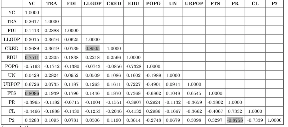
Table 5 includes the correlation matrixes of the selected explanatory variables. According to

correlation between two independent variables is more than 0.75. Result confirms this issue between some variables. Concerning financial development and infrastructure indices, the results strikingly demonstrated the massive differences in both indices. With reference to the financial development index, China, Thailand and Switzerland generally present the best scores given that they are placed on the frontier.

The rest of the selected countries present lower scores: less than 0.5. It is important to note that all countries improved their scores over the period. Scores of the infrastructure index reveal that with the exception of Switzerland, India,

Poland and Togo, the rest of the selected countries are below the frontier. This is due to infrastructural shortcomings across all the components.

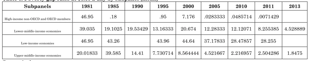
Poverty reduction is an overriding goal and also the most important challenge for all countries. Tables 6 and 7 present the regional average poverty levels. There is clear evidence of a decline in poverty over the year. However, poverty reduction has been quite disparate across groups. In fact, the most pronounced decline was registered in Upper-middle-income economies since the 2000s. Lower-middle-income economies came second. Poverty in Low-income economies is high compared to other groups, albeit declining. Poverty in High-income non-OECD and OECD members is in the low end of the scale. Significant differences exist among countries.

For example, India, Senegal, Chad, Tanzania, Niger, Sierra Leone, Benin and Togo hold the record of the highest poverty rates (Poverty headcount ratio at $3.10 a day >50%) over the last three years. Belarus, Croatia, Czech Republic, Estonia Hungary and Lithuania have relatively lower poverty rates.

Table 6: Poverty gap ratio at $3.10 a day by subpanel (mean)

Subpanels 1981 1985 1990 1995 2000 2005 2010 2011 2013

High-income non-OECD and OECD members 46.95 .18 .95 7.176 .0283333 .0485714 .0071429

Lower-middle-income economies 39.035 19.1025 19.53429 13.16333 20.674 12.28333 12.12071 8.255385 4.528889

Low-income economies 46.95 43.26 43.96 44.64 37.17833 28.47857 28.255

Upper-middle-income economies 20.01833 39.585 14.41 7.730714 8.564444 4.521667 2.216957 2.504286 1.8475

Source: Authors

Table 7: Poverty headcount ratio at $3.10 a day by subpanel (mean)

Subpanels 1981 1985 1990 1995 2000 2005 2010 2011 2013

High-income non-OECD and OECD members 91.54 .39 5 15.444 .095 .1257143 .0514286

Lower-middle-income economies 70.335 48.355 45.81571 35.70778 46.777 33.55733 28.80786 22.52923 12.62444 Low-income economies _91.54 _91.15 _86.44 _85.23667 _74.335 _63.12 _64.4175

Upper-middle-income economies 39.815 58.03 34.69429 18.62571 21.51222 12.0975 7.563913 7.800476 5.2925

Source: Authors.

Results and Discussions

Analysis of the Static Panel Data Estimations

Results from estimating equations (1) and (2) are presented in Tables 8–17. Turning first to the overall sample, the results regarding some economic variables are puzzling. In fact, the impacts of FDI and degree of economic openness on poverty reduction were positive but not significant (Tables 8-9,

R4-R5). In explaining this phenomenon, we can state that the effects of trade and FDI do not accrue automatically and additional policies

are needed to improve their benefits 

2-3-8.In fact, the poverty reduction effects of

(12)

liberalization and FDI inflows are accompanied by poverty reduction if the education system enables skills to match evolving needs of expanding sectors (creation and application of new knowledge and technologies). The connection between trade openness (or FDI) and poverty may hinge on a country's political environment. Key freedoms promote trade and investment: they provide a basis for improving the working environment, broadening social opportunity and helping market access.

Le Goff and Singh 3, formulated others

possible explications. There is too much heterogeneity in the effects of trade reforms on the poor since poor employees in import-competing sectors lose from reforms, whereas poor employees in export-oriented sectors gain. Using a large sample may increase the degrees of freedom but introduce unwanted heterogeneity if factors explaining poverty differ between country groups.

The results also suggest a significant negative correlation between GDP per capita and poverty outcomes. This relationship holds even after controlling for financial market development, education and political variables. This finding reveals that more developed countries have lower levels of poverty.

As expected, the impact on poverty of Private credit by deposit money banks and other financial institutions to GDP ratio is significant and negative for our entire sample. We could deduce that an increase in credit by financial intermediaries to the

private sector may promote private

investments in the productive sectors, which ultimately leads to growing middle-income class and reduces poverty. Contrary to expectations, the ratio liquid liabilities as percent of GDP has a positive sign, but it failed to achieve any conventional level of significance. The result has the same

direction with Jeanneney and Kpodar 54

findings.

Concerning the political variables, our results reveal that there is a positive correlation between civil liberty and poverty reduction (Table 8: R2-R3): Better individual rights

would decrease poverty3_{. When we examine}

3_{The exclusion of political right and country’s political regime}

variables has not changed the sign and significance of the

the role of political right and country’s political regime, the coefficients are generally not significant and positive.

As regards the socio-cultural variables (Tables 8-9: R1-R2-R3), most of them have the expected sign and are significant. The coefficient for education is negative and significant. Therefore, an increase in the level of school enrolment not only decreases headcount but also decreases the intensity of poverty. Unlike population growth and unemployment, the process of urbanization is related to decreasing poverty. The positive effect of infrastructure on poverty reduction

is uncontroversial4_.

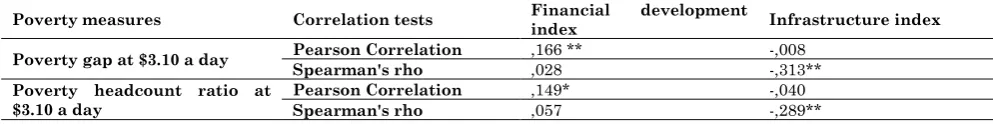
Because the number of observation is insufficient to estimate our equation, we use

scatter plots (not reported here)5_and

correlation analyses (Table 10) to define the relationship between infrastructure and financial development indices and poverty measures. We may say that there is a relationship between financial development and infrastructure indices and poverty measures. According to Spearman's rank-order correlation, there is a weak negative correlation between infrastructure index and poverty measures. The significant Pearson correlation coefficient values confirm that large values of financial development index are associated with large poverty value.

The interactive model generally displays the expected signs of the coefficients (Table 8: R6-R7 and Table 9: R6-R7). It means that the beneficial impact of trade liberalization is larger when the investment in human capital is stronger. Besides, the result suggests that trade is associated with lower levels of poverty when the financial sector is more developed: more access to cheaper credit may allow the poor to benefit more from trade

openness.

When we compare magnitudes of the coefficients to each other (Tables 8 and 9), we note that generally the impact from a 1 unit change in X on poverty gap ratio is greater than the impact from a 1 unit change on Poverty headcount ratio.

To ensure the robustness of the results, the results. We may say that the robustness is achieved for the estimated results.

4_{There is evidence that poverty outcomes vary negatively with}

the level of infrastructure (Arable land and Electric power consumption variables). Results are not reported. For more details, contact authors.

(13)

addition and the removal of explanatory variables were been examined. Results reveal generally that all coefficients maintain their degree of significance and the signs are not changed. We also considered other variables: We found that export growth, size of the public sector, ability to pay, inflation, exchange rate and gross domestic savings do not have a significant impact on any of the

poverty indicators6_.

Moving our focus to the results by subpanels (Tables 11-12-13-14-15-16-17-18). There are considerable regional differences in the

responsiveness of poverty to the

determinants. Lower-middle-income

economies and Upper-middle-income

economies are more affected by poor

environmental and socio-economic

conditions.

Overall, the impact of education and

population growth varies from one group to another. Education seems to be robustly linked to poverty only for Upper-middle-income economies (Tables 17-18: R1-R2-R3). Education is relevant and purposeful: it could

create employment opportunities for

marginalized groups. Low-income economies are typically characterized by low levels of human capital. Education in Upper-middle-income economies is improving rapidly. High-income non-OECD and OECD members are with a very high School enrollment, secondary (% gross) ratio.

Population growth penalizes Lower-middle-income economies: a positive and statistically significant effect (Table 13: R1-R2-R3). The overall population growth does not feed poverty for the other subpanels. The observation of data reveals that population growth rates have declined in Lower-middle-income countries over the past few decades but remain higher than in High-income countries. Demographic projections between 2015 and 2030 suggest that this gap will persist 55.

According to Tables 13, 16, 17 and 18 (R1-R2-R3), unemployment increases poverty in Lower-middle-income economies and Upper-middle-income economies. Statistics show that unemployment is pervasive and vary widely in those nations, reaching as high as

6_{Results are not reported. For more details, contact authors.}

15%, even more than 30% in some countries.

There is also evidence that demonstrates that increase in urban population share causes a decrease in the poverty gap except in the Low-income economies. Unlike population growth, we may say that urban population is a demographic gift. According to the United

Nations 56, the share of the urban

population exceeded the share of people living in the rural areas at the global level.

Unlike Upper-middle-income economies,

Low-income economies suffer relatively from slow urbanization. Generally, in advanced countries, the urbanization induces an increasing share of the labor force in the search for employment opportunities in the non-agricultural industries and services. The development of those sectors may be associated with a rise in household incomes and a significant reduction in poverty. However, in the least developed countries, the negative aspects of urbanization are often observed. Those countries are burdened by a weak agricultural sector (limited employment options, low wages, low productivity, etc) and a weak flourish of non-agricultural sector.

Besides, governments should provide

important services (infrastructure,

transportation, employment, education,…) in order to satisfy the needs of their growing urban populations and to assume the expansion of the non-agricultural sector. Those objectives may be quite critical because the cost of implementing reforms is important and they are unable to devote an important of GDP for infrastructure because low-income levels.

In comparison to the other regions,

Low-income countries suffer from an

infrastructure deficit, with a gap widening

over time. However, the coefficient of

infrastructure has the expected sign and its magnitude is sizeable in the sense that it is larger than the others coefficients (Tables 15-16: R1-R2).

We notice that the coefficients associated with political variables are negative and statistically not significant except for Lower-middle-income economies: Civil rights and

(14)

with Moore and Putzel 57: they found that there is no systematic or deterministic connection between democracy and poverty reduction. Looking at the data, we note that before 1990s, Low-income economies are characterized by a coherent autocracy. Since 1990s, they are characterized by an incoherent regime. High-income non-OECD and OECD members are characterized by a coherent democracy since 1990s.

Lower-middle-income and Upper-middle-income economies have not recorded a major reversal of democratic trend: they are characterized by an incoherent regime. The political scores by income group reveal that low-income economies maintain relatively high scores in terms of political and civil rights. Since 1990s, High-income non-OECD and OECD members have a higher level of political rights and civil liberties. Upper-middle-income economies have weaker institutionalization of political rights and civil liberties than lower-middle income economies.

The results also indicate that GDP per capita is an important instrument for reduction of poverty and the magnitudes of the coefficients are higher for Upper-middle-income economies.

Unlike GDP per capita, the available results for trade openness point toward less than unanimous conclusions. Thus, there is at least some evidence that trade is pro-poor. In fact, trade openness has a significant impact in Low-income economies (Tables 15 and 16: R3-R4).

For the other subpanels, the coefficient of trade is generally positive and not significant. Over the past decade, all countries made trade a key part of their

development strategy. However,

Low-income economies have a small market share: the ratio Exports + Imports)/ GDP annually averaged 56.30 % over the 1981–2013 sample. In contrast, it averaged over 100 % in High-income non-OECD and OECD members (114.59 %). The average ratio for Lower-middle-income economies and Upper-middle-income economies are 76.95 % and 80.57 %, respectively. However, the evidence shows that there is an unequal distribution of the benefits of trade and not all countries are able to fully access the opportunities trade offers. The type of goods and services traded

influences trade-poverty nexus.

Low-income economies have a growing share of

world trade in manufactured goods.

According to the World Bank 58, “Trade

flows among high-income and low-and middle-income economies reveal the changing mix of exports to and imports from developing economies: While food and primary commodities have continued to fall as a share of high-income economies’ imports, manufactures as a share of goods imports from both low- and middle-income economies have grown…………. Yet trade barriers remain high”.

The lack of any clear correlation between FDI and poverty indicators is obvious (Tables 11-12: R1-R2, Tables 13-14-17-18: R4-R5, Tables 15-16: R3-R4). Our result is inconsistent with

the findings of Honohan 59. As mentioned

previously, FDI could influence poverty reduction in the host country through a variety of ways: There are direct and indirect reduction effects that depend on a number of economic characteristics (taxes paid by FDI and how these taxes are spent, productivity of the investments and wages,…).

Besides, FDI flows are characterized by an uneven distribution: At the beginning of the period considered, most of FDI goes to middle and High-income non-OECD and OECD members. The share of FDI net inflows to Low-income economies increased during the last years because of decreasing inflows to

High-income non-OECD and OECD

members.

For Low-income economies (Table 16: R5) and Upper-middle-income economies (Tables 17 and 18: R6), the interactive term TRA*EDU suggests that to have a significant impact on poverty, it is necessary to combine trade liberalization with other policies especially human capital accumulation promotion.

Given the magnitude of the negative sign of the interactive term TRA*CRED, a deep financial market ensures that the overall impact of trade would be negative, as one would ordinarily expect for lower-middle-income economies, Low-lower-middle-income economies and upper-middle-income economies (Tables 13-17: R7 and Table 15: R6).

(15)

(at the 10% level) just for Lower-middle-income economies (Tables 13-14: R5). The coefficient of the ratio of private credit by deposit money banks and other financial institutions to GDP is significant and negative regardless of the subpanel. On average, the highest ratios are found in High-income non-OECD and OECD members (68.60 % from 1981–2013) as opposed to in Low-income economies (24.12 %). The annual average value of private credit across countries is 29.34 %. Averaged over 1981– 2013, the private credit of financial

institutions is less than 25 % of the GDP in lower-middle-income economies and low-income economies (22.47 % of GDP and 13.83 % of GDP, respectively), while exceeding 50 % of GDP in High-income non- OECD and OECD members. It is important to note that a high ratio of private sector credit to GDP is not necessarily a good thing. Since 2008, many countries, such as Switzerland, have

had a major crisis episode 60. On the whole,

there is less clarity, however, on

FDI-financial market depth interaction.

Table 8: Estimation Results-Determinants of Poverty gap at $3.10 a day (2011 PPP) (%): whole sample

Variables R1 R2 R3 R4 R5 R6 R7 R8

C 7.304***

(6.63)

6.56*** (5.83)

6.714*** (4.92)

19.638*** (21.85)

-.499*** ( -5.61)

3.172 (0.62)

8.126*** (4.09)

18.545*** (17.66)

YC -2.137*** _(-21.32) -1.788*** _(-14.61) -1.676*** _(-10.99) -1.778*** _(-15.50) -1.881*** _(-14.29)

TRA .0785 _(0.53) .202 _(1.34) 3.533*** _(2.90) 2.332*** _(5.61)

FDI -.021 _(-0.71) .011 _(0.36) .111 _(0.55) -.115 _(-1.47) .122** _(1.98)

LLGDP .164 _(1.16)

CRED -.499*** _(-5.61) -.287*** _(-3.51) 2.518*** _(4.87)

EDU -.383*

(-1.96)

-.334*** (-1.71)

-.376 (-1.64)

3.212*** (2.65)

POPG .364***

(5.53)

.330*** (4.86)

.466*** (6.27)

UN .475*** _(4.87) .463*** _(4.77) .492*** _(4.81)

URPOP -1.197*** _{(-3.93 )} -1.129*** _(-3.77) -1.158*** _(-3.32)

FTS -.252*** _(-2.62) -.264*** _(-2.73) -.240** _(-2.05)

PR -.103 _(-0.78)

CL .387** _(2.13) .334** _(1.98)

P2 .006

(0.06)

.074 (0.67)

TRA*EDU -.825***

(-2.81)

FDI*EDU -.027 _(-0.54)

TRA*CRED -.676*** _(-5.57)

FDI*CRED .039 _(1.54)

FDI*P2 -.108* _(-1.94)

R-SQ 0.5038 0.5178 0.5602 0.5153 0.4914 0.5764 0.5038 0.5116

N. OBS 437 435 359 778 649 485 662 522

(16)

Table 9: Estimation Results-Determinants of Poverty headcount ratio at $3.10 a day (2011 PPP) (%): whole sample

Variables R1 R2 R3 R4 R5 R6 R7 R8 R9

C 7.485*** _(7.68) 6.528*** _(6.66) 6.961*** _(5.78) 17.976*** _(22.50) 15.459*** _(17.64) 1.663 _(0.37) 6.009*** _(3.47) 17.600*** _(12.50) 16.961*** _(18.49)

YC

-1.831*** (-20.48)

-1.457*** (-13.29)

-1.467*** (-10.69)

-1.461*** (-14.29)

-1.520*** (-14.64)

-1.579*** (-13.74)

TRA .106 _(0.81) .186 _(1.41) 3.524*** _(3.27) 2.439*** _(6.80) -.232*** _(-0.87)

FDI -.011 _(-0.41) .021 _(0.82) .019 _(0.11) -.145** _(-2.16) .128** _(2.50)

LLGDP .103

(0.83)

CRED -.452*** _(-5.82) -.293*** _(-4.05) 2.697*** _(6.06) -.280*** _(-5.59) -.264*** _(-5.23)

EDU -.232 _(-1.38) -.167 _(-1.00) -.180 _(-0.90) 3.551*** _(3.33)

POPG .318*** _(5.73) .281*** _(4.91) .363*** _(5.68)

UN .399*** _(4.73) .381*** _(4.58) .388*** _(4.35)

URPOP -1.121*** _(-4.07)

-1.034*** (-3.89)

-1.164*** (-3.69)

FTS -.169** _(-2.05) -.184** _(-2.24) -.173* _(-1.70)

PR -.089 _(-0.81)

CL .458*** _(3.00) .426*** _(2.94) -1.379* _(-1.65)

P2 .016 _(0.17) .048 _(0.52)

TRA*EDU -.855***

(-3.31)

FDI*EDU .002 _(0.06)

TRA*CRED -.716*** _(-6.86)

FDI*CRED 6.009*** _(3.47)

TRA*CL .330* _(1.76)

FDI*P2 -.089* _(-1.92)

R-SQ 0.4819 0.5205 0.5389 0.5128 0.4798 0.5667 0.4960 0.5105 0.5078

N. OBS 439 437 352 782 652 489 666 676 525

***(**/*) denotes statistically significant at the 1%(5%/10%) level. Robust standard errors in brackets. Variables have been log-transformed. A static random effects model is estimated.

Table 10: Correlation

Poverty measures Correlation tests Financial _index development Infrastructure index

Poverty gap at $3.10 a day Pearson Correlation _{Spearman's rho} ,166 ** _,028 -,008 _-,313** Poverty headcount ratio at

$3.10 a day Pearson Correlation Spearman's rho ,149* ,057 -,040 -,289**

(17)

Table 11: Estimation Results-Determinants of Poverty gap at $3.10 a day (2011 PPP) (%): High-income non-OECD and OECD members

Variables R1 R2 R3

C 34.240*** _(5.81) 35.032*** _(4.11) 71.338*** _(3.92)

YC -4.205*** _(-6.44) -4.336*** _(-5.09) -3.275** _(-3.66

TRA 1.005 _(1.45) .162 _(0.17) -11.109** _(-2.53)

FDI .156 _(0.78) .155 _{( 0.54)} 4.268** _(2.28)

LLGDP .279

( 0.19)

CRED .860 _(0.97) -11.327** _(-1.99)

EDU TRA*EDU FDI*EDU

TRA*CRED 3.026**

(2.38)

FDI*CRED -1.139** _(-2.25)

R-SQ 0.6183 0.7323 0.6331

N. OBS 58 40 51

Table 12: Estimation Results—Determinants of Poverty headcount ratio at $3.10 a day (2011 PPP) (%): High-income non-OECD and OECD members

Variables R1 R2 R3

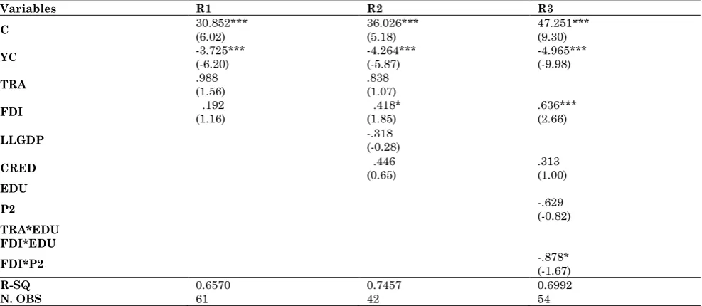
C 30.852*** _(6.02) 36.026*** _(5.18) 47.251*** _(9.30)

YC -3.725*** _(-6.20) -4.264*** _(-5.87) -4.965*** _(-9.98)

TRA .988 _(1.56) .838 _(1.07)

FDI .192 _(1.16) .418* _(1.85) .636*** _(2.66)

LLGDP -.318

(-0.28)

CRED .446 _(0.65) .313 _(1.00)

EDU

P2 -.629 _(-0.82)

TRA*EDU FDI*EDU

FDI*P2 -.878* _(-1.67)

R-SQ 0.6570 0.7457 0.6992

N. OBS 61 42 54

(18)

Table 13: Estimation Results-Determinants of Poverty gap at $3.10 a day (2011 PPP) (%): Lower-middle-income economies

C 6.702*** _(4.69) 5.773*** _(3.75) 6.419*** _(3.24) 19.452*** _(11.81) 15.190*** _(8.19) 10.522 _(1.06) .607 _(-0.24) 8.390 _(1.42) 27.201*** _(6.87)

YC -2.191*** _(-11.46) -1.686*** _(-7.15) -1.681*** _(-5.47) -1.639*** _(-8.74) -1.941*** _(-7.83) -1.756*** _(-8.56)

TRA .298 _(1.31) .439** _(1.99) 1.819 _(0.78) 4.188** _(8.87) 2.660** _(2.07) -2.277*** _(-2.80)

FDI -.090 _(-1.64) -.002 _(-0.06) .3757 _(0.54) -.277** _(-2.40

LLGDP .363* _(1.65)

CRED -.629***

(-4.93)

-.453*** (-3.38)

4.884*** (7.67)

-.314*** (-4.44)

-.252*** (-4.11)

EDU -.290 _(-1.34) -.303 _(-1.41) -.621** _(-2.35) 1.381 _(0.56)

POPG .263** _(2.13) .328*** _(2.58) .261* _(1.81)

UN .286** _(2.55) .302*** _(2.63) .554*** _(3.59)

URPOP -.915*** _{( -2.63)} -.856** _(-2.40) -.761 _(-1.58)

FTS -.086 _{(-0.90 )} -.0251 _(-0.25) -.065 _(-0.48)

PR -.243* _(-1.66)

CL .708**

(2.28)

.100 (0.29)

-9.116*** (-3.47)

P2 .208 _(0.70) 4.595* _(1.77)

TRA*EDU -.352 _(-0.61)

FDI*EDU -.085 _(-0.49)

TRA*CRED -1.237*** _(-8.40)

FDI*CRED .095** _(2.47)

TRA*P2 -1.112* _(-1.74)

TRA*CL 2.198***

(3.70)

R-SQ 0.4139 0.4448 0.4344 0.3631 0.2894 0.2656 0.3218 0.3323 0.2741

N. OBS 129 129 99 269 228 157 230 188 236

(19)

Table 14: Estimation Results-Determinants of Poverty headcount ratio at $3.10 a day (2011 PPP) (%): Lower-middle-income economies

C 6.763*** _(6.61) 6.059*** _(5.59) 6.997*** _(4.87) 16.672*** _(12.17) 12.699*** _(8.73) 10.330 _(1.30) 9.115* _(1.91) 13.605*** _(9.01) 22.716*** _(7.19)

YC -1.672*** _(-10.57) -1.185*** _(-6.45) -1.170*** _(-4.83) -1.454*** _(-7.41) -1.178*** _(-6.86) -1.267*** _(-7.85)

TRA .179 _(0.95) .273 _(1.57) .989 _(0.53) 1.749* _(1.67) -1.967*** _(-3.04)

FDI -.080* _(-1.72) -.016 _(-0.40) .505 _(0.89) -.304* _(-1.86)

LLGDP .340*

(1.98)

CRED -.566*** _(-5.58) -.408*** _(-3.82) -.265*** _(-4.63) -.210*** _(-4.06) -.215*** _(-4.40)

EDU -.224 _(-1.46) -.232 _(-1.54) -.400** _(-2.12) .809 _(0.41)

POPG .133 _(1.51) .182** _(2.04) .107 _(1.03)

UN .259*** _(3.23) .267*** _(3.30) .463*** _(4.23)

URPOP .720*** _(-2.87) -.680*** _(-2.69) -.775** _(-2.14)

FTS .058 _(-0.85) -.010 _(-0.15) -.074 _(-0.77)

PR -.228**

(-2.24)

CL .590*** _(2.71) .014 _(0.06) -7.407*** _(-3.55)

P2 .165 _(0.79) 3.123 _(1.49) .255 _(1.05)

TRA*EDU -.194 _(-0.42)

FDI*EDU -.121 _(-0.87)

TRA*P2 -.763 _(-1.48)

FDI*CL .217* _(1.72)

TRA*CL 1.804***

(3.82)

R-SQ 0.4799 0.5328 0.4717 0.3677 0.3143 0.2967 0.3468 0.3837 0.2891

N. OBS 129 129 99 269 228 157 188 230 236

(20)

Table 15: Estimation Results-Determinants of Poverty gap at $3.10 a day (2011 PPP) (%): Low-income economies

Variables R1 R2 R3 R4 R5 R6 R7

C 3.689*** _(5.08) 4.839*** _(5.31) 12.406*** _(13.52) 9.670*** _(9.98) 5.540** _(2.36) 6.488*** _(4.26) 9.254*** _(10.15)

YC -.968***

(-7.21)

-.627*** (-4.38)

-.474*** (-2.95)

-.665*** (-4.74)

-.644*** (-4.98)

TRA -.475*** _(-3.44) -.295** _(-2.50) .592 _(1.15) .585 _(1.64)

FDI -.0087 _(-0.35) -.001 _(-0.08) .090 _(1.39) -.002 _(-0.06) -.018 _(-0.12)

LLGDP .066 _{( 0.44)}

CRED -.247* _(-2.15) -.120* _(-1.70) 1.246** _(2.20) -.249*** _(-3.68)

EDU -.247* _{(-1.65 )} -.220 _(-1.47) .766 _(1.31)

POPG -.181 _(-1.61) .192* _(-1.70)

UN .102

(1.16)

.141 (1.52)

URPOP .152 _(0.82) -.014 _(-0.07)

FTS -.348*** _(-3.58) -.328*** _(-3.34)

PR -.079 _(-0.26)

CL -.466 _(-1.05) -.329** _(-2.05)

TRA*EDU -.232 _(-1.61)

FDI*EDU -.041* _(-1.84)

TRA*CRED -.359**

(-2.58)

FDI*CRED .0006 _(0.03)

FDI*CL .001 _(0.02)

R-SQ 0.5972 0.6260 0.6929 0.6787 0.7892 0.6807 0.5962

N. OBS 61 61 85 72 47 72 76

Table 16: Estimation Results-Determinants of Poverty headcount ratio at $3.10 a day (2011 PPP) (%): Low-income economies

Variables R1 R2 R3 R4 R5 R6

C 4.341*** _(9.57) 4.926*** _(8.53) 9.012*** _(17.35) 7.274*** _(12.96) 4.772*** _(3.39) 7.280*** _(14.50)

YC -.496*** _(-6.36) -.292*** _(-3.52) -.231** _(-2.42) -.329*** _(-4.63)

TRA -.290*** _(-3.58) -.159** _(-2.25) .407 _(1.32)

FDI -.003

(-0.24)

-.003 (-0.28)

.052 (1.34)

-.002 (-0.03)

LLGDP .011

(0.13)

CRED -.109 _(-1.60) -.072* _(-1.71) -.119*** _(-3.12)

EDU -.089 _(-0.95) -.079 _(-0.84) .559 _(1.58)

POPG -.080 _(-1.14) -.089 _(-1.26)

UN .038 _(0.70) .053 _(0.91)

URPOP .048 _(0.42) -.033 _(-0.27)

FTS -.201***

(-3.30)

-.187*** (-3.02)

PR -.093

(-0.48)

CL -.169 _(-0.60) -.233** _(-2.53)

TRA*EDU -.154* _(-1.77)

FDI*EDU -.025* _(-1.84)

FDI*CL -.006 _(-0.11)

R-SQ 0.5261 0.5489 0.6341 0.6161 0.7376 0.5856

(21)

Table 17: Estimation Results-Determinants of Poverty gap at $3.10 a day (2011 PPP) (%): Upper-middle-income economies

C 15.475*** _(7.83) 15.232*** _(7.64) 13.575*** _(6.21) 24.558*** _(14.43) 20.868*** _(11.06) -4.425 _(-0.35) 2.512*** _(2.98) 25.019 _(9.21) 23.885*** _(11.47)

YC -2.69***

(-15.04)

-2.120*** (-9.18)

-1.818*** ( -6.69)

-1.990*** (-8.57)

-2.255 (-9.22)

-2.396*** (-9.66)

TRA .257

(1.10)

.272 (1.15)

6.125** (2.06)

2.036** (2.48)