JEEECCS, Volume 1, Issue 2, pages 37-41, 2015
Neural Networks Versus Classic Mathematical
Models to Estimate Gasoline Blending
Properties
Bogdan Doicin
Electric and Mechanic Engineering Faculty Oil-Gas University
Ploiești, Romania [email protected]
Cristian Pătrășcioiu
Electric and Mechanic Engineering Faculty Oil-Gas University
Ploiești, Romania [email protected]
Abstract – Nowadays, gasoline must comply with a number of quality standards, whose purpose is the pollution reduction due to the produces that result from gasoline burning. These quality standards have a connection with the gasoline properties. The determination of gasoline properties is being made according to the standards. The standard methods’ drawbacks are related to determination duration, the fact that some methods are destructive and the obtained results are useful as long as the components’ properties are constant. To offset these drawbacks, the possibility of gasoline properties estimation became attractive.
In this paper, a comparative study between two estimation methods for gasoline properties is presented. The first method is based on a mathematical model which has 8 equations, model that can be found in the literature. The second method uses artificial neural networks for estimation. To be able to compare these methods, 60 blendings based on 60 different blending recipes were prepared. These blendings’ components are: FCC gasoline, catalytic reforming (CR) gasoline, iC5 fraction and bioethanol. The obtained results from this comparative study can be used to determine which of these two methods offers the most precise estimation in a particular case.
Keywords – comparative study, neural networks, mathematical models, gasoline properties estimation
I. INTRODUCTION
The gasoline is a fuel whose demand constantly increased in the last decades, with the increase of the number of vehicles. Nowadays, the legislative framework regarding gasoline state that its properties must be within a scope, to reduce the pollution caused by gasoline burning. Among the most important laws is the EN 228 standard [1].
Nowadays, gasoline can be obtained by blending of its components, process called formulation. The utilized components and their properties form a
blending recipe. The blending recipe must be made so
as the final blending respects today’s standards regarding gasoline characteristics.
The gasoline properties are experimentally determined according to the standards. The drawbacks of these determination methods refer to the time duration, the fact that some methods are destructive, and that the obtained results are useful as long as the components’ properties are constant. To offset these drawbacks, more and more attractive became the possibility of estimating the gasoline properties. Among the estimation methods are the methods based on mathematical equations and those based on neural networks.
II. BLENDING PROPERTIES’ ESTIMATION METHODS Gasoline blending mathematical modelling was the object of intense research in the last decades, periods in which many mathematical methods where developed. Among these methods are the method based on linear blending models and the method based on neural networks.
The purpose of these methods are to estimate the gasoline blending properties for different blending recipes.
A. Linear blending models
This research started from the mathematical model developed by Bărbatu, based on own experimental data [2]. Starting from data presented in the literature, a higher complexity model, based on the following equations, was tested [3]:
Blending density [g/cm3]:
xix/di
Research Octane Number (RON) [octane units]:
COR=(CORi*xi)
Motor Octane Number (MON) [octane units]:
COM=(COMi*xi)
Ar=(Ari*xi)
Olefin hydrocarbon content [% vol.]:
Ol=(Oli*xi)
Oxygenated compounds content [% vol.]:
Ox=(Oxi*xi)
Vapor pressure [kPa]:
Pv=(Pvi*xi)
Benzene content [% vol.]:
Bz=(Bzi*xi)
The notations from the equations (1)-(8) have the following significance:
– blending density [kg/cm3];
di – the i-th component density of the blending [kg/cm3];
xi – the i-th component proportion in the blending [% vol.];
COR – blending MON;
CORi – the RON of the i-th component of the blending;
COM – blending MON;
COMi – the MON of the i-th component of the blending;
Ar – the blending aromatic hydrocarbon content [% vol.];
Ari – the aromatic hydrocarbon content of the
i-th component of the blending [% vol.];
Ol – the blending olefin hydrocarbon content [% vol.];
Oli – the olefin hydrocarbon content of the i-th component of the blending [% vol.];
Ox – the blending oxygen content [% vol.];
Oxi – the oxygen content of the i-th component of the blending [% vol.];
Pv – the blending vapor pressure [kPa];
Pvi – the vapor pressure of the i-th component of the blending [kPa];
Bz – the blending benzene content [%vol.];
Bzi – the benzene content of the i-th component of the blending [% vol.].
B. Estimation methods based on neural networks
The second category of gasoline properties’ estimation methods is based on using neural networks. Generally, an artificial neural network (ANN) is an algorithm that simulates the human brain functioning.
The ANN can be utilized to estimate the blending properties when the properties of the blending components and the properties which need to be estimated in the resulting blend are known. Applying the ANN method has two steps.
The first step is represented by determining the input and the output data, between the two kinds of data a causal link must be existing. To correctly implement this step, in this paper, the input data are the components’ properties and the output data are the blending properties.
The second step is training the ANN. From a programming point of view, ANN training is a process in which some ANN internal parameters are adjusted so as, when the ANN will be used, the estimations obtained by the user are as close as possible to the data used for training.
To be able to use an ANN, using some sets of experimental data is required. The experimental data are organized into a database, called training
database. This database has two main characteristics:
the number of records (data volume) and the data correlation degree. Between these two characteristics, the data correlation degree is more important.
While training the ANN, the data from the training database are split into three categories: training data,
validation data and testing data. The ratio in which the
data is split into these categories may vary, but, usually, 70% of the data from the training database are training data, while the other 30% are split equally between validation and testing data.
After the end of the training process, there are more methods to check the ANN training efficiency. Among them are the error histogram and the data
regression analysis. The more efficient the ANN
training was, the more precise the ANN is, relating to the data from the training database. If the training efficiency is unsatisfactory, there are two ways to try to improve it:
Using another training dataset (or adding new data to the existing ones), followed by an ANN training;
ANN re-training, using the same training database. The reason is that the data distribution by the three categories is random and it’s possible that a re-training of the ANN will be more efficient because of another data distribution.
The basic component of an ANN is a functional unit called neuron. The more neurons the neural network has, the more accurate are the network’s estimations, as long as overtraining does not occur.
A neural network has three layers:
The hidden layer. Its purpose is to process the input data received from the input layer and to send the results to the output layer;
The output layer. Its purpose is to display the obtained results. The number of the neurons from the output layer is equal to the number of the output data, because one neuron can
store only one output data [4].
In figure 1, an example of a structure of a neural network which is used to estimate the gasoline blending properties is presented. This ANN has one neuron in the input layer, 10 neurons in the hidden layer and one neuron in the output layer. The number of 10 neurons was chosen because it was the lower number of neurons for which the data regression analysis showed a correlation coefficient over 0.95 for all the categories in which the training data were divided. Increasing the number of neurons didn’t lead to significant improvements and/or lead to over-training.
During ANN training, the Levenberg-Marquardt algorithm was used. This training algorithm, was chosen because it is designed for training databases of low dimensions. The desired error was reached in the 19th epoch.
In this paper, the input data used by the ANN are the proportions in which are blend the gasoline components, proportions expressed in % vol. The output data are the blending density [g/cm3], MON and RON [octane numbers], benzene content [% vol.], vapor pressure [kPa], olefin hydrocarbon content [% vol.], aromatic hydrocarbon content [% vol.] and oxygen content [% vol.].
III. APPLYING THE ESTIMATION METHODS OF GASOLINE BLENDING PROPERTIES
A. Gasoline blending
The blending properties were studied and presented in many papers, some of them being [2, 5, 6, 7, 8, 9]. Experimental gasoline blendings using four components: FCC gasoline, catalytically reforming (CR) gasoline, isopentane fraction (iC5) and bioethanol, were generated. Each component was experimentally characterized, being determined the following properties: RON, MON, benzene content, olefin content, aromatic hydrocarbons content, oxygen content, vapor pressure and density [5].
Using the four components, 60 blendings were experimentally obtained, each blending having a different blending recipe. Each of these blendings was experimentally characterized, being determined the
aforementioned properties. Thus, a database was created, which contains [5]:
The physical properties of each component used in gasoline blending.
Components’ blending recipe.
The physical properties of the experimentally obtained gasoline blendings.
B. Results using the linear blending models
The model that uses the linear blending model required using the equations (1) - (8), which helped to compute the properties of the gasoline blendings according to the experimental blending recipes. The estimation error of the model in relation with the experimental data for each property is calculated with the following equation:
e=((|yj(exp)-yj(model)|))/(yj(exp)) [%]
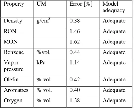
The obtained results are presented in table 1. Small values of the estimation error prove the blending model adequacy.
Table 1 Model adequacy, based on the obtained experimental data
Property UM Error [%] Model
adequacy
Density g/cm3 0.38 Adequate
RON 1.46 Adequate
MON 1.62 Adequate
Benzene %vol. 0.44 Adequate
Vapor pressure
kPa 1.14 Adequate
Olefin % vol. 0.42 Adequate
Aromatics % vol. 0.40 Adequate
Oxygen % vol. 1.38 Adequate
C. Results using the neural network model
To create, train and use the ANN, MATLAB R2012b software was used, respectively the application Neural Network Toolbox.
ANN creation and training were made according to the procedure described in the MATLAB help program. Due to the small number of the used data, the default parameters for neural network creation and training were used. The neural network has 10 neurons in the hidden layer.
Due to the random factor in distributing the data from the training database on each of the three data types, three estimations of the gasoline blending properties were made. Between the estimation, the neural network was trained using each time the same training database. The obtained results are presented in table 2. The results analysis shows similar results between the three ANN estimations, their averages being close to the experimentally determined values.
The adequacy of the blending model based on the neural network was computed similarly to the model based on linear mathematical equations. The results are presented in table 3.
Table 2 Blending properties estimation using the neural network
Property Obtained values
Ave
ra
ge
o
f
es
ti
mate
d
va
lues
E
xpe
ri
menta
ll
y
E
sti
ma
ti
on
1
E
sti
ma
ti
on
2
E
sti
ma
ti
on
3
Density 0.750 0.752 0.746 0.776 0.758
RON 95.9 95.8 96.1 95.8 95.9
MON 85.1 85.2 85.1 85 85.1
Benzene 0.61 0.562 0.628 0.581 0.59 Vapor
pressure
65 65.1 65.6 65.2 65.3
Olefin 5.96 5.8 6.02 6.24 6.02
Aromatics 34.88 35.04 34.87 35.2 35.04
Oxygen 0 0.001 0.002 0 0.001
The analysis of the results presented in table 6 shows that the model based on neural networks estimates the blending properties with errors between 0.02% and 0.46% for octane number, vapor pressure and aromatic hydrocarbon content. For the other properties, the estimation error is too large to consider this blending model to be adequate. In this case, there are two solutions to reduce the estimation errors: ANN re-training, using the same database and neural network re-training using a larger training database. Between these two solutions, preferable is the latter, to reduce the impact of the random factor on the obtained results.
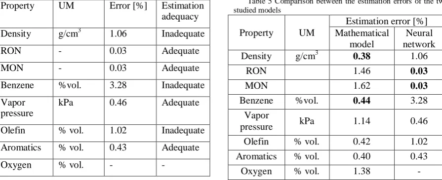
Table 3 Adequacy of the blending model based on neural networks
Property UM Error [%] Estimation adequacy
Density g/cm3 1.06 Inadequate
RON - 0.03 Adequate
MON - 0.03 Adequate
Benzene %vol. 3.28 Inadequate
Vapor pressure
kPa 0.46 Adequate
Olefin % vol. 1.02 Inadequate
Aromatics % vol. 0.43 Adequate
Oxygen % vol. - -
D. Comparision between the estimation methods of
blending gasoline
Table 4 presents, comparatively, the estimations of the gasoline blending properties calculated with the two estimation methods. The results analysis shows a rather even distribution between the good and very good results obtained by the two methods. However, the results presented in table 4 are average results, for the method based on neural networks, not the results obtained directly by properties calculations.
Table 4 Estimations offered by the two studied mathematical models
Property
UM
C
las
sic
al
model Ne
ur
al
ne
twor
k
E
xpe
ri
menta
l
va
lue
Density g/cm3 0.749 0.758 0.750
RON - 94.86 95.90 95.90
MON - 84.20 85.10 85.10
Benzene %vol 0.61 0.59 0.61
Vapor
pressure kPa
64.02 65.3 65
Olefin %
vol
5.64 6.02 5.96
Aromatics % vol
34.88 35.04 34.88
Oxygen %
vol
0 0.001 0
A suggestive comparison of the two methods is obtained if it is taken into account the estimation errors of the blending properties, presented in table 5. From table 5 it can be observed that for the octane numbers and vapor pressure, the estimation error is larger for the classical model, while for the other properties, the model based on neural networks has a larger error.
Table 5 Comparison between the estimation errors of the two studied models
Property UM
Estimation error [%] Mathematical
model
Neural network
Density g/cm3 0.38 1.06
RON 1.46 0.03
MON 1.62 0.03
Benzene %vol. 0.44 3.28
Vapor
pressure kPa 1.14 0.46
Olefin % vol. 0.42 1.02
Aromatics % vol. 0.40 0.43
IV. CONCLUSIONS
In this paper, the estimation performances of two mathematical models to estimate the gasoline blending models: a mathematical model based on equations (1)-(8), presented in the literature and a model based on neural networks was compared.
To compare the two models, 60 blendings were prepared, each blending having a distinct blending recipe, blending which had the following components: FCC gasoline, CR gasoline, isopentane fraction (iC5) and bioethanol.
The mathematical model based on the equations had, relatively to the experimental data, estimation errors between 0.38% and 1.62%. Because of this reason, the conclusion that the mathematical model based on equations is adequate and can be successfully used to estimate the properties taken into account of the gasoline blending can be drawn.
The mathematical model based on neural networks showed, relative to the experimental data, estimation errors between 0.03% and 3.28%. Because of this reason, the mathematical model is inadequate for the estimation of certain of the properties which were taken into account for the gasoline blending (blending density, benzene and olefin hydrocarbon content). The estimation errors for the properties in which the model is inadequate have, as a cause, the low number of experimental data had at the time when the experiments occurred.
Finally, the estimating precisions for the two methods were compared. The estimating precisions are
presented in table 5. According to that table, for the octane numbers and the vapor pressure the estimation error is larger for the classical mathematical model, while for the other properties the neural network model has larger estimation errors.
[1] EN 228 standard, available at http://consiliari.pl/gasoline_en_228/ . Access date: 13 november 2015
[2] B. Doicin, ”Optimizarea Rețetelor de Amestec Pentru Reformularea Combustibililor Ecologici de Tip Benzine” (Teză de doctorat), pag. 48, 2014.
[3] C. Pătrășcioiu, B. Doicin, ”Property Estimation of Commercial Ecological Gasoline”, Chemical Engineering Transactions, vol. 43, pp. 247-252, 2015;
[4] B. Doicin, ”Optimizarea Rețetelor de Amestec Pentru Reformularea Combustibililor Ecologici de Tip Benzine” (Teză de doctorat), pag. 54, 2014;
[5] B. Doicin, C. Pătrășcioiu, C. G. Amza, I. Onuțu, ”Mathematical Model for Studying the Variation of Gasoline-Bioethanol Blend Properties”, Revista de Chimie, nr. 4, pp. 523-528, 2015.
[6] M. Krigina, M. Gyngazova, E. Ivanchina., ”Mathematical Modeling of High-Octane Gasoline Blending, Strategic Technology Conference, Tomsk, 2012.
[7] W. Yu, A. Morales, ”Gasoline Blending System Modeling via Static and Dynamic Neural Networks”, International Journal of Modeling and Simulation, vol. 24, pp. 151-160, 2004. [8] B. Doicin, I. Onuțu, ”Octane Number Estimation Using
Neural Networks”, Revista de Chimie, nr. 5, pp. 599-602, 2014