BIOMECHANICAL MODELING OF CANINE RETRACTION
Matthew Evans Larson, DDS
A thesis submitted to the faculty of the University of North Carolina at Chapel Hill in partial fulfillment of the requirements for the degree of Master of Science in the School of Dentistry (Orthodontics).
Chapel Hill 2012
©2012
ABSTRACT
MATTHEW EVANS LARSON: Biomechanical Modeling of Canine Retraction (Under the direction of Dr. Ching-Chang Ko)
ACKNOWLEDGEMENTS
I would like to thank the following for their contribution, support and dedication:
Dr. Ching-Chang Ko, for his knowledge and mentorship. His constant support made this project successful.
Dr. Tung Nguyen, for providing a vision for moving forward and completing this project, and his assistance with the manuscript.
Dr. Garland Hershey, for his knowledge of the orthodontic literature and advice on the manuscript.
Dr. Kazuo Hayashi, for initial placement of the virtual orthodontic appliances and for use of his clinical data.
Dr. Emile Rossouw, for his assistance with the manuscript and keeping the information accessible to orthodontists.
Dr. Chris Canales, for his knowledge of the Solidworks software. Katie, for her love and support.
My co-residents, for all the good memories.
TABLE OF CONTENTS
LIST OF TABLES... ... vii
LIST OF FIGURES... .viii
LIST OF ABBREVIATIONS... ... xi
I. INTRODUCTION ... 1
i. Overview ... 1
ii. Developments in the biology of orthodontic tooth movement... 2
iii. Properties of the periodontal ligament (PDL) ... 4 16 iv. Influence of force magnitude and duration on tooth movement ... 5 18 v. Current mechanical prediction of orthodontic loading and its limitations ... 6
vi. Finite element analysis ... 7
vii. Well-controlled clinical data on canine retraction ... 13
viii. Hypothesis ... 16
II. MATERIALS AND METHODS ... 18
i. Creation of a complete maxillary biomechanical model... 18
ii. Isolation of a two-tooth substructural model ... 27
iii. Effects of model size, mesh density, PDL properties, and accurate orthodontic appliances ... 29
iv. Comparison of FEA results with clinical data ... 30
III. RESULTS ... 31
ii. Specific Aim 2: Isolation of a two-tooth substructural model ... 34 iii. Specific Aim 3: Effects of model size, mesh density,
PDL properties, and accurate orthodontic appliances ... 34
iv. Specific Aim 4: Comparison of FEA results with clinical data ... 40 16 IV. DISCUSSION ... 42
i. Comparison of results to previous literature ... 42 ii. FEA versus laboratory testing ... 43
iii. Current limitations and further improvements ... 46 18 V. CONCLUSIONS ... 50
APPENDIX 1: Geomagic ... 51 APPENDIX 2: Solidworks 2010 ... 71
LIST OF TABLES
Table 1. Summary of the adaptive response of bone under applied load ... 3
Table 2. Summary of guidelines for force levels during orthodontic treatment ... 6 23 Table 3. XYZ clinical data from Hayashi et al ... 15
Table 4. FHA clinical data from Hayashi et al... 16
Table 5. Techniques used to ensure ideal connectivity ... 23
Table 6. Mesh sizing for the half maxilla model ... 24 23 Table 7. Material properties used for the model (except PDL)... 25
Table 8. Various materials properties tested for the PDL ... 30
Table 9. Summary table of models tested with solution times ... 35
Table 10. Comparison of a coarse mesh with fine mesh (displacement) ... 37 23 Table 11. Comparison of a coarse mesh with fine mesh (stresss and strain) ... 37
Table 12. Comparison of the full model to the substructural model (displacement) ... 38
Table 13. Comparison of the full model to the substructural model (stress and strain) ... 38
LIST OF FIGURES
Figure 1. Summary of clinical data on tooth movement with applied force ... 6 26
Figure 2. Different values for the PDL elastic modulus used by Cattaneo et al ... 9
Figure 3. Clinical setup in canine retraction study by Hayashi et al ... 13
Figure 4. Diagrams of the XYZ and FHA systems used by Hayashi et al ... 15
Figure 5. Problematic geometry fixed in Geomagic ... 20
Figure 6. NURB surfacing in Geomagic ... 21
Figure 7. Final half maxilla model ... 23
Figure 8. Final mesh for the half maxilla model ... 24
Figure 9. Boundary conditions for the half maxilla model ... 26
Figure 10. Displacement probe locations for calculating tooth movement ... 27
Figure 11. Boundary conditions for the substructural model ... 28
Figure 12. Final fine mesh used for the substructural model ... 29
Figure 13. Representative displacement color map for solved complete model... 32
Figure 14. Representative Von-Mises (equivalent) strain for the complete model ... 33
Figure 15. Von-Mises, maximum, and minimum elastic strain in canine PDL ... 33
Figure 16. Substructural model with fine mesh size ... 34
Figure 17. Close-up view of maxillary canine showing no engagement with wire ... 36
Figure 18. Resultant force/moment in the PDL during canine retraction – no wire ... 39
Figure 19. Resultant force in the PDL during canine retraction, 0.5N and 1N – wire... 40
Figure 20. Resultant moment in the PDL during canine retraction,0.5 N and 1N – wire ... 40
Figure 21. Laboratory model used by Badawi et al ... 45
Figure 23. Polygon model of lateral incisor dentin after importing into Geomagic ... 52
Figure 24. Boundary removal in Geomagic ... 52
Figure 25. Separation of interior and exterior surfaces in Geomagic ... 53
Figure 26. Filling holes and gaps in Geomagic... 54
Figure 27. “Mesh doctor” tool in Geomagic ... 55
Figure 28. Defeaturing in Geomagic ... 55
Figure 29. Ideal mesh doctor output in Geomagic ... 56
Figure 30. “Refine polygons “tool in Geomagic ... 57
Figure 31. “Enhance mesh for surfacing” tool in Geomagic ... 58
Figure 32. Moving an object to “Exact Surfacing” in Geomagic ... 59
Figure 33. Autosurfacing in Geomagic ... 60
Figure 34. Contour lines for left lateral incisor dentin in Geomagic ... 62
Figure 35. Summary of surfacing steps and corresponding menus in Geomagic ... 63
Figure 36. “Shuffle patches” menu in Geomagic... 64
Figure 37. Potential errors during surfacing in Geomagic ... 64
Figure 38. Issues with “merge faces” using a non-grid layout in Geomagic ... 65
Figure 39. “Shuffle patches” to create a grid layout in Geomagic... 65
Figure 40. Ideal grid layout and final surface in Geomagic ... 66
Figure 41. Deviation analysis between initial and final surface in Geomagic ... 66
Figure 42. Overall appearance of final surfaces for a tooth in Geomagic ... 68
Figure 43. Individual appearances of final surfaces for a tooth in Geomagic ... 69
Figure 44. Manipulation of the CEJ boundary in Geomagic ... 70
Figure 46. Final Solidworks part file with cut enamel, dentin, and pulp ... 72
Figure 47. “Surface offset” command in Solidworks ... 73
Figure 48. “Surface-fill” and “Surface-knit” commands in Solidworks ... 74
Figure 49. Final half maxilla Solidworks model ... 75
Figure 50. Correct options for saving as an IGES file from Solidworks ... 76
Figure 51. Main screen of ANSYS WorkBench ... 78
Figure 52. Importing previously saved engineering data in ANSYS... 79
Figure 53. Selecting import options in ANSYS DesignModeler ... 81
Figure 54. “Form new part” tool for creation of multibody parts ... 81
Figure 55. Assignment of material properties in Mechanical ... 82
Figure 56. Option to display by material properties in Mechanical ... 83
Figure 57. Manipulation of contact condition in Mechanical ... 84
Figure 58. Contact tool option in Mechanical, allowing calculation of initial contacts ... 85
Figure 59. Output folder for Mechanical, showing typical files to examine errors ... 87
Figure 60. Mesh menu in Mechanical, showing options for altering mesh size ... 88
Figure 61. Static structural menu in Mechanical, showing options for loading conditions .. 89
LIST OF ABBREVIATIONS 2D – Two-dimensional
3D – Three-dimensional
CAD – Computer Aided Design
CAM – Computer Aided Manufacturing
ε – Strain, change in length over initial length (technically engineering strain)
E – Elastic Modulus, Youngs Modulus FE – Finite Element
FEA – Finite Element Analysis FEM – Finite Element Modeling
FJORD – Full Jaw Orthodontic Dentition, UNC Copyright, Ko Lab 2011 GPa – Gigapascal = 109 Pascals
M/F – Moment-to-Force ratio MPa – Megapascal = 106 Pascals
NURB – Non-uniform Rational B-Spline. Mathematical equation used to help model complex surfaces.
OTM – Orthodontic Tooth Movement
Pa – Pascal, N/m2, SI unit for pressure and stress PDL – Periodontal Ligament
μCT – Micro-computed tomography με – microstrain, 10-6
I INTRODUCTION
I.i. Overview
Efficient orthodontic treatment relies on properly understanding how the dentition responds to applied force, yet a comprehensive explanation of tooth movement has been an elusive goal. Humanity first demonstrated an awareness that prolonged force can cause tooth movement as early as 1000 BC, when primitive orthodontic appliances were described by the Greeks and Etruscans (Corruccini & Pacciani, 1989). Written accounts can be found dating from 1728, when Pierre Fauchard introduced the “Bandeau” appliance in his book “The Surgeon Dentist” (Fauchard, 1728). While development of these appliances demonstrated an
early understanding that the duration of force application was important in tooth movement, modern orthodontics did not truly begin until Edward Angle introduced appliances precise enough to closely control forces applied to the dentition (Proffit et al., 2007). Angle’s progression from appliances such as the E-arch to the edgewise bracket provided the first mechanism of applying complex force systems to the dentition, allowing more controlled tooth movement.
Since the introduction of the edgewise bracket, our understanding of the
biological advancements, but also an understanding of the mechanics required to provide ideal applied loads. The sections below review developments in orthodontic biomechanics and computational techniques that may dramatically improve our understanding of how teeth respond under applied load.
I.ii. Developments in the biology of orthodontic tooth movement
Orthodontic force applied to the dentition exerts load to both the PDL and
surrounding alveolar bone. Traditionally, the loading of the PDL has been considered more important and is frequently described by the pressure-tension theory, due to a “pressure side” (bone resorption) and a “tension side” (bone formation) seen histologically (Oppenheim, 1911; Sandstedt, 1904; Schwarz, 1932). In this theory, pressure changes within the periodontal ligament (PDL) cause alterations in blood flow, leading to the production of chemical messengers that activate cell metabolism. The end result in this pathway is the differentiation of osteoblasts and osteoclasts. However, excessive forces will cut off blood flow to the PDL, causing hyalinization (Schwarz, 1932). This necrotic tissue must be removed, leading to undermining resorption and temporarily decreased tooth movement. Additionally, excessive forces may lead to an increase in root resorption (Hohmann et al., 2007; Hohmann et al., 2009; Reitan, 1967).
While the pressure-tension theory describes the response of the PDL to applied force, Julius Wolff recognized as early as 1892 that applied force on bone can alter its final
of this is distraction osteogenesis, as first described by Ilizarov (Ilizarov, 1989a; Ilizarov, 1989b). Granted, in distraction osteogenesis, a macroscopic defect is created, and then the resulting callus is stressed, so a different biological process is occurring compared to traditional remodeling. However, Wolff’s Law states that applied load will cause bone to remodel regardless of a macroscopic fracture or cell activation in an adjacent PDL. Strain levels in bone can cause a loss of bone density, maintenance of bone density, an increase in bone density, or fatigue fracture of bone (Table 1) (Frost, 2004).
Table 1: Summary of the adaptive response of bone based on applied load (Wolff’s Law) (Frost, 2004).
Bone response Strain level within bone
Loss of bone density <50-100 µε
Maintenance of bone density 50-100 με to 1000-1500 με Increase in bone density 1000-1500 με to ~3000 με Fatigue fracture of bone >3000 με
Current orthodontic research found that strains in alveolar bone, not just the PDL, are important in orthodontic remodeling (Baumrind, 1969; Melsen, 1999; Williams & Murphy, 2008). As early as 1969, Baumrind noted when testing three independent samples of 33 rats that the pressure-tension theory did not fully explain his findings. Changes in the rate of cell replication in the PDL, general metabolic activity, and rate of fiber synthesis were assessed during the first 72 hours after an elastic wedge was placed between the first and second maxillary molar. No significant differences were found in metabolic activity on the pressure or tension side and the amount of tooth displacement was found to be nearly ten times the measured change in the PDL. This suggests that bending of bone is also important.
formation of woven bone and increased bone density at a distance from the alveolus (Melsen, 1999). Melsen hypothesized that direct resorption is due to unloading of the pressure placed on bone by the PDL, while indirect resorption (undermining resorption) is due to sterile necrosis. Since all these reactions are consistent with Wolff’s Law, it also helps explain the
formation of woven bone, since the alveolar wall is flexed under loading. Williams and Murphy took histological samples from two selected cases in which large amounts of alveolar expansion was accomplished using a fixed “alveolar development appliance,”
showing new formation of woven bone (Williams & Murphy, 2008).
Overall, it can be concluded that both pressure changes within the PDL and within alveolar bone are important in orthodontic tooth movement. Unfortunately, the exact loading achieved by orthodontic appliances and the exact reaction of the tissue is nearly impossible to non-destructively evaluate in vivo.
I.iii. Properties of the periodontal ligament (PDL)
Multiple studies have examined the mechanical properties of the PDL, eventually leading to complex viscoelastic models for PDL behavior under load (Poppe et al., 2002; Toms et al., 2002; Toms & Eberhardt, 2003; Nekouzadeh et al., 2007; Slomka et al., 2008; Zhao et al., 2008; Qian et al., 2009). The most simple assumption is bilinear behavior with two different Young’s Moduli assigned to the PDL ( Poppe et al., 2002; Natali et al., 2004).
such as a third-order generalized Mooney-Rivlin model (Qian et al., 2009), a three-parameter Maxwell model (Qian et al., 2009), or a linear convolution integral model (Nekouzadeh et al., 2007). The computational requirements of these more complex models place them beyond the scope of the current study.
High stress to a tooth causes undermining resorption. Thus, when the tooth begins movement again, it becomes rather loose in the socket (Reitan, 1967). Clinicians
qualitatively observe this change, but no studies have yet precisely calculated this change in mobility during orthodontics. Therefore, accurate computer modeling of the PDL becomes challenging, as discussed in detail later.
I.iv. Influence of force magnitude and duration on tooth movement
Clinicians generally closely manage force levels during orthodontic treatment. However, the last systematic review of the literature stated that “no evidence-based force level could be recommended for the optimal efficiency in clinical orthodontics” (Ren et al., 2003).
Many clinical studies have been done to examine the influence of force magnitude in orthodontic treatment ( Hixon et al., 1970; Boester & Johnston, 1974; Andreasen &
experimental setups in these studies were optimized to minimize side effects, tipping and rotations were likely not fully eliminated.
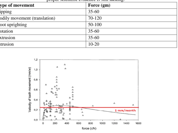
Table 2: Summary of guidelines for recommended force levels for orthodontic movement. Adapted from Proffit 4th Ed (Proffit et al., 2007) *Note, these are merely guidelines, as
proper scientific evidence is still lacking.
Type of movement Force (gm)
Tipping 35-60
Bodily movement (translation) 70-120
Root uprighting 50-100
Rotation 35-60
Extrusion 35-60
Intrusion 10-20
Figure 1: Summary of clinical data for velocity of tooth movement versus force (Ren et al., 2004).
I.v. Current mechanical prediction of orthodontic loading and its limitations From a mechanical perspective, orthodontic force systems can be very complex, typically including 14 teeth and brackets per arch. With this many deflections in an
predict force levels using free-body diagrams and the principles of statics. Additionally, the contribution of friction and binding to the force system is difficult to predict.
As previously discussed, Ren et al. (2003) concluded in a recent systematic review that no ideal force level could be recommended in orthodontics based on the current literature. This may be due to the fact that current literature typically records merely the magnitude of space closure that results from an applied force level. Closer examination of the interaction between orthodontic force and tooth movement requires knowledge of how applied force creates stress and strain in the surrounding tissue, and full understanding of how the tooth moves in three planes of space under the applied load. Careful clinical studies and detailed impressions can record detailed tooth movement, but non-destructive in vivo techniques for measuring stress and strain in the PDL and surrounding bone do not exist.
An engineering technique known as finite element analysis (FEA), which uses the principles of solid mechanics on a virtual model, has been developed that can bridge this gap. This technique is growing in popularity in orthodontics, due to its ability to show internal strains and to solve statically indeterminate force systems ( Nikolai, 1975; Poppe et al., 2002; Cattaneo et al., 2005; 2009a; 2009b; Hohmann et al., 2009). However, the predictions from FEA depend greatly on the assumptions made in creating the model, especially properties of the PDL, contact conditions, and boundary conditions (Cattaneo et al., 2009a).
I.vi. Finite element analysis
technique that can accomplish this is known at finite element analysis (FEA). This technique divides a virtual structure into discrete elements. Specific material properties are applied, boundary conditions are set, and approximate solutions can be found using the Ritz method of numerical analysis (Jones et al., 2001). This method can directly calculate approximate solutions for the complex matrix of partial differential equations and associated boundary conditions set during FEA. The solution includes calculated stress and strain at any point within the geometry.
Although this technique was originally employed for relatively simple
two-dimensional (2D) objects, recent advances and technological improvements have allowed for more complex, three-dimensional (3D) geometries to be analyzed. The technique is growing in popularity in dentistry since its introduction by Farah in 1973 (Farah et al., 1973).
Currently, multiple complex dental models have been published, showing dramatic improvements over the roughly meshed 2D initial models. Recent advancements in
orthodontic FEA fall under two broad categories: improved modeling of biological structures and improved modeling of orthodontic appliances.
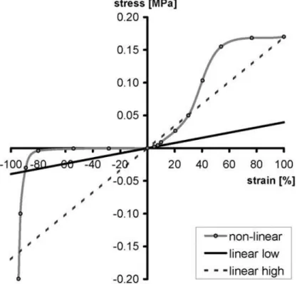
Multiple researchers have worked on improved modeling of biological structures. Probably the most significant studies were the series of papers published by Cattaneo between 2005 and 2009 (Cattaneo et al., 2005; 2008; 2009a; 2009b). In the initial study, sequential 2D layers from a μCT scan (37 micron voxel size) were stacked to create a high
different PDL properties were examined: a low stiffness linear modulus (0.044 MPa), a high stiffness linear modulus (0.17 MPa), and a non-linear modulus that was nearly zero under compression (Figure 2). The resulting stress in various levels of the PDL and alveolar bone was vastly influenced by whether a density-based modulus for bone utilizing the traced internal structure or a single averaged modulus for bone was used. Additionally, the different PDL assumptions were also found to vastly influence the resulting stress in the PDL and bone.
appeared to defy standard mechanical principles, but makes sense in terms of the non-linear PDL behavior used in the study (Figure 2), with minimal PDL stiffness initially in
compression.
The final study published by Catteneo’s group investigated the response of anterior
and posterior teeth under different loading conditions (Cattaneo et al., 2009b). Uncontrolled tipping, translation, and occlusal forces were tested separately on a two-tooth anterior and two-tooth posterior model. The traditional theory of distinct pressure and tension zones causing bone resorption and deposition, respectively, was not observed. Very little compressive stress was seen until the dentin nearly was touching the alveolar bone. However, this was due to the nonlinear assumption used in the study, with a very low Young’s Modulus for the PDL until the two surfaces were nearly touching. Interestingly,
little data on PDL strain was reported, which may have been more appropriate on the pressure side. Additionally, the authors tested a separate model using a generic block of bone as opposed to accurate geometry. They reported a significantly different stress distribution, highlighting the importance of anatomically accurate models.
In another study advancing the ability of FEA to model biological complexity, Jones et al attempted to correlate the in vivo tooth displacement allowed by the PDL with FEA properties (Jones et al., 2001). The clinical study was run very well, using a laser to measure tooth displacement in ten healthy volunteers with 0.39 N of load placed on the facial surface of the central incisor. Measurements were taken every 0.01 seconds, but the study was only run for one minute (10 seconds of pre-loading, 30 seconds of loading, and 20 seconds of relaxation), so the full extent of changes during orthodontic tooth movement was not
an approximate modulus of elasticity of 1 N/mm2 (1 MPa) and a Poisson’s Ratio of 0.45 for the PDL. The FEA was conducted using a generic model with a fairly rough mesh, but this remains one of the few studies to correlate in vivo findings with FEA results. Since
correlation with in vivo findings is essential to verifying the accuracy of FEA assumptions, this study remains valuable.
No previous studies analyzing orthodontic loading of the dentition using FEA have confirmed that true orthodontic loading can be modeled without the inclusion of accurate orthodontic appliances, yet accurate appliances are found infrequently in the literature. Several studies have examined torque control and center of resistance of incisors by placing loads directly onto the tooth structure, using a rough mesh, and keeping teeth bonded relative to each other ( Reimann et al., 2007; Liang et al., 2009). Some recent studies have added tooth attachments, although frequently they did not accurately mimic orthodontic brackets, but merely incorporated generic rectangular blocks (Field et al., 2009).
It appears from the results of recent studies that adding complexity and some appliance geometry will clearly influence results, but care must be taken to closely analyze how the appliances are used. A recent study using a rough bracket design compared orthodontic tooth loading using a single tooth and using a three-tooth model, finding
When examining FEA solutions, it is imperative to examine the mesh convergence as well. Unfortunately, few studies have examined this in dentistry and no studies have
examined the effects of mesh density in orthodontics. Two dental articles highlight the issues of using a single mesh size (Schmidt et al., 2009; Bright & Rayfield, 2011). Schmidt el al found dramatic issues with convergence of the maximum von-Mises stress when examining orthodontic miniscrews using implicit calculations (Schmidt et al., 2009). Convergence using the explicit solver, however, was obtained relatively quickly. Pull-out velocity of the miniscrew was found to influence mesh convergence, but density had a negligible effect. Bright and Rayfield examined a domestic pig skull meshed to 18 different densities (Bright & Rayfield, 2011). Forces were applied to the model at the insertion points of the temporalis and masseter muscles, modeling muscle loading of the skull structure. Linear and quadratic tetrahedral elements were both used and did not significantly alter the rate of convergence. Convergence typically occurred to within 5% by a 0.92 mm mesh sizing (total of 1,750,000 elements), but in some occasions occurred with as rough as a 2 mm mesh density (250,000 elements). Models with insufficient mesh density underestimated strain and displacement, leading to inaccurate results and conclusions. Both studies agree that mesh convergence is acceptable if < 5% variation occurs with further mesh refinements.
I.vii. Well-controlled clinical data on canine retraction.
Well controlled clinical data was obtained by Hayashi at the Health Sciences
University of Hokkaido, Japan. (Hayashi et al., 2006) This study consisted of 10 patients (4 males, 6 females, 19.4 – 29.2 years old), who required upper premolar extractions and retraction of maxillary canines with absolute anchorage. Osseointegrated midpalatal implants (Institute Straumann AG, Waldenburg, Switzerland) were used to provide anchorage. The implant was connected to the maxillary first molars through a 1.2 mm2 (~0.048” diameter) transpalatal arch with three steel ball bearings for fixed reference points
throughout treatment (Figure 3).
Figure 3: A. Clinical setup in Hayashi study (2006), with TPA placed with fixed reference points. B. Side view of clinical setup showing activation of NiTi coil spring.
Sliding mechanics were used for space closure. A 0.018” stainless steel continuous
gauge (Mitutoyo, Kawasaki, Japan). Each week the springs were reactivated to 12 mm to keep a constant force on the canine (either 0.5N or 1N).
Along with reactivating the appliances, hydrophilic vinyl polysiloxane impressions (JM Silicone, J. Morita, Tokyo, Japan) were taken every week. They were poured in die stone (Noritake super rock, J.Morita, Tokyo, Japan) and scanned with a slit laser beam (VMS-150RD, UNISN, Osako, Japan) to provide 3D digital models of the maxillary arch. The movement of the canine was measured from these virtual models using two different systems (Figure 4). In the XYZ system, the translation and rotation in all three planes of space (X, Y, and Z) were calculated as seen in Figure 4a. This method is relatively easy to understand for clinicians, as it highlights the movements and side effects in each direction. The other method calculated the finite helical axis (FHA) of the movement, as shown in Figure 4b. This is essentially the “center of rotation” for a 3D object. The calculated parameters are the direction vector of the helical axis (vx, vy, and vz), the rotation around the axis (θ), the translation around the axis (t), and the distance from the axis to the object (d).
Figure 4: The XYZ system (A) and FHA system (B) used by Hayashi to calculate tooth movement and side effects during canine retraction
(Hayashi, Uechi, Lee, & Mizoguchi, 2007).
The results from this study are shown in Table 3 (XYZ system) and Table 4 (FHA system). No difference in the amount of distal movement was seen between the 0.5N and 1N group. However, this study found increased distal tipping in the 1N group. Additionally, looking at the direction vector of the FHA, significant differences were seen in vx and vy, which essentially corresponds to tipping and flaring of the canine. These results clearly illustrated a biomechanical difference in retraction with 0.5N versus 1N of force. Table 3: XYZ clinical data from Hayashi et al (Hayashi et al., 2007)
XYZ system parameters 0.5 N 1.0 N P
Mean SD Mean SD
Distal Movement of canine crown tip (mm) 3.16 0.60 3.39 0.70 0.236 NS Tipping angle ψ of canine (degrees) 6.99 2.10 8.22 2.23 0.048 *
Flaring angle θ -1.39 2.12 -1.54 1.22 0.583 NS
Table 4: Finite Helical Axis (FHA) data from Hayashi et al (Hayashi et al., 2007).
FHA system parameters 0.5 N 1.0 N P
Mean SD Mean SD
Distal Movement of canine crown tip (mm) 3.17 0.60 3.38 0.71 0.199 NS Rotation around the FHA θ (degrees) 12.24 2.14 12.91 2.30 0.478 NS Translation along the FHA t (mm) 0.37 0.17 0.29 0.13 0.223 NS Shortest distance from the space coordinate
origin to the FHA d (mm)
14.63 7.54 14.74 8.01 0.877 NS Direction vector of the FHA vx -0.25 0.22 -0.57 0.20 0.048 * Direction vector of the FHA vy 0.61 0.21 0.37 0.22 0.042 * Direction vector of the FHA vz 0.61 0.29 0.58 0.30 0.234 NS *P < 0.05. NS, not significant.
Although this study provides excellent controlled clinical data, these results do not provide data on the stress and strain within the PDL and alveolar bone. Therefore,
comparing this data with an accurate FEM could further improve our understanding of orthodontic tooth movement.
I.viii. Hypothesis
We hypothesize that biomechanical parameters calculated from a finite element model of sufficient complexity can be correlated to well-controlled clinical data for tooth movement.
This study focused on four specific aims:
1. To create a complete maxillary biomechanical model capable of analyzing orthodontic canine retraction using absolute anchorage.
3. To determine the effects of model size, mesh sizing, accurate orthodontic appliances, and periodontal ligament linear elastic modulus on the resulting finite element predictions.
4. To compare calculated tooth movement during initial loading with controlled clinical data provided by Hayashi.
II. METHODS AND MATERIALS
II.i. Creation of a complete maxillary biomechanical model.
Construction of a working finite element model involves many steps and is especially difficult for organic objects. Many engineering models, such as cars or bridge trusses, can be directly created in a computer-engineering design (CAD) program. However, organic
structures are typically too complex to be created de novo in a CAD program. Rather, they must be reverse engineered by digitization of the organic structure itself. Currently,
computed tomography (CT) scans are the ideal method of acquiring this data. Optical laser scans are also common, but will only capture surface data.
For this study, accurate geometry for maxillary teeth was generated from micro-computed tomography (μCT) scans of previously extracted teeth without any unusual geometry, previous restorations, or decay present. The pulp, dentin, and enamel outlines were identified on sequential slices of the μCT scan and then stacked to create a solid body. The geometry of the supporting bone was determined from a previously obtained human cone-beam computed tomography (CBCT) scan with no evident bony pathology. Again, by examining sequential slices, the maxilla was differentiated into cortical bone, trabecular bone, and sinus.
irregularities and potential holes. A program capable of manipulating these polygons and creating solid CAD bodies is required, such as Geomagic (Geomagic USA, Morrisville, NC, USA)
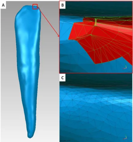
Although segmentations may initially appear very accurate (Figure 5a), there are often many small irregularities that must be addressed (Figure 5b). Obviously, organic objects will have natural irregularities that may be important to maintain, but defects from the scanning and segmentation process must be removed. Automated processes in Geomagic such as “mesh doctor” can identify problematic areas (Figure 5b) and fix many minor
Figure 5: Although initial geometry following segmentation can appear smooth (A), many small defects are present that Geomagic will highlight in red using "mesh doctor" as potentially problematic (B). Following closing gaps, smoothing, minor defeaturing, and
optimization for surfacing, the polygon mesh is greatly improved (C).
surfaces over to a FEA program for analysis without using a CAD program. This can be very effective for relatively simple models, but when multiple solid bodies are included and various mesh densities are required this process becomes cumbersome.
To use a CAD program with organic structures, a mathematical approximation of the surface must be generated from the polygon mesh surface. This is typically done with NURB surfaces, so the solid can be saved as in a standard .iges or .step file format. This process involves multiple steps – laying out patches, creating grids within these patches, optimizing the surface detail with grids, and finally creating the NURB surface (Figure 6, discussed in detail in Appendix 1). Surfacing must be done carefully, as incorrectly laying out the patches on the surface or not allowing sufficient detail may severely distort the surface. In the end, the surfaced body should be free of problematic geometry, such as sliver faces, small faces, or small edges.
Figure 6: Process of NURB surface generation using Geomagic. A. Contour lines are defined that follow the natural geometry - in this case, line angles were used. B. Patches were constructed and shuffled to create a clean grid pattern. C. Grids were created within each patch. D. NURB surfaces are created by placing control points along the created grids.
Therefore, the use of a genuine CAD program is typically preferred for detailed
characterization of the material and its contact correlation with surrounding structures. In
this study, Solidworks 2010 (Solidworks Corp., Concord, MA, USA) was utilized for all
CAD manipulation of the model – further details may be found in Appendix 2.
To model the appliances, 0° CAD brackets with accurate geometry will be placed on the facial surfaces of the teeth. A straight wire was placed through the brackets and virtual coil springs (0.5N and 1 N) to retract the canine were modeled by forces applied to the canine and molar bracket hooks. The interface between the wire and bracket was set to a contact mode, which is more difficult to model virtually than a bonded contact due to non-linear behavior and lack of corresponding nodes across the interface. However, it more accurately describes the interaction clinically. No previous studies could be found where this has been done for a half-maxilla model.
Figure 7 portrays the final half maxilla model, which incorporates the design features described above. Although Figure 7 initially appears similar to other finite element models shown in the literature, it provides several significant advantages over previous model designs, including:
It contains minimal problematic geometry. There are no sliver faces (very small in
one dimension), small edges (less than expected mesh size), flipped normals, or gaps. This enhances reliable meshing with various mesh sizes.
An ability to manipulate contact conditions and boundary conditions. The assembled
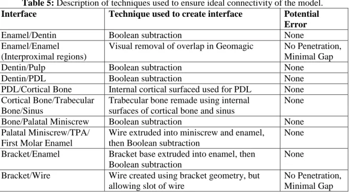
Ideal connectivity. Bodies were created to ensure ideal contact conditions as
summarized in Table 5.
Figure 7: Final half maxilla model created after smoothing and surfacing in Geomagic and CAD manipulation in Solidworks. Note the significant improvements of this model noted in
the text.
Table 5: Description of techniques used to ensure ideal connectivity of the model.
Interface Technique used to create interface Potential
Error
Enamel/Dentin Boolean subtraction None
Enamel/Enamel
(Interproximal regions)
Visual removal of overlap in Geomagic No Penetration, Minimal Gap
Dentin/Pulp Boolean subtraction None
Dentin/PDL Boolean subtraction None
PDL/Cortical Bone Internal cortical surfaced used for PDL None Cortical Bone/Trabecular
Bone/Sinus
Trabecular bone remade using internal surfaces of cortical bone and sinus
None
Bone/Palatal Miniscrew Boolean subtraction None Palatal Miniscrew/TPA/
First Molar Enamel
Wire extruded into miniscrew and enamel, then Boolean subtraction
None Bracket/Enamel Bracket base extruded into enamel, then
Boolean subtraction
None Bracket/Wire Wire created using bracket geometry, but
allowing slot of wire
No Penetration, Minimal Gap
Inc., Huston, PA, USA) was used for the FEA software. One desirable feature of this software is that it has a direct import tool from Solidworks, so no model detail is lost by saving into a different file format. Once in ANSYS, the model must be divided into a finite number of elements, known as the mesh, which can be analyzed. The model was meshed using 10-node tetrahedral h-elements (ANSYS solid 187), with an 8-node swept hexahedral mesh for the wire. Mesh parameters used for the complete model are shown in Table 6, and the created mesh is shown in Figure 8.
Table 6: Mesh sizing used for complete half maxilla model.
Part Body mesh sizing (mm)
Cortical bone, trabecular bone, miniscrew, TPA, and sinus
2.0
Brackets and wire 0.2
Enamel, dentin, pulp, and PDL 0.8
x-closely mimics a wire clinically that cannot travel around the arch perimeter but otherwise is unrestrained except for the brackets.
Reported material properties for cortical bone, trabecular bone, periosteum, gingiva, enamel, and dentin were applied to the finite element model (Table 7). The most difficult material to accurately model is the PDL. Assuming a linear, isotropic response uses the least computing power, but the PDL is actually a viscoelastic material. Previous studies have shown significant differences by using a non-linear response (Cattaneo et al., 2009b). Various assumptions for the PDL elastic modulus were tested to balance accuracy with realistic computational requirements (Table 8) (Poppe et al., 2002; Nekouzadeh et al., 2007; Qian et al., 2009). The various tests performed are described in further detail in Section II.iii.
Table 7: Material Properties for all materials in the model, except the PDL described in Table 8. Both the Poisson’s ratio and Young’s Modulus (Elastic Modulus, E) are reported. (Bourauel et al., 1999; Jones et al., 2001; Poppe et al., 2002; Toms et al., 2002; Toms et al., 2002; Toms & Eberhardt, 2003; Ziegler, Keilig, Kawarizadeh, Jager, & Bourauel, 2005)
Poisson's Ratio (v)
Young's Modulus (GPa)
Enamel 0.41 80
Dentin 0.31 18
Pulp 0.30 0.175
Cortical Bone 0.31 13.7
Trabecular Bone 0.30 1.37
Figure 9: Boundary conditions on the model – showing a fixed support placed on the central mirror plane. The mesial of the wire was also fixed in the x-dimension (unable to cross
midline), but no other boundary conditions were applied.
Figure 10: Five displacement probes set on the canine crown to record displacement of various regions of the tooth.
II.ii. Isolation of a two-tooth substructural model
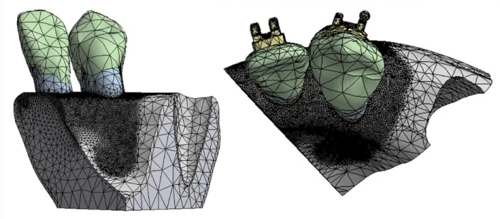
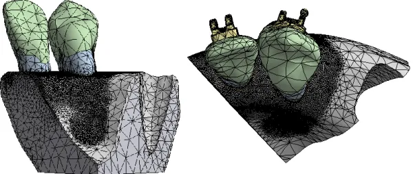
Figure 11: Limited-scope model with two teeth and fixed supports applied at both sectioned surfaces. In this model, the wire was suppressed.
Figure 12: Fine mesh for the limited model, generated with a 0.2mm contact sizing between the dentin and cortical bone.
II.iii. Effects of model size, mesh density, PDL properties, and accurate orthodontic appliances.
Four different parameters were varied to examine their effects on the final FEA results. The first parameter analyzed was model size. The complete half maxilla model (Section II.i.) was solved and the final displacement, maximum stress, and maximum strain were compared to the substructural two-tooth model (Section II.ii).
Next, the effect of mesh sizing was examined. Substructural models were solved using both a coarse and fine mesh size as described above. If a certain model would not solve due to computational requirement, all models of increased complexity were excluded.
Finally, many published values have been used to model the PDL (Cattaneo et al., 2005; Chen et al., 2005). Table 8 shows the four values used in this study.
Table 8: Different Poisson’s Ratio (v) and Young’s Modulus (E) Values used for the PDL v E (MPa)
Chen et al. 0.30 1750
Finally, the complete model and substructural model were both generated with full orthodontic appliances and a passive 0.018” SS wire, but each model was run both with the
wire in place and after suppressing the wire (fully removing the wire from the FE analysis). This tested whether placing accurate orthodontic appliances significantly altered FEA results.
II.iv. Comparison of FEA results with clinical data
Solutions were obtained in initial loading during sliding mechanics under 0.5 N and 1.0 N force. Differences between these two models were compared both qualitatively and quantitatively. Visually, strain distributions were compared between simulations and the movements found in the clinical data by Hayashi presented in Section I.vii.
III. Results
III.i. Specific Aim 1: Creation of a complete maxillary biomechanical model The specific aim of creating a full maxillary biomechanical model capable of analyzing orthodontic canine retraction using absolute anchorage was achieved. This
complete model was named the FJORD model (Full Jaw Orthodontic Dentition model, UNC copyright, Ko Lab 2011). Forty-three solid bodies were resurfaced, confirming seamless interfaces. This model properly integrates with current versions of Solidworks (Version 2010) and ANSYS (Version 13.0) with no reported error messages during transfer. Although the entire model was too large to be considered a single multi-body part that can undergo conformal meshing (meshing all aspects of the model at one time, given coincident nodes at interfaces), the 43 solid bodies were able to be grouped into 8 multi-body parts: each tooth (with pulp, dentin, enamel, bracket, and PDL), the surrounding bone, and the archwire. Interfaces between bodies were checked, showing no significant gaps or penetration – except where clinically realistic gaps were desired between the bracket and wire (frequently referred to as slop). Mesh variations and non-linear interface conditions (e.g. friction and
Figure 13: Solved full half maxilla model showing total deformation during canine retraction with 1.0 N of force. Model was solved with an 0.018” SS archwire with frictionless interfaces. Note the minimal deformation of the molar, indicating successful anchorage with
the palatal implant.
Converged FE solutions also include a full stress and strain components for each node – these results can be displayed graphically. Figure 14 shows von-Mises (equivalent) elastic
strain over the whole model, showing increased strain on the canine and molar hooks where the model was loaded and also within the canine PDL. Minimal strain was seen in the molar PDL, as would be expected with the presence of the transpalatal arch to the palatal
Figure 14: Equivalent (von-Mises) elastic strain in the full model during retraction with 1.0 N of force. PDL stiffness was set at 1750 MPa. (No archwire was included as the wire did
not engage at this PDL stiffness).
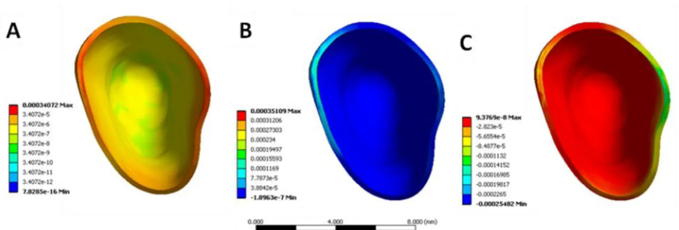
Individual bodies can also be examined after the model has solved. Figure 15 displays von-Mises (A), maximum (B), and minimum strain (C) in the canine PDL. These results were taken from the same model as Figure 14 - run under 1.0 N of retraction force and a PDL stiffness of 1750 MPa. Strain is seen on both sides of the PDL when looking at the equivalent strain, but tension is occurring on the mesial (Figure 15B) and compression on the distal (Figure 15C).
Figure 15: Equivalent (von-Mises) elastic strain (A), maximum elastic strain (B), and minimum elastic strain (C) within the canine PDL during retraction with 1.0 N of force.
III.ii. Specific Aim 2: Isolation of a two-tooth substructural model
The two-tooth substructure model isolated from the complete half maxilla model allows more complex analysis of canine movement, such as variations to PDL stiffness, mesh density, and contact conditions. While the full model was unable to converge on a solution when using a PDL stiffness <175 kPa, this substructure model was able to converge using a stiffness of only 44 kPa and have sufficient computational resources (16GB) to solve at a higher mesh. This model, including especially the fine PDL mesh, is shown in Figure 16.
Figure 16: Isolated two-tooth substructure from the full half maxilla model, demonstrating the fine PDL mesh size.
III.iii. Specific Aim 3: Effects of model size, mesh density, PDL properties, and accurate orthodontic appliances
Table 9 shows models tested with variations in mesh density, PDL properties, and orthodontic appliances. Solution time varied, with multiple comprehensive models unable to converge on a solution. High mesh density, low PDL stiffness, and the presence of
stiffness leads to greater deformation of the tooth, and additional appliances and interfaces will demand greater computational resources. Interestingly, orthodontic appliances produced almost no increase in solution time with a PDL modulus of 1,750 MPa, quadrupled solution time at 17.5 MPa, and increased over twenty times at 0.0175 MPa. Figure 17 shows that the canine does not tip enough to engage a round 0.018” archwire with any PDL stiffness, but a
large rectangular wire (0.022 x 0.020”) will engage at a 17.5 MPa stiffness (Note that archwire width was only 0.020” due to passive steel ligatures already in place on the
brackets). Engagement of the archwire dramatically increased computational requirements. Also of note was the fact that the high density mesh with the isolated two-tooth model had faster solution times than a course mesh on the complete model.
Table 9: Chart of time (seconds) required for models to converge, with models unable to converge marked with “DNC” (Did not converge).
Elastic Modulus Complete Model Complete Model Complete Model Partial Model Partial Model Partial Model
Pa Coarse Mesh Coarse - Wire Fine Mesh
Coarse Mesh
Coarse -
Wire Fine Mesh
1.75E+09 3531 s 3590 s DNC 181 s 254 s 1023 s
1.75E+07 6190 s 25456 s DNC 499 s 685 s 2419 s
1.75E+05 DNC DNC DNC 1943 s 117117 s 4429 s
Figure 17: Facial (A) and distal (B) view of the tipping of the maxillary canine under 1.0 N of force with a PDL stiffness of 1750 MPa. Note no engagement of the archwire due to
insufficient initial tipping.
Although adding complexity to the model increases solution time, these added
complexities should be included if they create significant changes to the prediction of clinical outcomes. Typically, in FEA, results between two models are considered equivalent if they vary by <5% ( Schmidt et al., 2009; Bright & Rayfield, 2011). Therefore, added mesh refinement, model size, and appliances that do not change the results by >5% are not
necessary to include for accurate results. Table 10 compares a fine mesh to a coarse mesh for displacement in the substructure model, showing significant variations for nearly all testing conditions (all except the cusp tip displacement with a 1750 MPa PDL stiffness).
Table 10: Comparison of a coarse mesh (CM) with a fine mesh (FM) in the two-tooth limited model of canine retraction with four different values for linear elastic modulus (E). Maximum displacement (Dmax) and overall displacement of the canine cusp tip (Cusp) are
included.
PDL E Dmax Dmax % Cusp Cusp %
(MPa) CM - mm FM - mm CM - mm FM - mm
1750 2.84E-03 2.60E-03 9.48 4.85E-04 4.86E-04 -0.06 17.5 4.74E-03 4.28E-03 10.67 2.43E-03 2.24E-03 8.44 0.0175 0.16115 0.13362 20.60 0.14051 0.11508 22.10 0.0044 0.62956 0.56455 11.52 0.5489 UNCONVERGED Table 11: Comparison of a coarse mesh (CM) with a fine mesh (FM) in the two-tooth limited model of canine retraction with four different values for linear elastic modulus (E).
Maximum stress (Stress max) and maximum strain (Strain max) of the canine cusp tip are included.
PDL E Stress max Stress Max % Strain max Strain max %
(MPa) CM - MPa FM - MPa CM FM
1750 79.296 53.961 -46.95 3.96E-04 2.70E-04 -46.95 17.5 79.296 53.961 -46.95 3.71E-03 4.16E-03 10.65 0.0175 79.295 53.961 -46.95 0.28709 0.30673 6.40
0.0044 79.293 UNCONVERGED 1.085 UNCONVERGED
Therefore, if computational resources are limited, it would appear that a slightly smaller model with a finer mesh may provide more accurate results.
Table 12: Comparison of the two-tooth partial model (PM) and the six-tooth half maxilla (HM) for modeling canine retraction with two different values for linear elastic modulus (E).
Maximum displacement (Dmax) and overall displacement of the canine cusp tip (Cusp) are included.
PDL E Dmax Dmax % Cusp Cusp %
(MPa) PM - mm HM - mm PM - mm HM - mm
1750 2.84E-03 2.84E-03 0.06 4.85E-04 4.98E-04 -2.61 17.5 4.74E-03 4.97E-03 -4.66 2.43E-03 2.69E-03 -9.76 Table 13: Comparison of a two-tooth partial model (PM) and a six-tooth half maxilla (HM)
for modeling canine retraction with two different values for linear elastic modulus (E). Maximum stress (Stress max) and maximum strain (Strain max) of the canine cusp tip are
included.
PDL E Stress max Stress Max % Strain max Strain max %
(MPa) PM - MPa HM - MPa PM HM
1750 79.296 68.144 16.37 3.96E-04 3.41E-04 16.37 17.5 79.296 68.143 16.37 3.71E-03 3.49E-03 6.47 Solutions obtained using models with accurate orthodontic appliances were also
compared to models without orthodontic archwires in place. It was found that for a PDL stiffness ≥17.5MPa, no bracket-to-wire interaction occurred, so modeling the appliances was
not required if testing a high stiffness PDL during initial loading. In fact, when the original 0.018” stainless steel archwire was placed in the model, it did not engage the brackets under
any loading conditions tested. When moving to the larger rectangular wire, engagement did occur with a PDL stiffness of either 0.044 MPa or 0.175 MPa.
Figure 18: Resultant force (A) and moment (B) felt by the PDL during canine retraction at any force level without orthodontic appliances. This shows a resultant force in the PDL predominantly in the distal direction. The resultant moment shows tipping and rotation are both occurring. *Note: These directions are identical at any force level, as opposed to Figure
19 and 20 with orthodontic appliances.
Figure 19: Resultant force during canine retraction with 0.5 N (A) and 1.0 N (B) when modeling orthodontic appliances.
Figure 20: Resultant moment during canine retraction with 0.5 N (A) and 1.0 N (B) when modeling orthodontic appliances (PDL=0.175 MPa)
III.iv. Specific Aim 4: Comparison with clinical data
FEA, as shown in Figure 19 and 20. Table 14 shows the FHA parameters calculated by Hayashi, as well as results found in this study. Interestingly, the values for vz were roughly similar, corresponding to the degree of rotation present. However, the values for vx and vy were quite different from the data found clinically. The overall degree of rotation about the FHA was ~1% of rotation found in the clinical data. Therefore, properly modeling the resultant direction of tooth movement requires remodeling of the FE model.
Table 14: Comparison of the FHA clinical data for canine retraction provided by Hayashi and the generated results from FEA under 0.5 N and 1.0 N of load.
FHA system parameters 0.5 N 1 N P 0.5 N 1 N
Mean SD Mean SD FEA FEA
Distal movement of canine crown tip (mm)
3.17 0.6 3.38 0.71 0.199 NS 0.0215 0.0685
Rotation around the FHA θ (degrees)
12.24 2.14 12.91 2.3 0.478 NS -0.275 -0.226
Translation along the FHA t (mm)
0.37 0.17 0.29 0.13 0.223 NS 0 0
Shortest distance from the space coordinate
14.63 7.54 14.74 8.01 0.877 NS
origin to the FHA d (mm)
Direction vector of the FHA vx -0.25 0.22 -0.57 0.2 0.048 * 0.731 0.680
Direction vector of the FHA vy 0.61 0.21 0.37 0.22 0.042 * -0.127 -0.0864
Direction vector of the FHA vz 0.61 0.29 0.58 0.3 0.234 * 0.671 0.728
IV. DISCUSSION
IV.i. Comparison of Results to Previous Literature
This study provides the first known report in the literature of a complete maxillary biomechanical model combining high-quality tooth geometry and accurate orthodontic appliance placement, while maintaining independent anatomy (enamel, dentine, pulp, PDL, and alveolar bone can all be separately manipulated) and high-quality interfaces capable of mesh size variations and interface manipulation (e.g. bonded contacts, frictionless contacts).
Cattaneo et al. has shown the importance of high-quality μCT scans of the dentition and creation of a high-quality virtual model (Cattaneo et al., 2005; 2008; 2009a; 2009b), yet point forces and moments are not capable of representing the wide variety of tooth loading conditions available with the FJORD model. Additionally, these studies included only two teeth, while our results highlighted differences when moving to a full half maxilla with contact interfaces between neighboring teeth.
average PDL stiffness of 0.175 MPa (the high stiffness PDL model described by Cattaneo, 2005), increasing the mesh density of the PDL altered displacement results by 20.6%, stress by 47.0% and strain by 6.4%. Less than 5% variation is typically required to assume model convergence and therefore accurate results. Therefore, a single element thickness in the PDL was not sufficient for mesh convergence in this study.
The current comprehensive FJORD model is the first reported model to provide sufficient anatomical accuracy for reliable biomechanical modeling of a full jaw, while maintaining independent CAD bodies capable of variations in meshing. Our results show, however, that high density meshes demand substantial computational resources when implemented on a full model. This led to many results being generated through the use of a limited two-tooth model. However, as opposed to other limited models published in the literature, the accuracy of our limited model was demonstrated through comparison with the comprehensive model.
IV.ii. FEA versus Laboratory Testing
Some authors have criticized the use of finite element modeling in orthodontics due to lack of complete validation for each model and loading condition. While model validation is important, the mechanical principles underlying the analysis are mathematically valid (Timoshenko & Goodier, 1951; Lanczos, 1962;). Therefore, it is important to examine the assumptions made and the interaction of mesh density (mathematical convergence), but once these assumptions are validated, the technique can be widely applied in orthodontics.
industries is first performed with computer simulations. This is extremely effective for the automotive and aeronautic industries due to the high cost of producing designs for laboratory testing. In orthodontics, the progression to computer modeling is also extremely important, as it is the only way to examine biological structures and internal stresses without destructive evaluation of tissues.
A currently advocated laboratory technique for quantification of resulting forces from a statically indeterminate system uses force and torque transducers attached to brackets in an orthodontic arch (Badawi et al., 2009). While this method can provide a great deal of
valuable information on resultant forces and moments, it does have major limitations. The first concern is the absence of biological tissues from the analysis, especially the PDL. Without the PDL, it is impossible to extrapolate the data to the human conditions of tooth movement. Therefore, the effects of initial displacement of the teeth under loading and the long-term viscoelastic effects within the PDL cannot be examined.
The second major concern using a laboratory model is that currently available force and torque transducers still are relatively large when compared to orthodontic brackets. Therefore, the transducers must be placed a distance away with a cantilever arm to the bracket (Figure 21). This cantilever arm is affected by loading and the deformation
Figure 21: Laboratory model used by Badawi et al (Badawi et al., 2009).
Finally, the greatest limitation of this technique is that even if forces and moment can be accurately determined, the resulting stress and strain within the tissue cannot be
calculated. As discussed in Section I, further advancements in orthodontics require more accurate characterization of the effect of loading. Only calculation of internal stress and strain will be able to separate the effects of PDL and alveolar bone loading, determine how specific stress and strain corresponds to biological response, and how this affects tooth movement.
Full validation of FEA in orthodontics is ongoing, but a great deal of progress has been made by several investigators. Jones et al. compared initial loading of an incisor with a FE model of an incisor, showing an appropriate elastic modulus of 1 MPa and Poisson’s Ratio of 0.45 (Jones et al., 2001). Catteneo et al. explored the importance of non-linear viscoelastic effects and accurate representation of alveolar bone anatomy (Cattaneo et al., 2009b). The importance of modeling multiple teeth was shown by Field et al (Field et al., 2009). Our findings highlight the importance of accurate appliances and proper mesh
excellent guidelines for creation of FE models capable of producing data translatable to clinical application.
IV.iii. Current Limitations and Further Improvements
Although the FJORD model is a significant improvement in orthodontic FEM, limitations still exist. One of the primary limitations is current computational resources. In the 1970s and 1980s, 3D modeling was rarely performed due to computational demands. The vast improvement in computer speed and memory in the last few decades has allowed the development of accurate 3D models capable of modeling non-linear surface interactions. Despite these improvements, fine mesh sizes and comprehensive models can quickly strain computational resources. As processor speed, available RAM, and ability for parallel processing improves, model complexity can be further improved. It is important to note that the goal of FEA is not creation of the most complex model. Limited models are important, but must be validated against more complex ones to ensure no loss of accuracy. The current literature in orthodontics and this study both support the development of additional model complexity, as variation with further refinement still appears significant.
Degrees of Freedom
were combined into a multi-body part, while the cortical bone, trabecular bone, and sinus formed an additional part. This improved the mesh, but still leaves unmatched nodes at the interface between the PDL and cortical bone. When it attempts to create shared nodes at this interface, it effectively required the computer to mesh all parts simultaneously, which quickly exceeds the computational ability of our computer. Figure 22A shows minor variations that occur within the PDL when this occurs. Using a limited model, the computational ability is not exceeded, allowing matched nodes as seen in Figure 22B. Further improvements in computational ability and software capabilities may soon solve this issue.
Figure 22: A. Variations in the PDL surface arising from unmatched nodes. B. Smooth surface if the nodes are matched.
Contact Interfaces
coefficient of 0.2. However, increasing this coefficient or the size of the model led to unconverged solutions.
Another difficulty with current FEA modeling is a limited ability to model active ligation. The current study uses passive stainless steel ties on the mesial and distal to hold the wire into the slot. However, current tools in Solidworks do not allow the user to specify direct contact between the wire and ligature, nor a specific gap. Therefore, the ligatures are visually placed with minimal gap. Although reasonably accurate, some variation in
placement undoubtedly exists. Moving from passive ligation to active ligation introduces a great deal of added complexity. (A relatively simple method of applying a seating force on the wire at each bracket could be used. However, this force remains constant during modeling regardless the position of the wire to the base of the bracket, which does not accurately represent what occurs in a clinical situation.) In order to create a true active appliance, the birth-death technique introduced by Canales et al. must be utilized (Canales et al., In preparation). This greatly increases complexity and had not been previously attempted in the literature.
PDL
V. CONCLUSIONS
1. A comprehensive biomechanical model of the maxilla was developed capable of convergence under a variety of loading conditions.
2. A limited two-tooth model was extracted from the comprehensive model, allowing more complex simulations to converge with shorter solution times. However, predicted stress and strain values deviated from the full model by up to 16.4%. 3. Models with a single element PDL thickness were not fully converged, with up to
22% variation seen in displacement and 47% seen in stress when moving up to a fine mesh density with a two element PDL thickness.
4. The PDL elastic modulus significantly influenced the initial displacement, which can be used to partially describe the viscoelastic behavior of the PDL.
APPENDIX 1 GEOMAGIC i. Importing into Geomagic
Geomagic Studio is a powerful tool to accurately manipulate 3D scans into CAD models. In order to manipulate objects in Geomagic, the geometry must be imported from an external file. This could be an .stl file generated directly from a 3D scan, but for the
purposes of this study, .iges files were used since the geometry had already been converted to a CAD object previously. The .iges file type is one of the earliest developed file structures that is currently used – this provides a robust format, but lacks support for many complex functions (e.g. maintaining hierarchy, support for complex multibody parts). The dentin for the UL2 and for the UL5 both did not transfer properly using .iges, but the geometry was accurately transferred through the use of a .step file (a newer file version which interestingly had issues with multiple other surfaces in the model).
CAD files, such as .iges or .step, are displayed under the “CAD” tab once they are
imported into Geomagic. Since Geomagic is not a CAD program with multiple functions for surfaced objects, the first step is converting the geometry to a polygon model (Figure 23). ii. Manipulation of the Polygon Model
Figure 23: Polygon model of UL2 in Geomagic directly after importing from STEP file and converting to polygons.
Figure 24: To remove extra boundaries, first the click “Remove” under the “Boundary tab” and select “Clear Subdivision Points” (A). Next, select “Remove Boundary” and select any unwanted boundaries. Typically, it helpful to leave the apex boundary, because then the
bounded components can be selected (B). This can highlight the entire interior surface, which then can be moved into a new object, by selecting
Figure 25: Interior surface cut into a new object (PulpUL2) and the exterior dentin selected. Note: This view highlights that although the overall view may look nice, defects exist that
must be repaired.
Once the interior surface is cut away, typically it is preferred to fill the apex. This can be done by selecting “Fill single”, highlighting the option to fill by using the surrounding
Figure 26: Filling an open hole in Geomagic. Select “Fill single”, select the middle option (highlighted by a red square for emphasis) that fills the void by using the surrounding surface
normals, and click the hole that needs to be filled. Pressing Esc will exit the menu.
Although Figure 23 looks smooth and complete, Figure 26 shows that rough areas exist with regions where the surface normal is reversed (yellow polygons). A Geomagic tool known as “Mesh Doctor” will highlight problematic areas (Figure 27). While the Mesh
Figure 27: The “Mesh Doctor” tool highlights problematic geometry and offers automated repair options.
Figure 28: Defeaturing removes selected polygons and recreates the surface using the surrounding geometry. This work well to get rid of extremely rough geometry, but selection
Once rough areas are defeatured, mesh doctor can be used to automatically repair minor issues. The goal at the end of this stage is to have no errors occur under the
“Analysis” box of mesh doctor (Figure 29). Despite no problematic polygons, the geometry
is still not fully prepared for surfacing. Under the “Display” menu on the left there is an option to display “Edges”. After clicking this option, it is evident that many polygons near
the incisal edge are skewed and larger than the average polygons in the body. To fix the issue with the large polygons, the polygons can be selected and the “Refine Polygons” tool is
selected to increase polygon density (Figure 30). At this stage, the number of polygons in the overall model should be on the order of 200,000 to 400,000.
Figure 30: These selected polygons near the incisal edge are large and skewed. The “Refine Polygons” menu is open to create additional polygons in this area to improve the surface
mesh.
After modifying the polygon size, the surface can be smoothed through the use of the “QuickSmooth” command under the “Smooth” menu. Finally, the “Enhance Mesh for Surfacing” tool is used to create an ideal polygon distribution for surfacing (Figure 31).
Figure 31: “Enhance Mesh for Surfacing” tool that creates an ideal mesh distribution to create non-skewed elements to assist with ideal surfacing.
iii. NURB Surfacing
At this point, the polygon model is ready for NURB (Non-Uniform Rational B-spline) surfacing. To summarize, the object should be a smooth, continuous, closed surface made of non-skewed polygons. All surface normals should be facing the exterior (denoted by a blue surface in Geomagic) and the model should contain approximately 200,000 to 400,000 polygons. In case the polygon model requires further manipulation, it would be wise to save the file separately at this point and also create a copy of the object in the
Figure 32: Object copied and moved into “Exact Surfacing”. Initially, the menu has only the first box available, as shown in the red insert, but the rest of the options become available
once “Exact Surfacing” is clicked.
At this point, the first available option is for autosurfacing. Autosurfacing techniques are frequently used, but Figure 33 shows some issues that occur during autosurfacing. Figure 33-B shows the auto-detected contour lines, which clearly do not follow the true contours of this object. Based on these contour lines, a total of 302 patches are created for this surface. These patches become unique faces in Solidworks (although some time consuming