Multi-Agent Fully Decentralized Value Function
Learning with Linear Convergence Rates
Lucas Cassano, Kun Yuan and Ali H. Sayed
Abstract—This work develops a fully decentralized multi-agent algorithm for policy evaluation. The proposed scheme can be applied to two distinct scenarios. In the first scenario, a collection of agents have distinct datasets gathered following different behavior policies (none of which is required to explore the full state space) in different instances of the same environment and they all collaborate to evaluate a common target policy. The network approach allows for efficient exploration of the state space and allows all agents to converge to the optimal solution even in situations where neither agent can converge on its own without cooperation. The second scenario is that of multi-agent games, in which the state is global and rewards are local. In this scenario, agents collaborate to estimate the value function of a target team policy. The proposed algorithm combines off-policy learning, eligibility traces and linear function approximation. The proposed algorithm is of the variance-reduced kind and achieves linear convergence with O(1)memory requirements. The linear convergence of the algorithm is established analytically, and simulations are used to illustrate the effectiveness of the method.
Index Terms—Distributed reinforcement learning, policy eval-uation, temporal-difference learning, multi-agent reinforcement learning, reduced variance algorithms.
I. INTRODUCTION
T
HE goal of a policy evaluation algorithm is to estimate the performance that an agent will achieve when it follows a particular policy to interact with an environment, usually modeled as a Markov Decision Process (MDP). Policy evaluation algorithms are important because they are often key parts of more elaborate solution methods where the ultimate goal is to find an optimal policy for a particular task (one such example is the class of actor-critic algorithms – see [1] for a survey). This work studies the problem of policy evaluation in a fully decentralized setting. We consider two distinct scenarios.In the first case, K independent agents interact with inde-pendent instances of the same environment following poten-tially different behavior policies to collect data the objective is for the agents to cooperate. In this scenario each agent only has knowledge of its own states and rewards, which are independent of the states and the rewards of the other agents. Various practical situations give rise to this scenario, for example, consider a task that takes place in a large geographic area. The area can be divided into smaller sections, each of which can be explored by a separate agent. This framework is also useful for collective robot learning (see, [2]–[4]).
L. Cassano and K. Yuan are with the Department of Electrical Engineering, UCLA, CA 90095 USA e-mails:{cassanolucas,kunyuan}@ucla.edu.
A. H. Sayed is with the School of Engineering, Ecole Polytechnique Federale de Lausanne (EPFL), Switzerland. e-mail: [email protected].
The second scenario we consider is that of multi-agent reinforcement learning (MARL). In this case a group of agents interact simultaneously with a unique MDP and with each other to attain a common goal. In this setting there is a unique global state known to all agents and each agent receives distinct local rewards, which are unknown to the other agents. Some examples that fit into this framework are teams of robots working on a common task such as moving a bulky object, trying to catch a prey, or putting out a fire.
A. Related Work
Our contributions belong to the class of works that deal with policy evaluation, distributed reinforcement learning, and multi-agent reinforcement learning.
There exist a plethora of algorithms for policy evaluation such as GTD [5], TDC [6], GTD2 [6], GTD-MP/GTD2-MP [7], GTD(λ) [8], and True Online GTD(λ) [9]. The main feature of these algorithms is that they have guaranteed convergence (for small enough step-sizes) while combining off-policy learning and linear function approximation; and are applicable to scenarios with streaming data. They are also applicable to cases with a finite amount of data. However, in this latter situation, they have the drawback that they converge at a sub-linear rate because a decaying step-size is necessary to guarantee convergence to the minimizer. In most current applications, policy evaluation is actually carried out after collecting a finite amount of data (one example is the recent success in the game of GO [10]). Therefore, deriving algorithms with better convergence properties for the finite sample case becomes necessary. By leveraging recent developments in variance-reduced algorithms, such as SVRG [11] and SAGA [12], the work [13] presented SVRG and SAGA-type algorithms for policy evaluation. These algorithms combine GTD2 with SVRG and SAGA and they have the advantage over GTD2 in that linear convergence is guaranteed for fixed data sets. Our work is related to [13] in that we too use a variance-reduced strategy, however we use the AVRG strategy [14] which is more convenient for distributed implementations because of an important balanced gradient calculation feature.
Another interesting line of work in the context of distributed policy evaluation is [15], [16] and [17]. In [15] and [16] the authors introduce Diffusion GTD2 and ALG2; which are extensions of GTD2 and TDC to the fully decentralized case, respectively. While [17] is a shorter version of this work. These algorithms consider the situation where independent agents interact with independent instances of the same MDP.
These strategies allow individual agents to converge through collaboration even in situations where convergence is infeasi-ble without collaboration. The algorithm we introduce in this paper can be applied to this setting as well and has two main advantages over [15] and [16]. First, the proposed algorithm has guaranteed linear convergence, while the previous algo-rithms converge at a sub-linear rate. Second, while in some instances, the solutions in [15] and [16] may be biased due to the use of the Mean Square Projected Bellman Error (MSPBE) as a surrogate cost (this point is further clarified in Section II), the proposed method allows better control of the bias term due to a modification in the cost function. We extend our previous work [17] in four main ways which we discuss in the Contributionsub-section.
There is also a good body of work on multi-agent rein-forcement learning (MARL). However, most works in this area focus on the policy optimization problem instead of the policy evaluation problem. The work that is closer to the current contribution is [18], which was pursued simultaneously and independently of our current work. The goal of the formulation in [18] is to derive a linearly-convergent distributed policy evaluation procedure for MARL. The work [18] does not consider the case where independent agents interact with independent MDPs. In the context of MARL, our proposed technique has three advantages in comparison to the approach from [18]. First, the memory requirement of the algorithm in [18] scales linearly with the amount of data (i.e., O(N)), while the memory requirement for the proposed method in this manuscript is O(1)), i.e., it is independent of the amount of data. Second, the algorithm of [18] does not include the use of eligibility traces; a feature that is often necessary to reach state of the art performance (see, for example, [19], [20]). Finally, the algorithm from [18] requires all agents in the network to sample their data points in a synchronized manner, while the algorithm we propose in this work does not require this type of synchronization. Another paper that is related to the current work is [21], which considers the same distributed MARL as we do; although their contribution is different from ours. The main contribution in [21] is to extend the policy gradient theorem to the MARL case and derive two fully distributed actor-critic algorithms with linear function approximation for policy optimization. The connection between [21] and our work is that their actor-critic algorithms require a distributed policy evaluation algorithm. The algorithm they use is similar to [15] and [16] (they combine diffusion learning [22] with standard TD instead of GTD2 and TDC as was the case in [15] and [16]). The algorithm we present in this paper is compatible with their actor-critic schemes (i.e., it could be used as the critic), and hence could potentially be used to augment their performance and convergence rate.
Our work is also related to the literature on distributed optimization. Some notable works in this area include [22]– [32]. Consensus [23] and Diffusion [22] constitute some of the earliest work in this area. These methods can converge to a neighborhood around, but not exactly to, the global minimizer when constant step-sizes are employed [24], [32]. Another family of methods is based on distributed alternating direction method of multipliers (ADMM) [25]. While these methods
can converge linearly fast to the exact global minimizer, they are computationally more expensive than previous methods since they need to optimize a sub-problem at each iteration. An exact first-order algorithm (EXTRA) was proposed in [26] for undirected networks to correct the bias suffered by con-sensus, (this work was later extended for the case of directed networks [29]). EXTRA and DEXTRA [29] can also converge linearly to the global minimizer while maintaining the same computational efficiency as consensus and diffusion. Several other works employ instead a gradient tracking strategy [27], [28], [33]. These works guarantee linear convergence to the global minimizer even when they operate over time-varying networks. More recently, the Exact Diffusion algorithm [30], [31] has been introduced for static undirected graphs. This algorithm has a wider stability range than EXTRA (and hence exhibits faster convergence [31]), and for the case of static graphs is more communication efficient than gradient tracking methods since the gradient vectors are not shared among agents. Our current work closely related to Exact Diffusion since our MARL model is based on static undirected graphs and our distributed strategy is derived in a similar manner to Exact Diffusion. We remark that there is a fundamental difference between the algorithm we present and the works in [22]–[32], namely, our algorithm finds the global saddle-pointin a primal dual formulation while the cited works solve convex minimization problems.
B. Contribution
The contribution of this paper is twofold. In the first place, we introduceFast Diffusion for Policy Evaluation (FDPE), a fully decentralized policy evaluation algorithm under which all agents have a guaranteed linear convergence rate to the minimizer of the global cost function. The algorithm is de-signed for the finite data set case and combines off-policy learning, eligibility traces, and linear function approximation. The eligibility traces are derived from the use of a more general cost function and they allow the control of the bias-variance trade-off we mentioned previously. In our distributed model, a fusion center is not required and communication is only allowed between immediate neighbors. The algorithm is applicable both to distributed situations with independent MDPs (i.e., independent states and rewards) and to MARL scenarios (i.e., global state and independent rewards). To the best of our knowledge, this is the first algorithm that combines all these characteristics. Our second contribution is a novel proof of convergence for the algorithm. This proof is challenging due to the combination of three factors: the distributed nature of the algorithm, the primal-dual structure of the cost function, and the use of stochastic biased gradients as opposed to exact gradients.
This work expands our short work [17] in four ways. In the first place, in that work we used the MSPBE as a cost function, while in this work we employ a more general cost function. Second, we include the proof of convergence. Third, we show that our approach applies to MARL scenarios, while in our previous short paper we only discussed the distributed policy evaluation scenario with independent MDPs. Finally in this paper we provide more extensive simulations.
C. Notation and Paper Outline
Matrices are denoted by upper case letters, while vectors are denoted with lower case. Random variables and sets are denoted with bold font and calligraphic font, respectively.
ρ(A) indicates the spectral radius of matrix A. IM is the
identity matrix of size M. Eg is the expected value with
respect to distribution g. k·kD refers to the weighted matrix
norm, whereD is a diagonal positive definite matrix. We use
to denote entry-wise inequality. col{v(n)}N
n=1 is a column
vector with elements v(1) through v(N) (where v(N) is at the bottom). Finally R and N represent the sets of real and natural numbers, respectively.
The outline of the paper is as follows. In the next section we introduce the framework under consideration. In Section III we derive our algorithm and provide a theorem that guarantees linear convergence rate. In Section IV we discuss the MARL setting. Finally we show simulation results in Section V.
II. PROBLEMSETTING
A. Markov Decision Processes and the Value Function We consider the problem of policy evaluation within the traditional reinforcement learning framework. We recall that the objective of a policy evaluation algorithm is to estimate the performance of a known target policy using data generated by either the same policy (this case is referred as on-policy), or a different policy that is also known (this case is referred as off-policy). We model our setting as a finite Markov Decision Process (MDP), with an MDP defined by the tuple (S,A,P,r,γ), where S is a set of states of size S=|S|, A is a set of actions of size A=|A|, P(s0|s,a) specifies the probability of transitioning to state s0∈ S from state s∈ S
having taken action a∈ A, r:S×A×S →R is the reward function r(s,a,s0) when the agent transitions to state s0∈ S
from state s∈ S having taken actiona∈ A), and γ∈[0,1) is the discount factor.
Even though in this paper we analyze the distributed sce-nario, in this section we motivate the cost function for the single agent case for clarity of exposition and in the next section we generalize it to the distributed setting. We thus consider an agent that wishes to learn the value function,
vπ(s), for a target policy of interestπ(a
|s), while following a potentially different behavior policyφ(a|s). Here, the notation
π(a|s)specifies the probability of selecting actionaat states. We recall that the value function for a target policyπ, starting from some initial states∈ S at timei, is defined as follows:
vπ(s) =EP,π X∞ t=i γt−ir(st,at,st+1) si=s (1) wherestandatare the state and action at timet, respectively.
Note that since we are dealing with a constant target policyπ, the transition probabilities between states, which are given by
pπ
s,s0=EπP(s0|s,a), are fixed and hence the MDP reduces to
a Markov Rewards Process. In this case, the state evolution of the agent can be modeled with a Markov Chain with transition matrix Pπ whose entries are given by(Pπ)
ij=pπi,j.
Assumption 1. We assume that the Markov Chain induced by the behavior policy φ(a|s) is aperiodic and irreducible.
In view of the Perron-Frobenius Theorem [32], this condition guarantees that the Markov Chain under φ(a|s) will have a steady-state distribution in which every state has a strictly positive probability of visitation [32].
Using the matrix Pπ and defining: vπ=col{vπ(s)}Ss=1, rπ(s)=Eπ,P r(s,a,s0)
, rπ=col{rπ(s)}Ss=1 (2) we can rewrite (1) in matrix form as:
vπ=
∞
X
n=0
(γPπ)nrπ= (I−γPπ)−1rπ (3) Note that the inverse(I−γPπ)−1always exists; this is because γ <1 and the matrix Pπ is right stochastic with spectral radius equal to one. We further note thatvπ also satisfies the followingh−stage Bellman equation for anyh∈N:
vπ= (γPπ)hvπ+
h−1
X
n=0
(γPπ)nrπ (4)
B. Definition of cost function
We are interested in applications where the state space is too large (or even infinite) and hence some form of function approximation is necessary to reduce the dimensionality of the parameters to be learned. As we anticipated in the introduction, in this work we use linear approximations1. More formally, for every state s∈ S, we approximate vπ(s)≈xTsθ? where xs∈RM is a feature vector corresponding to statesandθ?∈
RM is a parameter vector such that M
S. Defining X= [x1,x2,···,xS]T∈RS×M, we can write a vector approximation
forvπ as vπ
≈Xθ?. We assume thatX is a full rank matrix;
this is not a restrictive assumption since the feature matrix is a design choice. It is important to note though that the truevπ
need not be in the range space ofX. Ifvπis in the range space
ofX, an equality of the formvπ=Xθ?holds exactly and the
value of θ? is unique (because X is full rank) and given by θ?=(XTX)−1XTvπ. For the more general case wherevπ is not
in the range space ofX, then one sensible choice forθ? is: θ?= argmin
θ k
Xθ−vπk2D= (XTDX)−1XTDvπ (5) where D is some positive definite weighting matrix to be defined later. Although (5) is a reasonable cost to define θ?,
it is not useful to derive a learning algorithm since vπ is not
known beforehand. As a result, for the purposes of deriving a learning algorithm, another cost (one whose gradients can be sampled) needs to be used as a surrogate for (5). One popular choice for the surrogate cost is the MSPBE (see, e.g., [6], [7], [15], [16]); this cost has the inconvenience that its minimizer θo is different from (5) and some bias is
1We choose linear function approximation, not just because it is
math-ematically convenient (since with this approximation our cost function is strongly convex) but because there are theoretical justifications for this choice. In the first place, in some domains (for example Linear Quadratic Regulator problems) the value function is a linear function of known features. Secondly, when policy evaluation is used to estimate the gradient of a policy in a policy gradient algorithm, the policy gradient theorem [34] assures that the exact gradient can be obtained even when a linear function is used to estimatevπ.
incurred [6]. In order to control the magnitude of the bias, we shall derive a generalization of the MSPBE which we refer to as H−truncated λ-weighted Mean Square Projected Bellman Error (Hλ-MSPBE). To introduce this cost, we start by writing a convex combination of equation (4) with different
h’s ranging from 1 toH (we chooseH to be a finite amount instead of H→ ∞ because in this paper we deal with finite data instead of streaming data) as follows:
vπ= (1−λ) H−1 X h=1 λh−1 (γPπ)hvπ+ h−1 X n=0 (γPπ)nrπ +λH−1 (γPπ)Hvπ+ HX−1 n=0 (γPπ)nrπ (6) = Γ2(λ,H)rπ+ρ1(λ,H)Γ1(λ,H)vπ (7) where we introduced: ρ1(λ,H)= (1−λ)γ+(1−γ)(γλ)H 1−γλ (8) Γ2(λ,H)= HX−1 n=0 (γλPπ)n= I−(γλPπ)H(I−γλPπ)−1 (9) Γ1(λ,H)= 1 ρ1(λ,H) (1−λ)γPπ HX−1 n=0 (γλPπ)n+(γλPπ)H (10) and0≤λ≤1is a parameter that controls the bias.
Remark 1. Note that0< ρ1(λ,H)≤γ <1.
Remark 2. Γ1(λ,H)is a right stochastic matrix because it is defined as a convex combination of powers ofPπ (which are right stochastic matrices).
Note that from now on for the purpose of simplifying the notation, we refer to ρ1(λ,H), Γ1(λ,H) andΓ2(λ,H)as ρ1,
Γ1 and Γ2, respectively. Replacing vπ in (7) by its linear
approximation we get:
Xθ≈Γ2rπ+ρ1Γ1Xθ (11)
Projecting the right hand side onto the range space of X so that an equality holds, we arrive at:
Xθ= Π[Γ2rπ+ρ1Γ1Xθ] (12)
where Π∈RS×S is the weighted projection matrix onto the
space spanned byX, (i.e.,Π =X(XTDX)−1XTD). We can now use (12) to define our surrogate cost function:
S(θ) =1 2 Π Γ2rπ+ρ1Γ1Xθ −Xθ 2 D+ η 2 θ−θp 2 U (13)
where the first term on the right hand side is the Hλ-MSPBE,
η≥0 is a regularization parameter, U >0 is a symmetric positive-definite weighting matrix, andθpreflects prior knowl-edge about θ. Two sensible choices for U are U=I and
U=XTDX=C, which reflect previous knowledge about θ
or the value functionXθ, respectively. The regularization term can be particularly useful when the policy evaluation algorithm is used as part of a policy gradient loop (since subsequent policies are expected to have similar value functions and the value of θ learned in one iteration can be used as θp in the next iteration) like, for example, in [35]. One main advantage
of using the proposed cost (13) instead of the more traditional MSPBE cost is that the magnitude of the bias between its minimizer (denoted as θo(H,λ)) and the desired solution θ?
can be controlled throughλandH. To see this, we first rewrite
S(θ)in the following equivalent form:
S(θ)=1 2 XTD(I−ρ1Γ1)Xθ−XTDΓ2rπ 2 (XTDX)−1+ η 2 θ−θp 2 U (14) Next, we introduce the quantities:
A=XTD(I−ρ1Γ1)X, b=XTDΓ2rπ, C=XTDX (15) Remark 3. Ais an invertible matrix.
Proof. Due to remarks 1 and 2 we have that the spectral radius ofρ1(λ,H)Γ1(λ,H)is strictly smaller than one, and henceI− ρ1(λ,H)Γ1(λ,H)is invertible. The result follows by recalling
that X andD are full rank matrices. The minimizer of (14) is given by:
θo(H,λ) = (ATC−1A+ηU)−1(ηU θp+ATC−1b) (16) where (ATC−1A+ηU)−1 exists and hence θo(H,λ) is well
defined. This is because ηU is positive-definite and A is invertible. Also note that when λ= 1, H→ ∞ and η= 0,
θo(H,λ) reduces to (5) and hence the bias is removed. We
do not fixλ= 1because while the bias diminishes as λ→1, the estimate of the value function approaches a Monte Carlo estimate and hence the variance of the estimate increases. Note from (7) and (14) that in the particular case where the value function vπ lies in the range space of X (and there is no regularization, i.e.,η= 0) there is no bias i.e.,θ?=θo(H,λ) independently of the values of λ and H. This observation shows that when there is bias between θ? and θo(H,λ),
the bias arises from the fact that the value function being estimated does not lie in the range space of X. In practice,
λ offers a valuable bias-variance trade-off, and its optimal value depends on each particular problem. Note that since we are dealing with finite data samples, in practice, H will always be finite. Therefore, eliminating the bias completely is not possible (even when λ= 1). The exact expression for the bias is obtained by subtracting (16) from (5). However, this expression does not easily indicate how the bias behaves as a function of γ,λ andH. Lemma 1 provides a simplified expression.
Lemma 1. The biaskθo(H,λ)
−θ? k2 is approximated by: kθo(H,λ)−θ?k2≈ I vπ6=Πvπ κ2ρ1 (1+κ1η)(κ3−ρ1) +κ1ηkθp−θ ? k 1+κ1η 2 (17) where ρ1 κ3−ρ1 = (1−λ)γ+(1−γ)(γλ) H κ3(1−γλ)−(1−λ)γ−(1−γ)(γλ)H (18) for some constantsκ1,κ2 and κ3.
Proof. See Appendix A.
In the statement of the lemma, the notation Iis the indicator function. Note that expression (17) agrees with our previous
discussion and with several intuitive facts. First, due to the indicator function, if vπ lies in the range space of X there
is no bias independently of the values of γ, λ and H (as long asη= 0). Second, ifλ= 0, the bias is independent ofH
(because whenλ= 0all terms that depend onH are zeroed). Third, ifH= 1then the bias is independent of the value ofλ
(because whenH= 1all terms that depend onλare zeroed). Furthermore, the expression is monotone decreasing inλ(for the case whereH >1) which agrees with the intuition that the bias diminishes as λincreases. Finally, we note that the bias is minimized for λ= 1 and in this case there is still a bias, which if η= 0, is on the order of O γH/(κ3−γH)
. This explicitly shows the effect on the bias of having a finite H. The following lemma describes the behavior of the variance.
Lemma 2. The variance of the estimateθbo(H,λ)is approxi-mated by: Ebθo(H,λ)−θo(H,λ)2 ≈(1+κ κ4 1η)2(N−H) 1 −(γλ)2H 1−(γλ)2 (19) for some constants κ1 and κ4.
Proof. See Appendix B.
Note that (19) is monotone increasing as a function of
λ (for H >1) and as a function of H (for λ >0). Adding expressions (17) and (19) shows explicitly the bias-variance trade-off handled by the parameter λ and the finite horizon
H. We remark that the idea of an eligibility trace parameter
λ as a bias-variance trade-off is not novel to this paper and has been previously used in algorithms such as T D(λ)[36],
T D(λ) with replacing traces [37], GTD(λ) [8] and True Online GTD(λ) [9]. Note however, that these works derive algorithms for the on-line case (as opposed to the batch setting) using different cost functions. Therefore, the expressions we present in this paper are different from previous works, which is why we derive them in detail. Moreover, the expressions corresponding to Lemmas 1 and 2 that quantify such bias-variance trade-off for are new and specific for our batch model. At this point, all that is left to fully define the surrogate cost functionS(θ)is to choose the positive definite matrixD. The algorithm that we derive in this paper is of the stochastic gradient type. With this in mind, we shall choose D such that the quantities A, b and C turn out to be expectations that can be sampled from data realizations. Thus, we start by setting D to be a diagonal matrix with positive entries; we collect these entries into a vector dφ and write Dφ
instead of D, i.e., D=Dφ=diag(dφ). We shall select dφ
to correspond to the steady-state distribution of the Markov chain induced by the behavior policy, φ(a|s). This choice for
D not only is convenient in terms of algorithm derivation, it is also physically meaningful; since with this choice for D, states that are visited more often are weighted more heavily while states which are rarely visited receive lower weights. As a consequence of Assumption 1 and the Perron-Frobenius Theorem [32], the vectordφ is guaranteed to exist and all its
entries will be strictly positive and add up to one. Moreover, this vector satisfies dφTPφ=dφT wherePφ is the transition probability matrix defined in a manner similar to Pπ.
Lemma 3. Setting D=diag(dφ), the matrices A, b and C
can be written as expectations as follows:
A=Edφ,P,π xt xt−γ(1−λ) HX−1 n=0 (γλ)nxt+n+1−(γλ)Hxt+H T (20a) b=Edφ,P,π xt HX−1 n=0 (γλ)nrt+n , C=EdφxtxTt (20b) where, with a little abuse of notation, we definedxt=xstand
rt=rπ(st), wherestis the state visited at timet.
Proof. See Appendix C. C. Optimization problem
Since the signal distributions are not known beforehand and we are working with a finite amount of data, say, of sizeN, we need to rely on empirical approximations to estimate the expectations in {A,b,C}. We thus let Ab,bb, Cb andUb denote estimates for A, b,C and U from data and replace them in (14) to define the following empirical optimization problem:
min θ Jemp(θ) = 1 2 bAθ−bb2 b C−1+ η 2 θ−θp 2 b U (21)
Note that whether an empirical estimate for U is required depends on the choice for U. For instance, if U=I then obviously no estimate is needed. However, ifU=C then an empirical estimate is needed, (i.e.,Ub=Cb).
To fully characterize the empirical optimization problem, expressions for the empirical estimates still need to be pro-vided. The following lemma provides the necessary estimates.
Lemma 4. For the general off-policy case, the following expressions provide unbiased estimates forA,b andC:
b An=xn ρHn,0xn−γ(1−λ) HX−1 h=0 (γλ)hξn,n+h+1xn+h+1 −(γλ)Hξn,n+Hxn+H T , Ab= 1 N−H N−H X n=1 b An (22a) b bn=xn HX−1 h=0 (γλ)hρHn,hrn+h, bb= 1 N−H NX−H n=1 bbn (22b) b Cn=xnxTn, Cb= 1 N−H N−H X n=1 b Cn (22c) where ρHt,n= (1−λ) HX−1 h=n λh−nξt,t+h+1+λH−nξt,t+H (23) ξt,t+h= t+Yh−1 j=t π(aj|sj)/φ(aj|sj) (24) Proof. See Appendix D.
Note that ξt,t+h is the importance sample weight
corre-sponding to the trajectory that started at some state st and took h steps before arriving at some other state st+h. Note
training samples because every estimate of bxn andbbn looks H steps into the future.
III. DISTRIBUTEDPOLICYEVALUATION
In this section we present the distributed framework and use (21) to derive Fast Diffusion for Policy Evaluation (FDPE). The purpose of this algorithm is to deal with situations where data is dispersed among a number of nodes and the goal is to solve the policy evaluation problem in a fully decentralized manner.
A. Distributed Setting
We consider a situation in which there are K agents that wish to evaluate a target policy π(a|s)for a common MDP. Each agent has N samples, which are collected following its own behavior policy φk (with steady state distribution matrixDφk). Note that the behavior policies can be potentially different from each other. The goal for all agents is to estimate the value function of the target policyπ(a|s)leveraging all the data from all other agents in a fully decentralized manner.
To do this, they form a network in which each agent can only communicate with other agents in its immediate neighborhood. The network is represented by a graph in which the nodes and edges represent the agents and communication links, respectively. The topology of the graph is defined by a combination matrixLwhosekn-th entry (i.e.,`kn) is a scalar
with which agentnscales information arriving from agentk. If agentkis not in the neighborhood of agentn, then`kn= 0. Assumption 2. We assume that the network is strongly con-nected. This implies that there is at least one path from any node to any other node and that at least one node has a self-loop (i.e. that at least one agent uses its own information). We further assume that the combination matrix L is symmetric and doubly-stochastic.
Remark 4. In view of the Perron-Frobenius Theorem, as-sumption 2 implies that the matrix L can be diagonalized as
L=HΛHT, where one element of Λ is equal to 1 and its
corresponding eigenvector is given by 1/√K(where1is the all ones vector). The remaining eigenvalues of L lie strictly inside the unit circle.
A combination matrix satisfying assumption 2 can be gen-erated using the Laplacian rule, the maximum-degree rule, or the Metropolis rule (see Table 14.1 in [32]).
B. Algorithm Derivation
Mathematically, the goal for all agents is to minimize the following aggregate cost:
SM(θ)= K X k=1 τk 1 2 Π Γ2rπ+ρ1Γ1Xθ −Xθ 2 Dφk+ η 2 θ−θp 2 Uk (25) where the purpose of the nonnegative coefficientsτkis to scale the costs of the different agents; this is useful since the costs of agents whose behavior policy is closer to the target policy
might be assigned higher weights. For (25), we define the matricesD andU to be:
D= K X k=1 τkDφk U= K X k=1 τkUk (26)
so that equation (25) becomes:
SM(θ) =1 2 Π Γ2rπ+ρ1Γ1Xθ −Xθ 2 D+ η 2 θ−θp 2 U (27)
Note that (27) has the same form as (14); the only difference is that in (27) the matrices D and U are defined by linear combinations of the individual matricesDφk andU
k,
respec-tively. MatricesDφk are therefore not required to be positive definite, only D is required to be a positive definite diagonal matrix. Since the matrices Dφk are given by the steady-state probabilities of the behavior policies, this implies that each agent does not need to explore the entire state-space by itself, but rather all agents collectively need to explore the state-space. This is one of the advantages of our multi-agent setting. In practice, this could be useful since the agents can divide the entire state-space into sections, each of which can be explored by a different agent in parallel.
Assumption 3. We assume that the behavior policies are such that the aggregated steady state probabilities i.e., PK
k=1τkD
φkare strictly positive for every state.
The empirical problem for the multi-agent case is then given by: min θ Jemp(θ) = minθ 1 2 bAθ−bb2 b C−1+ η 2 θ−θp 2 b U (28) b Ak= NX−H n=1 b Ak,n N−H, bbk= NX−H n=1 bbk,n N−H, Ckb = NX−H n=1 b Ck,n N−H (29a) b A= K X k=1 τkAbk, bb= K X k=1 τkbbk, Cb= K X k=1 τkCbk (29b)
Assumption 4. We assume thatCb andAbare positive definite and invertible, respectively.
It is easy to show that Assumption 4 is equivalent to assuming that each state has been visited at least once while collecting data. Intuitively, this assumption is necessary for any policy evaluation algorithm since one cannot expect to estimate the value function of states that have never been vis-ited. Since we are interested in deriving a distributed algorithm we define local copies {θk} and rewrite (28) equivalently in the form: min θ 1 2 K X k=1 τk Akθkb −bbk 2 (PK k=1τkCbk) −1 + K X k=1 τkη 2 θk−θp 2 b Uk s.t θ1=θ2=···=θK (30)
The above formulation although correct is not useful because the gradient with respect to any individualθk depends on all the data from all agents and we want to derive an algorithm that only relies on local data. To circumvent this inconve-nience, we reformulate (28) into an equivalent problem. To this
end, we note that every quadratic function can be expressed in terms of its conjugate function as:
1 2kAθ−bk 2 C−1= max ω −(Aθ−b)Tω−1 2kωk 2 C (31) Therefore, expression (28) can equivalently be rewritten as:
min θ maxω K X k=1 τk η 2kθ−θpk 2 b Uk−ω T(Akθb −bbk)−1 2kωk 2 b Ck (32)
Remark 5. The saddle-point of (32)is given by b θo b ωo = " b ATCb−1Ab+ηUb−1ηU θb p+bATCb−1bb b C−1bb−Cb−1Abbθo # (33) Proof. θboand b
ωoare obtained by equating the gradient of (32)
to zero and solving for θ andω.
Defining local copies for the primal and dual variables we can write: min θ maxω K X k=1 τk η 2kθk−θpk 2 b Uk−ω T k(Akθkb −bbk)− 1 2kωkk 2 b Ck s.t θ1=θ2=···=θK ω1=ω2=···=ωK (34)
Now to derive a learning algorithm we rewrite (34) in an equivalent more convenient manner (the following steps can be seen as an extension to the primal-dual case of similar steps used in [30]). We start by defining the following network-wide magnitudes:
ˇ
θ=col{θk}Kk=1, ωˇ=col{ωk}Kk=1, ˇb=col{τkbbk}Kk=1
ˇ
A=diag{τkAkb }Kk=1, Cˇ=diag{τkCkb }Kk=1, θˇp=1⊗θp ˇ
L=L⊗IM, V =H(IK−Λ)1/2HT/√2, Vˇ=V⊗IM (35) We remind the reader thatH andΛwere defined in Remark 4. We further clarify that (IK−Λ)12 is the entrywise square root
of the positive definite diagonal matrix IK−Λ. The notation col{y}K
k=1 refers to stacking vectors yk from 1 to K into
one larger vector. Moreover, diag{Yk}Kk=1is a block diagonal
matrix with matricesYk as its diagonal elements.
Remark 6. Due to Remark 4, it follows that the bases of the null-spaces of V and Vˇ are given by{1} and {1⊗IM}, respectively. Therefore, we get:
θ1=θ2=···=θK⇐⇒Vˇθˇ=0 (36a) ω1=ω2=···=ωK⇐⇒Vˇωˇ=0 (36b)
Using (36) we transform (34) into the following equivalent formulation: min θ maxω η 2k ˇ θ−θˇpk2Uˇ−ωˇT( ˇAθˇ−ˇb)− 1 2kωk 2 ˇ C | {z } =F( ˇθ,ωˇ) s.t Vˇθˇ= 0 Vˇωˇ= 0 (37) We next introduce the constraints into the cost by using Lagrangian and extended Lagrangian terms as follows:
min ˇ θ,yω max ˇ ω,yθ F(ˇθ,ωˇ)+y θ TVˇθˇ −yω TVˇωˇ+k ˇ Vθˇk2 2 − kVˇωˇk2 2 (38)
where yω and yθ are the dual variables ofωˇ and θˇ, respec-tively. Now we perform incremental gradient ascent onωˇ and gradient descent onyω to obtain the following updates:
ψiω+1= ˇωi+µω∇ωFˇ (ˇθi,ωiˇ ) (39a) φωi+1=ψωi+1−µω,2Vˇ2ψiω+1 µω,2=1 = (I+ ˇL)/2ψωi+1 (39b) ˇ ωi+1=φωi+1−µω,3V yˇ ω µ ω,3=1 = φωi+1−V yˇ ωi (39c) yiω+1=yiω+µω,4Vˇωˇi+1 µω,4=1 = yωi+ ˇVωˇi+1 (39d)
where in (39b) we used Vˇ2=I−Lˇ. Combining (39b) and (39c) we get: ψiω+1= ˇωi+µω∇ωˇF(ˇθi,ωˇi) (40a) ˇ ωi+1= (I+ ˇL)ψiω+1/2−V yˇ ω i (40b) yωi+1=yωi+ ˇVωˇi+1 (40c)
Using (40b) to calculate ωˇi+1−ωˇi we get:
ˇ ωi+1−ωiˇ = (I+ ˇL) ψωi+1−ψ ω i /2−V yˇ iω−yiω−1 (41) Substituting (40c) into (41) we get:
ˇ
ωi+1= (I+ ˇL) ψiω+1+ˇωi−ψiω
/2 (42)
Which we rewrite as:
ψωi+1= ˇωi+µω∇ωFˇ (ˇθi,ωiˇ ) (43a) φωi+1=ψiω+1+ˇωi−ψiω (43b)
ˇ
ωi+1= (I+ ˇL)φωi+1/2 (43c)
Notice that steps (39)-(43) allow us to get rid ofyω
i.
Perform-ing incremental gradient descent onθˇand gradient ascent on
yθ and following equivalently (39)-(43) we get:
ψiθ+1= ˇθi−µθ∇θˇF(ˇθi,ωiˇ ) (44a) φθi+1=ψiθ+1+ˇθi−ψiθ (44b)
ˇ
θi+1= (I+ ˇL)φθi+1/2 (44c)
Combining (43) and (44) and defining ψ=col{ψω,ψθ
} (and similarly for φ) we arrive at Algorithm 1, which is a fully distributed algorithm.
Theorem 1. If Assumption 4 is satisfied and the step-sizes
µω and µθ are small enough while satisfying the following inequality: µω µθ > η λmax(Ub) λmax(Cb) +2 s µω µθ λmax(AbCb−1AbT) λmax(Cb) (45) then the iterates θk,i and ωk,i generated by Algorithm 1 converge linearly to(33).
Note that the above condition can always be satisfied by makingµω/µθ sufficiently large.
Proof. We start by settingµ=µθ and introducing the
follow-ing definitions: ζk,i ∆ = θk,i 1 √ υωk,i , ζi ∆ =col{ζk,i}Kk=1, υ ∆ =µω µθ (47a) Gk=∆τk " ηUkb −√υAbTk √υAkb υCkb # G∆=diag{Gk}Kk=1 (47b)
Algorithm 1: Processing steps at node k
Initialize:θk,0 andωk,0 arbitrarily and letψk,0= [θk,0T,ωk,0T]T.
Fori= 0,1,2...:
ψk,i+1=
ωk,i+τkµω bbk−Abkθk,i−Cbkωk,i
θk,i−τkµθ ηUbk(θk,i−θp)−Abkωk,i
(46a) φk,i+1=ψk,i+1+ ωk,i θk,i −ψk,i (46b) ωk,i+1 θk,i+1 =φk,i+1+ X n∈Nk lnkφn,i+1 /2 (46c) G=∆ K X k=1 Gk, pk ∆ =τk η√Ubkθp υbk , p=∆col{pk}Kk=1 (47c) ¯ L= (∆ L+IK)/2, L¯ ∆ = ¯L⊗I2M, V ∆ =V⊗I2M (47d)
With these definitions, we write the update equations of Algorithm 1 in the form of equations (40) (for both the primal and dual) in the following first order network-wide recursion:
ζi+1= ¯L(ζi−µ(Gζi−p))−VYi (48a)
Yi+1=Yi+Vζi+1 (48b)
for whichY0= 0. Note that the variableYiis a network-wide
variable that includes both yω andyθ.
Lemma 5. Recursion (48)has a unique fixed point(ζo,
Yo),
whereYolies in the range space ofV. This fixed point satisfies the following conditions:
µL¯(Gζo−p)+VYo= 0 (49a)
Vζo= 0 (49b) It further holds that ζo=1K⊗[bθoT,ωboT]T, where θbo and bωo
are given by (33). Proof. See appendix E.
Subtracting ζo and
Yo from (48) and defining the error
quantities ζei=ζo−ζi andYei=Yo−Yi we get:
I 0 −V I "eζi+1 e Yi+1 # = ¯ L(I−µG) −V 0 I "eζi e Yi # (50) Multiplying by the inverse of the leftmost matrix we get:
" e ζi+1 e Yi+1 # = ¯ L(I−µG) −V VL¯(I−µG) L¯ "eζi e Yi # (51)
Lemma 6. Through a coordinate transformation applied to (51) we obtain the following error recursion:
¯ xi+1 ˆ xi+1 = I 2M−µK−1G −µK− 1 2ITGHu −√µ K(H T l+H T rV) ¯LGI D1−µ(HlT+H T rV) ¯LGHu ¯ xi ˆ xi (52) where Hl,Hr,Hu,Hd∈R2KM×4KM−4M are some constant
matrices, xi¯ ∈R2M, ˆxi
∈R2M and
D1 is a diagonal matrix withkD1k22=λ2( ¯L)<1. Furthermorexi¯ andxiˆ satisfy:
kζeik2≤ kx¯ik2+kHuk2kxˆik2, kYeik2≤ kHdk2kxˆik2 (53)
Proof. See Appendix F.
Due to Theorem 2.1 from [38], if Assumption 4 and the following condition are satisfied:
υλmin(Cb)> ηλmax(Ub)+2 q
υλmin(Cb)λmax(AbCb−1AbT) (54) then matrixGis diagonalizable with strictly positive eigenval-ues. Hence, we can write G=ZΛGZ−1. Therefore, defining
ˇ
xi=Z−1xi¯ we can transform (52) into:
ˇ xi+1 ˆ xi+1 = I 2M−µK−1ΛG −µK− 1 2Z−1ITGHu −µ √ K(H T l+H T rV) ¯LGIZ D1−µ(HTl+H T rV) ¯LGHu ˇ xi ˆ xi (55)
Lemma 7. If µ < K/ρ(ΛG) then the following inequality
holds: kxiˇ+1k2 kxiˆ+1k2 | {z } ∆ =zi+1 ρ(I 2M−µK−1ΛG) µa2 µ2a3 p λ2( ¯L)+µ2a4 | {z } ∆ =B(µ) kxiˇ k2 kxiˆ k2 (56)
wherea2,a3 anda4 are positive constants. Proof. See Appendix G.
Computing the1−norm on both sides of the above inequal-ity and using the fact thatkB(µ)zik1≤ kB(µ)k1kzik1we get:
kxiˇ+1k2+kxiˆ+1k2≤ kB(µ)k1(kxiˇ k2+kxiˆ k2) (57) Iterating we get: kxiˇ k2+kxiˆk2≤αi(kxˇ0k2+kxˆ0k2) (58) α=max{ρ(I−µK−1ΛG)+µ2a3,λ2( ¯L) 1 2+µa2+µ2a4} (59)
Recalling thatxiˇ =Z−1xi¯ and (53) we get:
kζiek2≤max{kZk2,kHuk2} kxiˇ k2+kxiˆ k2
≤αiκ (60) where κ= max{kZk2,
kHuk2} kxˇ0k2+kxˆ0k2. Since α <1
(for small enough µ) we conclude that the iterates θk,i and
ωk,i generated by Algorithm 1 converge linearly to (33) for every agentk; which completes the proof.
Note that when the step-size is small enough, the con-vergence rate α depends on two factors: the spectrum of
ρ(I−µK−1Λ
G) (which is also the convergence rate of a
centralized gradient descent implementation) and the second biggest eigenvalue of the combination matrix. This implies that when the network is densely connected, the factor that determines the convergence rate of the algorithm is the eigen-structure of the saddle-point matrixG. On the contrary, when the network is sparsely connected, the rate at which the agents’ information diffuses across the network is the factor that determines the convergence rate of the algorithm.
Algorithm 1 has the inconvenience that at every iteration each agent has to calculate the exact local gradient (i.e., all data samples have to be used), which computationally might be demanding for cases with big data. Therefore we add a variance reduced gradient strategy to Algorithm 1. More specifically, we use the AVRG [14] (amortized variance-reduced gradient) technique (Algorithm 2).
Algorithm 2:AVRG forN data points and loss functionQ
Initialize:θ00arbitrarily;g0= 0;∇Qn(θ00)←0, 1≤n≤N.
Fore= 0,1,2...:
Generate a random permutation functionσe and setge+1= 0
Fori= 0,1,...,N−1 : n=σe(i) (62a) θie+1=θek,i−µ ∇Qn(θie)−∇Qn(θe0)+ge (62b) ge+1←ge+1+∇Qn(θei)/N (62c) θe0+1=θeN (62d)
The AVRG strategy is a single agent algorithm designed to minimize functions of the form:
min θ N X n=1 Qn(θ) (61)
where Qn is some loss function evaluated at the n−th data point. The main difference between standard stochastic gra-dient descent and AVRG is that in AVRG at every epoch the estimated gradients are collected in a vector g, which is used in the following epoch to reduce the variance of the gradient estimates. In the listing corresponding to Algorithm 2 we introduced an epoch index e and a uniform random permutation function σe. The epoch index is due to the
fact that AVRG relies on random reshuffling (which is why the permutation function is necessary) and sampling without replacement (hence, one epoch is one pass over each data point). The gradient estimates produced by the AVRG strategy are subject to both bias and variance, however both decay over time and therefore do not jeopardize convergence. The resulting algorithm from the combination of Algorithm 1 and AVRG (which we refer to as Fast Diffusion for Policy Evaluation or FDPE) relies on stochastic gradients (as op-posed to exact gradient calculations) and as a consequence is more computationally efficient than Algorithm 1, while still retaining the convergence guarantees.
In the listing ofFDPE, we introduceσe
k,Jj, andβk,j(θ,ω),
where σe
k indicates a random permutation of the J
mini-batches of thek-th agent, which is generated at the beginning of epoche;Jj is thej-th mini-batch andβk,l(θ,ω)is defined
as follows: βk,l(θ,ω) = ∇θFk,l(θ,ω) −∇ωFk,l(θ,ω) = ηUk,lb (θ −θp)−AbTk,lω b Ak,lθ−bbk,l+Ck,lωb (66) We remark that Algorithm 1 is a special case of FDPE, which corresponds to the case where the mini-batch size is selected equal to the whole batch of data. Note that the choice of the mini-batch size provides a communication-computation trade-off. As the number of mini-batches diminishes so do the communication requirements per epoch. However, more gradients need to be calculated per update and hence more gra-dient calculations might be required to achieve a desired error. Obviously the optimal amount of mini-batches J to minimize the overall time of the optimization process depends on the particular hardware availability for each implementation. Note that the only difference between update equations (46) and (64) is that the updates which correspond to algorithm 1 use
Algorithm 3:Fast Diffusion for Policy Evaluationat nodek
Distribute theN−H data points intoJ mini-batches of size |Jj|;
whereJjis thej-th mini-batch.
Initialize:θk,00 andωk,00 arbitrarily; letψk,00= [θk,00T,ωk,00T]T,g0k= 0;βk,n(θk,00,ωk,00)←0, 1≤n≤N−H
Fore= 0,1,2...:
Generate a random permutation function of the mini-batchesσek
Setgke+1= 0
Fori= 0,1,...,J−1:
Generate the local stochastic gradients:
j=σek(i) (63a) βk(θek,i,ωek,i)=gek+ 1 |Jj| X l∈Jj βk,l(θek,i,ωek,i)−βk,l(θek,0,ωk,e0) (63b) gek+1←gke+1+ 1 N−H X l∈Jj βk,l(θek,i,ωk,ie ) (63c)
Update[θk,ie +1,ωek,i+1]T with exact diffusion:
ψk,ie +1= θk,ie ωk,ie −τk µθ 0 0 µω
βk(θek,i,ωek,i) (64a)
φek,i+1=ψk,ie +1+ θk,ie ωk,ie −ψk,ie (64b) θek,i+1 ωek,i+1 = φek,i+1+ X n∈Nk lnkφen,i+1 /2 (64c) θk,e+10 ωk,e+10 = θk,Je ωk,Je (65)
exact local gradients, while (64) use stochastic approximations obtained through equations (63).
Theorem 2. If Assumption 4 is satisfied and the step-sizes
µω andµθ are small enough while satisfying inequality (45),
then the iterates θe
k,i and ω e
k,i generated by FDPE converge
linearly to (33).
Proof. The proof is demanding and lengthy, therefore due to length constraints we include it as supplementary material — see though the arXiv version [??] for the detailed steps. We remark however that such proof is based on the proof of Theorem 1. The main difference is that for the FDPE algorithm, the error recursions have extra terms that account for the gradient noise.
The main difference between Theorems 1 and 2 is that there are more constraints on the step sizes due to the gradient noise (i.e., smaller step sizes might be necessary).
IV. MULTI-AGENTREINFORCEMENTLEARNING
In this section we derive a cost for the MARL case that has the same form as (28) and therefore shows that Algorithms 1 and 3 are also applicable for this scenario.
The network structure is the same as in the previous section. The difference with the previous section is that in the MARL case the agents interact with a unique environment and with each other, and have a common goal. Therefore, in this section we refer to the collection of all agents as a team. In this case the MDP is defined by the tuple (S,Ak,
P,rk).
S is a set of global states shared by all agents and Ak is the
set of actions available to agent k of size Ak=
|Ak
|. We refer to A=QKk=1Ak as the set of team actions.
is the defined as before but considering global states and team actions, and rk:
S×A×S →R is the reward function of agent k. Specifically,rk(s,a,s0) is the expected reward of
decision maker k when the team transitions to state s0∈ S
from state s∈ S having taken team actiona∈ A. We clarify that we refer to the team’s action (i.e., the collection of all individual actions) asa, whileakrefers to the individual action
of agent k. What distinguishes this model from the one in the previous section is that the transition probabilities and the reward functions of the individual agents depend not only on their own actions but on the actions of all other agents. The goal of all the agents is to maximize the aggregated return and hence in this case the value function is defined as:
vπ(s) = ∞ X t=i γt−i K K X k=1 Erk(s t,at,st+1)|si=s ! (67) introducing a global reward as r(st,at,st+1) = K−1PKk=1rk(st,at,s
t+1) equation (67) becomes identical
to (1). Therefore, with the understanding that in this case the states and the policies, π(a|s) =π(a1,
···,aK
|s) and
φ(a1,
···,aK
|s), are global (and hence also the feature vectors and sampling weights are global2), the rest of the derivation follows identically to Section II. Therefore, the empirical problem becomes like (21) with the following estimates:
b A= N−H X n=1 b An N−H, bb= N−H X n=1 K X k=1 bbk,n K(N−H), Cb= N−H X n=1 b Cn N−H (68)
Defining Abk,n=Abn we can write Abn=P K
k=1Abk,n/K (and
similarly for Cbn). Equations (68) become exactly like (29)
withτK=K−1, and therefore both algorithms can be applied
to MARL scenarios without changes. V. SIMULATIONS
In this section we show two simulations corresponding to the two distinct scenarios thatFDPEcan be applied to. A case application to a swarm of UAVs (Underwater Autonomous Vehicles) can be found in [17].
A. Experiment I
This experiment corresponds to the scenario of Section III. We consider a situation in which the MDP’s state space is divided among the agents for exploration.
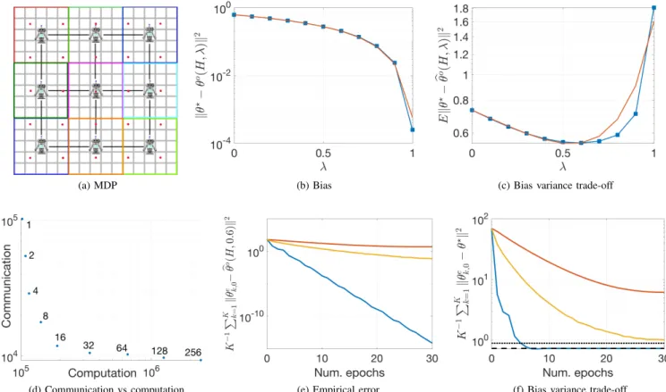
The MDP’s specifications are as follows. The state space is given by a 15×15 grid and the possible actions are: UP, DOWN, LEFT and RIGHT. The reward structure of the MDP and the target policy were generated randomly. We consider a network of9agents that divide the state space in 9 regions. The topology of the network and the regions assigned to the agents for exploration are shown in Figure 1a. The feature vectors consist of 26 features, 25 given by radial basis functions3 (RBF) centered in the red marks show in Figure 1a plus one 2Note that in this case if sampling weights were to be used for off-policy
operation, every agent would require knowledge of the teams behavior policy.
3Each RBF is given byexp 0.5 (x−x
c)2+(y−yc)2, wherexcandyc
are the coordinates of the center of that feature andxandyare the coordinates of the agent.
bias feature fixed at+1. The behavior policy of every agent is equal to the target policy, except in the edges of its exploration region, where the probabilities of the actions that would take the agent beyond its exploration region are zeroed (the policy is further re-normalized).
In this experiment we show the bias-variance trade-off han-dled by the eligibility trace parameterλ, the communication-computation trade-off handled by the mini-batch size, and the performance ofFDPEcompared to the existing algorithms that can be applied to this scenario (namely Diffusion GTD2 and ALG2). The hyper-parameters chosen forFDPEareτk= 1/9, H= 20,η= 0andNk= 215+H−1.
In figures 1b and 1c we show the bias and bias+variance curves as functions ofλand its approximations using lemmas 1 and 2, respectively4. Note that the expressions provided in Lemmas 1 and 2 accurately capture the dependence of the bias and variance as functions of λ. The bias curve was calculated using (5) and (16). To estimate the combined effects of the bias and variance we calculatedkθbo(H,λ)−θ?k2(using expressions (22)) 20 times with independently generated data and averaged the results. Note that the obtained curves agree with our previous discussion on the effect of the parameterλ. In this experiment, the optimal value is approximatelyλ= 0.6. Figure 1d shows how communication and computation can be traded through the use of the mini-batch size. To obtain this figure, we fixed λ= 0.6 and run FDPE until an error smaller than10−10was obtained for the different batch sizes.
For each case, the step-sizes were adjusted to maximize performance for a fair comparison. Note that all points are Pareto optimal, and hence the optimal choice of mini-batch size depends on every particular implementation. The y-axis displays the amount of communication rounds that took place over the entire optimization process, while the x-axis shows the amount of sample gradients calculated. Figure 1e shows the empirical squared error for the three algorithms (each curve was obtained by averaging the squared errors from all the agents), where clearly the linear convergence of our algorithm can be seen. Finally, Figure 1f shows the mean square deviation (MSD), i.e., kθe
k,0−θ ?
k2. As can be seen,
our algorithm still outperforms the other algorithms in terms of convergence speed. It also has the advantage that it converges to a lower error (the dashed line) versus the other algorithms which converge to the dotted line, although in this case since the variance is high this advantage is not very significant. Note that as more data becomes available the variance of b
θo(H,λ) becomes smaller (see Lemma 2) and hence the
advantages (in terms of convergence speed and the minimizer that the algorithms converges to) of usingFDPEover the other algorithms becomes more pronounced. The remaining hyper-parameters for FDPE were: τk= 1/9, J= 210 (i.e., batch size equal to 32),µθ= 10andµω= 16. ForDiffusion GTD2 and ALG2 decaying step-sizes were employed to guarantee convergence. The step-sizes decayed asµ(1+0.01e)−1, where eis the epoch number (we used this decaying rule because it provided the best results). The initial step-sizes wereµθ= 1.1
and µω= 1.7 for Diffusion GTD2, and µθ= 2.5 and µω= 4
4The constantsκ
(a) MDP (b) Bias (c) Bias variance trade-off
(d) Communication vs computation (e) Empirical error (f) Bias variance trade-off
Fig. 1: In (b) and (c) the red curves are the approximations from lemmas 1 and 2. In (e) and (f), the blue curve corresponds toFDPEand red and yellow correspond toDiffusion GTD2 andALG2, respectively. In (f) the dotted line is at
kθb(H,λ= 0)−θ?k2 while the dashed line is at kθb(H,λ= 0.6)−θ?k2.
for ALG2.
B. Experiment II
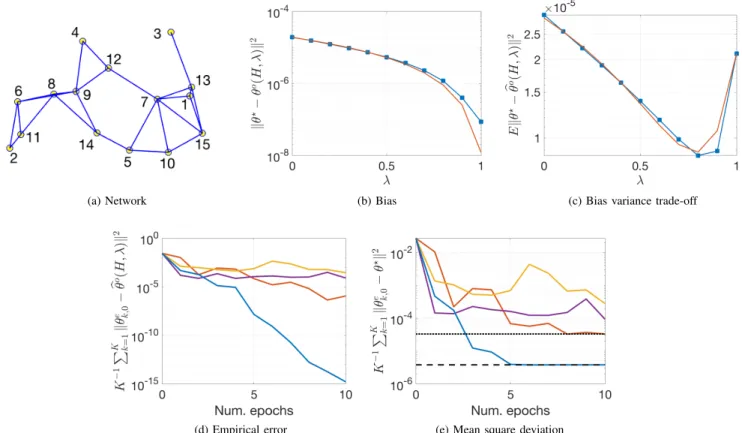
The second experiment relates to the MARL scenario of section IV. Similarly to [39], we consider randomly generated MDP’s. We consider a random network of K= 15agents. To construct the network, K agents are randomly distributed in a unit square (using a uniform distribution) and agents that are within a distance smaller thanr= 0.27become neighbors, which results in a sparsely connected network. The resulting network is shown in Figure 2a. The combination weights are determined according to the Metropolis rule which is given by: `nk= 1 max[|Nn|,|Nk|] n∈ Nk\{k} 1− P m∈Nk\{k} `mk n=k (69)
The generated MDP’s have 50 states and 10 actions. The transition probabilitiesp(s0|s,a)are zero with 0.98 probability and otherwise are sampled from a uniform distribution from the interval [0,1]. The probabilities are further normalized. With this sampling strategy, we produce realistic MDPs in which from any given state it is only possible to transition to a small subset of the total states. The rewards r(s0|s,a) are zero with 0.99 probability and otherwise are sampled from a Gaussian distribution with zero mean and standard
deviation equal to 10. This sampling strategy is also devised to produce more realistic MDPs where rewards are obtained occasionally in specific state-action pairs. The entries of the target policyπ(a|s) are sampled from a uniform distribution and subsequently normalized. The transition probabilities and target policy are sampled until Assumption 1 is satisfied. We set the discount factor γ= 0.93 and the length of the feature vectors M= 5, where one feature is set to 1 and the remaining ones are sampled from a uniform distribution with interval [0,1]. We generated N= 218+H
−1 team transitions. The remaining parameters for the learning algorithm are the following:H= 20,η= 10−3,U=I,θ
p=θo(H,λ)+θn(where
θnis a noise vector whose entries are sampled from a uniform distribution with variance equal to2.5×10−5) andτk= 1/15.
We compare our algorithm with PD-distIAG from [18], Diffusion GTD2andALG2. In this experiment, we test the on-policy case becausePD-distIAGonly works for this scenario. In Figures 2b and 2c, we show the bias variance trade-off as a function of λ (the curves were obtained in the same manner as done in the previous experiment). Results are consistent with the ones obtained in the previous section. In this particular case the most convenient value is approximately
λ= 0.8. In Figure 2d we compare the convergence rates of the different algorithms to solve the empirical problem. The hyper-parameters of all algorithms were tunned to maximize performance. The parameters for FDPE were: J= 212 (i.e.,
(a) Network (b) Bias (c) Bias variance trade-off
(d) Empirical error (e) Mean square deviation
Fig. 2: In (b), (c) and (d) the red curves are the approximations from lemmas 1 and 2. In (e) the blue, purple, yellow and red curves correspond to FDPE,Diffusion GTD2,ALG2andPD-distIAG, respectively. In (d) the dotted line is at
kθb(H,λ= 0)−θ?
k2 while the dashed line is at
kθb(H,λ= 0.6)−θ?
k2.
batch size equal to64),µθ= 10andµω= 10. ForPD-distIAG
we used the same batch size, and the step-sizes wereµθ= 1.15
and µω= 23. For Diffusion GTD2 andALG2 decaying
step-sizes were employed to guarantee convergence. The step-step-sizes decayed asµ(1+0.01e)−1, whereeis the epoch number (we
used this decaying rule because it provided the best results). The initial step-sizes wereµθ= 15andµω= 7.5forDiffusion GTD2, and the same values for ALG2. In this experiment FDPE,Diffusion GTD2 and ALG2show performance in ac-cordance to our theory and the results in the previous section. PD-distIAGshows a linear convergence rate in accordance to the theory from [18]. However, the rate is slower than the one from our algorithm. Finally, in Figure 2e we show the MSD. Again, the faster convergence of our algorithm to its empirical minimizer implies a faster convergence in the MSD plot. In this case, the advantage of the parameter λ becomes more noticeable. Note indeed that the minimizer obtained by FDPE is approximately one order of magnitude smaller than the minimizer to which the other algorithms will converge (the dotted line).
APPENDIXA PROOF OFLEMMA1
To simplify the notation we refer to θo(H,λ)as θo. Using (16) and defining R=A−1CA−TU, we can write θo= (I+
ηR)−1(ηRθ
p+A−1b). Using the Jordan decomposition R=
JRΛRJR−1 we get:
θo= (I+ηR)−1A−1b+ηJR(I+ηΛR)−1ΛRJR−1θp (70) Note thatθocan be approximated by the following expression,
which has the advantage that it separates the effect of the regularization term on the bias:
θo= (I+κ1η)−1A−1b+κ1η(1+κ1η)−1θp (71) We proceed to calculate the bias ofθ•=A−1bwith respect to θ?. Using (7) and (12) we can write:
vπ= Γ2rπ+ρ1Γ1vπ= ∞ X n=0 (ρ1Γ1)nΓ2rπ (72) Xθ•= Π(Γ2rπ+ρ1Γ1Xθ•) = Π ∞ X n=0 (ρ1Γ1Π)nΓ2rπ (73) Xθ?= Πvπ= Π ∞ X n=0 (ρ1Γ1)nΓ2rπ (74)
Combining the expressions from above we get:
X(θ•−θ?) = Π ∞ X n=0 (ρ1Γ1Π)nΓ2rπ−vπ (75) = Π ∞ X n=1 (ρ1Γ1Π)n−(ρ1Γ1)n Γ2rπ (76)
Note that if vπ= Πvπ=Xθ?, then (72) can be rewritten as: vπ= ∞ X n=0 (ρ1Γ1Π)nΓ2rπ (77)
Combining (77) with (75) we get that if vπ= Πvπ, then θˇ−
θ?= 0. Therefore, we can write (76) as: X(θ•−θ?) =I(vπ6= Πvπ)Π ∞ X n=1 ρn1 (Γ1Π)n−Γn1 Γ2rπ (78)
where I is the indicator function. We now approximate the right stochastic matrix Pπ by it’s steady state limit (given
by (Pπ)∞=
1pT, where
1 is the all ones vector and p is the vector with the steady state distribution induced by the transition matrixPπ). Consequently, we get:
Γ1≈1pT (79) Γ2rπ≈ 1−(γλ)H 1−γλ 1p Trπ= 1 −ρ1 1−γ 1pTrπ (80) =pTΠ1 (81) ∞ X n=1 ρn1((Γ1Π)n−Γn1)Γ2rπ≈ ∞ X n=1 ρn1 (1pTΠ)n−1pTΓ2rπ (82) =1 1 −(γλ)H 1−γλ pTrπ ∞ X n=1 ρn1( n −1) (83) Since pT1= 1andΠis a projection matrix (and therefore its eigenvalues are either0or1) we get that|| ≤1and therefore we can write: ∞ X n=1 ρn1(n−1) = ρ1 1−ρ1− ρ1 1−ρ1 = ρ1(−1) (1−ρ1)(1−ρ1) (84) ∞ X n=1 ρn1((Γ1Π)n−Γn1)Γ2rπ≈1pTrπ=O ρ 1(−1) (1−ρ1)(1−γ) (85) Therefore, combining (71), (78) and (85) and grouping con-stants we can finally write:
kθo−θ?k2≈ I vπ6=Πvπ κ2ρ1 (1+κ1η)(κ3−ρ1) +κ1ηkθp−θ ? k 1+κ1η 2 (86) APPENDIXB PROOF OFLEMMA2
Since the regularization term of (71) is not subject to variance, to calculate the variance in the estimate of θbo we
need to calculate the variance of θb•=Ab−1ˆb as follows:
Ekθb•−θ• k2=E kAb−1ˆb−θ•k2=E bA−1 ˆb−Aθb • 2 (87) where we are using the squared Euclidean norm. Due to the Rayleigh-Ritz’ Theorem we have σmin(Ab−1)≤ kAb−1k ≤
σmax(Ab−1)and sinceσmax(Ab) =σmin(Ab−1)andσmax(Ab−1) =
σmin(Ab)we can write:
Ekθb•−θ• k2 ≤Eσmin2 (Ab)ˆb−Aθb • 2 (88) Ekθb•−θ• k2 ≥Eσmax2 (Ab) ˆb−Aθb • 2 (89)
Now using Proposition 9.6.8 of [40] and the fact that Ab= b
C−XTDΓb
1X we can write:
σmin(Ab) =λmin(Cb)±ρ1σmax(Eb) =λmin(Cb)+O(ρ1) (90) σmax(Ab) =λmax(Cb)±ρ1σmax(Eb) =λmax(Cb)+O(ρ1) (91)
b
E=XTDΓb1X (92)
Using the above results and the intermediate value theorem we can write: Ekθb•−θ• k2= ( 2+O(ρ1)) 2ˆ b−Aθb •2 (93) for some constant2. For E
ˆb−Aθb •2 we can write: Eˆb−Aθb •2 =E NX−H t=1 ˆb t−Abtθ• N−H 2 (b) =Ek ˆb t−Abtθ•k2 N−H (94)
where in(b)we assumed that the total amount of data collected is significantly larger than the mixing rate of the Markov Chain, and therefore the terms ˆbt−Atθb • corresponding to different times can be considered independent of each other. Note that this is a standard assumption (similar to the one stated in Assumption 4) in the sense that in practice it demands that enough data is gathered so that the effect of the policy on every state can be accurately estimated. To approximate
Eˆb t−Abtθ• 2 we proceed as follows: Eˆb t−Abtθ• 2 =Ekxtk2 (γλ)H−1(rt+H−1+γxTt+Hθ•) + HX−2 n=0 (γλ)n rt+n+γ(1−λ)xTt+n+1θ• −xTtθ• 2 (95) (a) =Ekxtk2 HX−1 n=0 (γλ)n xTt+nθ•−rt+n−γxTt+n+1θ• !2 (96) (b) ≈Ekxtk2 H−1 X n=0 (γλ)n(v(st+n)−rt+n−γv(st+n+1)) !2 (97) (c) =Ekxtk2 HX−1 n=0 (γλ)2n(v(st+n)−rt+n−γv(st+n+1)) 2 (98) where in (a) we simply reorganized the terms, in (b) we used xT
tθ•≈v(st) and in (c) we used the fact that
due to the Markov property each term v(st+n)−rt+n− γv(st+n+1) is conditionally independent from all
previ-ous terms (conditioned on st+n) and that by definition
E[v(st+n)−rt+n−γv(st+n+1)|st+n] = 0. Now we lower and
upper bound (98) as follows:
m HX−1 n=0 (γλ)2n≤Eˆbt−Abtθ• 2 ≤M HX−1 n=0 (γλ)2n (99) M= max t,n kxtk 2(v(st +n)−rt+n−γv(st+n+1))2 (100) m= min t,n kxtk 2(v(s t+n)−rt+n−γv(st+n+1)) 2 (101) Combining the above result with the intermediate value theo-rem we get: Eˆb t−Abtθ• 2 ≈3 1 −(γλ)2H 1−(γλ)2 (102)