Machine Learning and Data Mining Lecture Notes - Free Computer, Programming, Mathematics, Technical Books, Lecture Notes and Tutorials

(1)

Lecture Notes

CSC 411/D11

Computer Science Department

University of Toronto

Version: February 6, 2012

(2)

Conventions and Notation

Scalars are written with lower-case italics, e.g.,x. Column-vectors are written in bold, lower-case:

x, and matrices are written in bold uppercase:B.

The set of real numbers is represented by_R;N-dimensional Euclidean space is written_RN.

Aside:

Text in “aside” boxes provide extra background or information that you are not re-quired to know for this course.

Acknowledgements

(6)

1 Introduction to Machine Learning

Machine learning is a set of tools that, broadly speaking, allow us to “teach” computers how to perform tasks by providing examples of how they should be done. For example, suppose we wish to write a program to distinguish between valid email messages and unwanted spam. We could try to write a set of simple rules, for example, flagging messages that contain certain features (such as the word “viagra” or obviously-fake headers). However, writing rules to accurately distinguish which text is valid can actually be quite difficult to do well, resulting either in many missed spam messages, or, worse, many lost emails. Worse, the spammers will actively adjust the way they send spam in order to trick these strategies (e.g., writing “vi@gr@”). Writing effective rules — and keeping them up-to-date — quickly becomes an insurmountable task. Fortunately, machine learning has provided a solution. Modern spam filters are “learned” from examples: we provide the learning algorithm with example emails which we have manually labeled as “ham” (valid email) or “spam” (unwanted email), and the algorithms learn to distinguish between them automatically.

Machine learning is a diverse and exciting field, and there are multiple ways of defining it:

1. The Artifical Intelligence View. Learning is central to human knowledge and intelligence, and, likewise, it is also essential for building intelligent machines. Years of effort in AI has shown that trying to build intelligent computers by programming all the rules cannot be done; automatic learning is crucial. For example, we humans are not born with the ability to understand language — we learn it — and it makes sense to try to have computers learn language instead of trying to program it all it.

2. The Software Engineering View. Machine learning allows us to program computers by example, which can be easier than writing code the traditional way.

3. The Stats View. Machine learning is the marriage of computer science and statistics: com-putational techniques are applied to statistical problems. Machine learning has been applied to a vast number of problems in many contexts, beyond the typical statistics problems. Ma-chine learning is often designed with different considerations than statistics (e.g., speed is often more important than accuracy).

Often, machine learning methods are broken into two phases:

1. Training: A model is learned from a collection of training data.

2. Application: The model is used to make decisions about some new test data.

(7)

1.1 Types of Machine Learning

Some of the main types of machine learning are:

1. Supervised Learning, in which the training data is labeled with the correct answers, e.g., “spam” or “ham.” The two most common types of supervised learning are classification (where the outputs are discrete labels, as in spam filtering) and regression (where the outputs are real-valued).

2. Unsupervised learning, in which we are given a collection of unlabeled data, which we wish to analyze and discover patterns within. The two most important examples are dimension reduction and clustering.

3. Reinforcement learning, in which an agent (e.g., a robot or controller) seeks to learn the optimal actions to take based the outcomes of past actions.

There are many other types of machine learning as well, for example:

1. Semi-supervised learning, in which only a subset of the training data is labeled

2. Time-series forecasting, such as in financial markets

3. Anomaly detection such as used for fault-detection in factories and in surveillance

4. Active learning, in which obtaining data is expensive, and so an algorithm must determine which training data to acquire

and many others.

1.2 A simple problem

Figure 1 shows a 1D regression problem. The goal is to fit a 1D curve to a few points. Which curve is best to fit these points? There are infinitely many curves that fit the data, and, because the data might be noisy, we might not even want to fit the data precisely. Hence, machine learning requires that we make certain choices:

1. How do we parameterize the model we fit? For the example in Figure 1, how do we param-eterize the curve; should we try to explain the data with a linear function, a quadratic, or a sinusoidal curve?

(8)

3. Some types of models and some model parameters can be very expensive to optimize well. How long are we willing to wait for a solution, or can we use approximations (or hand-tuning) instead?

4. Ideally we want to find a model that will provide useful predictions in future situations. That is, although we might learn a model from training data, we ultimately care about how well it works on future test data. When a model fits training data well, but performs poorly on test data, we say that the model has overfit the training data; i.e., the model has fit properties of the input that are not particularly relevant to the task at hand (e.g., Figures 1 (top row and bottom left)). Such properties are refered to as noise. When this happens we say that the model does not generalize well to the test data. Rather it produces predictions on the test data that are much less accurate than you might have hoped for given the fit to the training data.

(9)

0 1 2 3 4 5 6 7 8 9 10 −1.5

−1 −0.5 0 0.5 1 1.5

0 1 2 3 4 5 6 7 8 9 10

−1.5 −1 −0.5 0 0.5 1 1.5

0 1 2 3 4 5 6 7 8 9 10

−6 −4 −2 0 2 4 6

0 1 2 3 4 5 6 7 8 9 10

−1 −0.5 0 0.5 1 1.5

(10)

2 Linear Regression

In regression, our goal is to learn a mapping from one real-valued space to another. Linear re-gression is the simplest form of rere-gression: it is easy to understand, often quite effective, and very efficient to learn and use.

2.1 The 1D case

We will start by considering linear regression in just 1 dimension. Here, our goal is to learn a mappingy =f(x), wherexandyare both real-valued scalars (i.e.,x _∈_R, y _∈ _R). We will take

f to be an linear function of the form:

y=wx+b (1)

where w is a weight and b is a bias. These two scalars are the parameters of the model, which we would like to learn from training data. n particular, we wish to estimate wand bfrom the N

training pairs _{(xi, yi)}Ni=1. Then, once we have values forw andb, we can compute the y for a

newx.

Given 2 data points (i.e., N=2), we can exactly solve for the unknown slope w and offset b. (How would you formulate this solution?) Unfortunately, this approach is extremely sensitive to noise in the training data measurements, so you cannot usually trust the resulting model. Instead, we can find much better models when the two parameters are estimated from larger data sets. WhenN > 2we will not be able to find unique parameter values for whichyi = wxi+bfor all

i, since we have many more constraints than parameters. The best we can hope for is to find the parameters that minimize the residual errors, i.e.,yi−(wxi +b).

The most commonly-used way to estimate the parameters is by least-squares regression. We define an energy function (a.k.a. objective function):

E(w, b) =

N

X

i=1

(yi−(wxi +b))2 (2)

To estimate wandb, we solve for thew andbthat minimize this objective function. This can be done by setting the derivatives to zero and solving.

dE

db = −2

X

i

(yi−(wxi+b)) = 0 (3)

Solving forbgives us the estimate:

b∗ =

P

iyi

N −w

P

ixi

N (4)

(11)

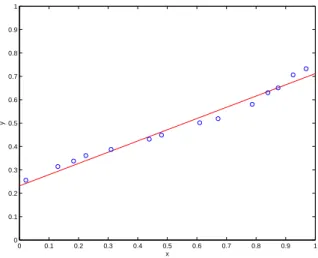
0 0.1 0.2 0.3 0.4 0.5 0.6 0.7 0.8 0.9 1 0

0.1 0.2 0.3 0.4 0.5 0.6 0.7 0.8 0.9 1

x

y

Figure 2: An example of linear regression: the red line is fit to the blue data points.

where we definex¯andy¯as the averages of thex’s andy’s, respectively. This equation for b∗ _still

depends onw, but we can nevertheless substitute it back into the energy function:

E(w, b) = X

i

((yi−y¯)−w(xi−x¯))2 (6)

Then:

dE

dw = −2

X

i

((yi−y¯)−w(xi−x¯))(xi−x¯) (7)

Solving dE_dw = 0then gives:

w∗ =

P

i(yi−y¯)(xi−x¯)

P

i(xi−x¯)2

(8)

The valuesw∗ _and_b∗_{are the least-squares estimates for the parameters of the linear regression.}

2.2 Multidimensional inputs

Now, suppose we wish to learn a mapping fromD-dimensional inputs to scalar outputs: x_∈_RD,

y_∈R. Now, we will learn a vector of weightsw, so that the mapping will be:1

f(x) =wTx+b=

D

X

j=1

wjxj +b . (9)

1_{Above we used subscripts to index the training set, while here we are using the subscript to index the elements of}

(12)

For convenience, we can fold the bias binto the weights, if we augment the inputs with an addi-tional 1. In other words, if we define

˜ w=      w1 .. . wD b     

, x˜=

     x1 .. . xD 1      (10)

then the mapping can be written:

f(x) = ˜wTx˜. (11)

GivenN training input-output pairs, the least-squares objective function is then:

E( ˜w) =

N

X

i=1

(yi−w˜Tx˜i)2 (12)

If we stack the outputs in a vector and the inputs in a matrix, then we can also write this as:

E( ˜w) =||y₋X˜w˜_||2 (13) where y=    y1 .. . yN  

, X˜ = 

 

xT₁ 1

.. .

xT_N 1





 (14)

and _{|| · ||}is the usual Euclidean norm, i.e., _||v_||2 = P_iv2

i. (You should verify for yourself that

Equations 12 and 13 are equivalent).

Equation 13 is known as a linear least-squares problem, and can be solved by methods from linear algebra. We can rewrite the objective function as:

E(w) = (y₋X˜w˜)T(y₋X˜w˜) (15) = w˜TX˜TX˜w˜ ₋2yTX˜w˜ +yTy (16)

We can optimize this by setting all values of dE/dwi = 0 and solving the resulting system of

equations (we will cover this in more detail later in Chapter 4). In the meantime, if this is unclear, start by reviewing your linear algebra and vector calculus). The solution is given by:

w∗ = ( ˜XTX˜)−1X˜Ty (17) (You may wish to verify for yourself that this reduces to the solution for the 1D case in Section 2.1; however, this takes quite a lot of linear algebra and a little cleverness). The matrix X˜+ _≡

( ˜XTX˜)−1_X_˜T _{is called the pseudoinverse of}_X_˜_{, and so the solution can also be written:}

˜

(13)

In MATLAB, one can directly solve the system of equations using the slash operator:

˜

w∗ = ˜X\y (19)

There are some subtle differences between these two ways of solving the system of equations. We will not concern ourselves with these here except to say that I recommend using the slash operator rather than the pseudoinverse.

2.3 Multidimensional outputs

In the most general case, both the inputs and outputs may be multidimensional. For example, with

D-dimensional inputs, andK-dimensional outputsy_∈_RK, a linear mapping from input to output can be written as

y= ˜WTx˜ (20)

whereW˜ _∈_R(D+1)×K. It is convenient to expressW˜ in terms of its column vectors, i.e., ˜

W= [ ˜w1 . . . w˜K]≡

w1 . . . wK

b1 . . . bK

. (21)

In this way we can then express the mapping from the inputx˜to thejthelement ofyasyj = ˜wTjx.

Now, givenN training samples, denoted_{x˜_i,y_i_}N

i=1a natural energy function to minimize in order

to estimateW˜ is just the squared residual error over all training samples and all output dimensions, i.e.,

E( ˜W) =

N

X

i=1

K

X

j=1

(yi,j −w˜Tjx˜i)2. (22)

There are several ways to conveniently vectorize this energy function. One way is to express

Esolely as a sum over output dimensions. That is, lety′_j be theN-dimensional vector comprising thejth_{component of each output training vector, i.e.,}_y′

j = [y1,j, y2,j, ..., yN,j]T. Then we can write

E( ˜W) =

K

X

j=1

||y′_j ₋X˜w˜_j_||2 (23)

where X˜T = [˜x1x˜2 . . . x˜N]. With a little thought you can see that this really amounts to K

distinct estimation problems, the solutions for which are given byw˜∗_j = ˜X+y′_j. Another common convention is to stack up everything into a matrix equation, i.e.,

E( ˜W) =_||Y₋X˜W˜ _||2_F (24) whereY = [y′₁ . . .y′_K], and_{|| · ||}F denotes the Frobenius norm: ||Y||2F =

P

i,jY2i,j. You should

verify that Equations (23) and (24) are equivalent representations of the energy function in Equa-tion (22). Finally, the soluEqua-tion is again provided by the pseudoinverse:

˜

W∗ = ˜X+Y (25)

(14)

3 Nonlinear Regression

Sometimes linear models are not sufficient to capture the real-world phenomena, and thus nonlinear models are necessary. In regression, all such models will have the same basic form, i.e.,

y=f(x) (26)

In linear regression, we havef(x) = Wx+b; the parametersWandbmust be fit to data. What nonlinear function do we choose? In principle,f(x)could be anything: it could involve linear functions, sines and cosines, summations, and so on. However, the form we choose will make a big difference on the effectiveness of the regression: a more general model will require more data to fit, and different models are more appropriate for different problems. Ideally, the form of the model would be matched exactly to the underlying phenomenon. If we’re modeling a linear process, we’d use a linear regression; if we were modeling a physical process, we could, in principle, modelf(x)by the equations of physics.

In many situations, we do not know much about the underlying nature of the process being modeled, or else modeling it precisely is too difficult. In these cases, we typically turn to a few models in machine learning that are widely-used and quite effective for many problems. These methods include basis function regression (including Radial Basis Functions), Artificial Neural Networks, andk-Nearest Neighbors.

There is one other important choice to be made, namely, the choice of objective function for learning, or, equivalently, the underlying noise model. In this section we extend the LS estimators introduced in the previous chapter to include one or more terms to encourage smoothness in the estimated models. It is hoped that smoother models will tend to overfit the training data less and therefore generalize somewhat better.

3.1 Basis function regression

A common choice for the functionf(x)is a basis function representation2_:

y=f(x) =X

k

wkbk(x) (27)

for the 1D case. The functions bk(x) are called basis functions. Often it will be convenient to

express this model in vector form, for which we define b(x) = [b1(x), . . . , bM(x)]T and w =

[w1, . . . , wM]T whereM is the number of basis functions. We can then rewrite the model as

y=f(x) = b(x)Tw (28)

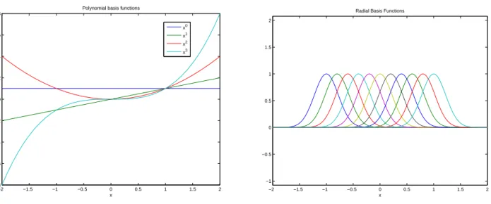
Two common choices of basis functions are polynomials and Radial Basis Functions (RBF). A simple, common basis for polynomials are the monomials, i.e.,

b0(x) = 1, b1(x) =x, b2(x) = x2, b3(x) =x3, ... (29)

2_{In the machine learning and statistics literature, these representations are often referred to as linear regression,}

(15)

−2 −1.5 −1 −0.5 0 0.5 1 1.5 2 −8

−6 −4 −2 0 2 4 6 8

x Polynomial basis functions

x0 x1

x2 x3

−2 −1.5 −1 −0.5 0 0.5 1 1.5 2 −1

−0.5 0 0.5 1 1.5 2

x Radial Basis Functions

Figure 3: The first three basis functions of a polynomial basis, and Radial Basis Functions

With a monomial basis, the regression model has the form

f(x) = Xwkxk, (30)

Radial Basis Functions, and the resulting regression model are given by

bk(x) = e−

(x−_ck)2

2σ2 , (31) f(x) = Xwke−

(x−_ck)2

2σ2 , (32)

whereck is the center (i.e., the location) of the basis function andσ2 determines the width of the

basis function. Both of these are parameters of the model that must be determined somehow. In practice there are many other possible choices for basis functions, including sinusoidal func-tions, and other types of polynomials. Also, basis functions from different families, such as mono-mials and RBFs, can be combined. We might, for example, form a basis using the first few poly-nomials and a collection of RBFs. In general we ideally want to choose a family of basis functions such that we get a good fit to the data with a small basis set so that the number of weights to be estimated is not too large.

To fit these models, we can again use least-squares regression, by minimizing the sum of squared residual error between model predictions and the training data outputs:

E(w) = X

i

(yi−f(xi))2 =

X

i

yi−

X

k

wkbk(x)

!2

(33)

(16)

In particular, E is still quadratic in the weightsw, and hence the weightswcan be estimated the same way. That is, we can rewrite the objective function in matrix-vector form to produce

E(w) = _||y₋Bw_||2 (34) where_||·||denotes the Euclidean norm, and the elements of the matrixBare given byB_i,j =bj(xi)

(for rowiand columnj). In Matlab the least-squares estimate can be computed asw∗ =B\y.

Picking the other parameters. The positions of the centers and the widths of the RBF basis functions cannot be solved directly for in closed form. So we need some other criteria to select them. If we optimize these parameters for the squared-error, then we will end up with one basis center at each data point, and with tiny width that exactly fit the data. This is a problem as such a model will not usually provide good predictions for inputs other than those in the training set.

The following heuristics instead are commonly used to determine these parameters without overfitting the training data. To pick the basis centers:

1. Place the centers uniformly spaced in the region containing the data. This is quite simple, but can lead to empty regions with basis functions, and will have an impractical number of data points in higher-dimensinal input spaces.

2. Place one center at each data point. This is used more often, since it limits the number of centers needed, although it can also be expensive if the number of data points is large.

3. Cluster the data, and use one center for each cluster. We will cover clustering methods later in the course.

To pick the width parameter:

1. Manually try different values of the width and pick the best by trial-and-error.

2. Use the average squared distances (or median distances) to neighboring centers, scaled by a constant, to be the width. This approach also allows you to use different widths for different basis functions, and it allows the basis functions to be spaced non-uniformly.

In later chapters we will discuss other methods for determining these and other parameters of models.

3.2 Overfitting and Regularization

(17)

1. The problem is insufficiently constrained: for example, if we have ten measurements and ten model parameters, then we can often obtain a perfect fit to the data.

2. Fitting noise: overfitting can occur when the model is so powerful that it can fit the data and also the random noise in the data.

3. Discarding uncertainty: the posterior probability distribution of the unknowns is insuffi-ciently peaked to pick a single estimate. (We will explain what this means in more detail later.)

There are two important solutions to the overfitting problem: adding prior knowledge and handling uncertainty. The latter one we will discuss later in the course.

In many cases, there is some sort of prior knowledge we can leverage. A very common as-sumption is that the underlying function is likely to be smooth, for example, having small deriva-tives. Smoothness distinguishes the examples in Figure 4. There is also a practical reason to prefer smoothness, in that assuming smoothness reduces model complexity: it is easier to estimate smooth models from small datasets. In the extreme, if we make no prior assumptions about the nature of the fit then it is impossible to learn and generalize at all; smoothness assumptions are one way of constraining the space of models so that we have any hope of learning from small datasets. One way to add smoothness is to parameterize the model in a smooth way (e.g., making the width parameter for RBFs larger; using only low-order polynomial basis functions), but this limits the expressiveness of the model. In particular, when we have lots and lots of data, we would like the data to be able to “overrule” the smoothness assumptions. With large widths, it is impossible to get highly-curved models no matter what the data says.

Instead, we can add regularization: an extra term to the learning objective function that prefers smooth models. For example, for RBF regression with scalar outputs, and with many other types of basis functions or multi-dimensional outputs, this can be done with an objective function of the form:

E(w) =||y₋Bw_||2

| {z }

data term

+ λ||w_||2 | {z }

smoothness term

(35)

This objective function has two terms. The first term, called the data term, measures the model fit to the training data. The second term, often called the smoothness term, penalizes non-smoothness (rapid changes inf(x)). This particular smoothness term (_||w_||) is called weight decay, because it tends to make the weights smaller.3 _{Weight decay implicitly leads to smoothness with RBF basis}

functions because the basis functions themselves are smooth, so rapid changes in the slope off

(i.e., high curvature) can only be created in RBFs by adding and subtracting basis functions with large weights. (Ideally, we might directly penalize smoothness, e.g., using an objective term that directly penalizes the integral of the squared curvature off(x), but this is usually impractical.)

(18)

This regularized least-squares objective function is still quadratic with respect towand can be optimized in closed-form. To see this, we can rewrite it as follows:

E(w) = (y₋Bw)T(y₋Bw) +λwTw (36) = wTBTBw₋2wTBTy+λwTw+yTy (37) = wT(BTB+λI)w₋2wTBTy+yTy (38)

To minimizeE(w), as above, we solve the normal equations_∇E(w) = 0(i.e., ∂E/∂wi = 0for

alli). This yields the following regularized LS estimate forw:

w∗ = (BTB+λI)−1BTy (39)

3.3 Artificial Neural Networks

Another choice of basis function is the sigmoid function. “Sigmoid” literally means “s-shaped.” The most common choice of sigmoid is:

g(a) = 1

1 +e−a (40)

Sigmoids can be combined to create a model called an Artificial Neural Network (ANN). For regression with multi-dimensional inputsx_∈_RK₂ , and multidimensional outputsy_∈_RK1_:

y=f(x) =X

j

w(1)_j g X

k

w(2)_k,jxk+b(2)j

!

+b(1) (41)

This equation describes a process whereby a linear regressor with weights w(2)is applied to x. The output of this regressor is then put through the nonlinear Sigmoid function, the outputs of which act as features to another linear regressor. Thus, note that the inner weightsw(2)_{are distinct}

parameters from the outer weights w(1)_j . As usual, it is easiest to interpret this model in the 1D case, i.e.,

y =f(x) =X

j

w(1)_j gw_j(2)x+b(2)_j +b(1) (42)

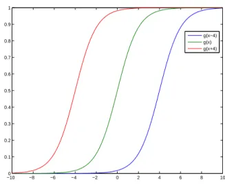
Figure 5(left) shows plots ofg(wx)for different values ofw, and Figure 5(right) showsg(x+b) for different values of b. As can be seen from the figures, the sigmoid function acts more or less like a step function for large values ofw, and more like a linear ramp for small values ofw. The biasbshifts the function left or right. Hence, the neural network is a linear combination of shifted (smoothed) step functions, linear ramps, and the bias term.

To learn an artificial neural network, we can again write a regularized squared-error objective function:

(19)

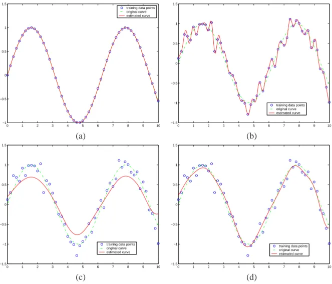
0 1 2 3 4 5 6 7 8 9 10 −1

−0.5 0 0.5 1 1.5

training data points original curve estimated curve

0 1 2 3 4 5 6 7 8 9 10

−1.5 −1 −0.5 0 0.5 1 1.5

(a) (b)

0 1 2 3 4 5 6 7 8 9 10

−1.5 −1 −0.5 0 0.5 1 1.5

0 1 2 3 4 5 6 7 8 9 10

−1.5 −1 −0.5 0 0.5 1 1.5

(c) (d)

(20)

−100 −8 −6 −4 −2 0 2 4 6 8 10 0.1

0.2 0.3 0.4 0.5 0.6 0.7 0.8 0.9 1

g(x−4) g(x) g(x+4)

Figure 5: Left: Sigmoidsg(wx) = 1/(1+e−wx₎_{for various values of}_w_{, ranging from linear ramps}

to smooth steps to nearly hard steps. Right: Sigmoids g(x+b) = 1/(1 +e−x−b₎_{with different}

shiftsb.

wherewcomprises the weights at both levels for allj. Note that we regularize by applying weight decay to the weights (both inner and outer), but not the biases, since only the weights affect the smoothness of the resulting function (why?).

Unfortuntely, this objective function cannot be optimized in closed-form, and numerical opti-mization procedures must be used. We will study one such method, gradient descent, in the next chapter.

3.4 K

-Nearest Neighbors

At heart, many learning procedures — especially when our prior knowledge is weak — amount to smoothing the training data. RBF fitting is an example of this. However, many of these fitting procedures require making a number of decisions, such as the locations of the basis functions, and can be sensitive to these choices. This raises the question: why not cut out the middleman, and smooth the data directly? This is the idea behindK-Nearest Neighbors regression.

(21)

for those nearest neigbors. This can be expressed as:

y= 1

K

X

i∈NK(x)

yi (44)

where the setNK(x)contains the indicies of theK training points closest tox. Alternatively, we

might take a weighted average of theK-nearest neighbors to give more influence to training points close toxthan to those further away:

y=

P

i∈NK(x)w(xi)yi

P

i∈NK(x)w(xi)

, w(xi) =e−||xi−x||

2_/₂_σ2

(45)

whereσ2 _{is an additional parameter to the algorithm. The parameters}_K _and_σ_{control the degree}

of smoothing performed by the algorithm. In the extreme case ofK = 1, the algorithm produces a piecewise-constant function.

(22)

4 Quadratics

The objective functions used in linear least-squares and regularized least-squares are multidimen-sional quadratics. We now analyze multidimenmultidimen-sional quadratics further. We will see many more uses of quadratics further in the course, particularly when dealing with Gaussian distributions.

The general form of a one-dimensional quadratic is given by:

f(x) =w2x2+w1x+w0 (46) This can also be written in a slightly different way (called standard form):

f(x) = a(x₋b)2+c (47) where a = w2, b = ₋w1/(2w2), c = w0 ₋w2

1/4w2. These two forms are equivalent, and it is

easy to go back and forth between them (e.g., given a, b, c, what are w0, w1, w2?). In the latter form, it is easy to visualize the shape of the curve: it is a bowl, with minimum (or maximum) at

b, and the “width” of the bowl is determined by the magnitude of a, the sign of atells us which direction the bowl points (apositive means a convex bowl,anegative means a concave bowl), and

ctells us how high or low the bowl goes (atx = b). We will now generalize these intuitions for higher-dimensional quadratics.

The general form for a 2D quadratic function is:

f(x1, x2) = w1,1x21+w1,2x1x2+w2,2x22+w1x1+w2x2+w0 (48)

and, for anN-D quadratic, it is:

f(x1, ...xN) =

X

1≤i≤N,1≤j≤N

wi,jxixj+

X

1≤i≤N

wixi+w0 (49)

Note that there are three sets of terms: the quadratic terms (Pwi,jxixj), the linear terms (

P

wixi)

and the constant term (w0).

Dealing with these summations is rather cumbersome. We can simplify things by using matrix-vector notation. Letxbe anN-dimensional column vector, writtenx= [x1, ...xN]T. Then we can

write a quadratic as:

f(x) = xTAx+bTx+c (50)

where

A =



 

w1,1 ... w1,N

..

. wi,j ...

wN,1 ... wN,N





 (51)

b = [w1, ..., wN]T (52)

(23)

You should verify for yourself that these different forms are equivalent: by multiplying out all the elements off(x), either in the 2D case or, using summations, the generalN −Dcase.

For many manipulations we will want to do later, it is helpful for Ato be symmetric, i.e., to havewi,j =wj,i. In fact, it should be clear that these off-diagonal entries are redundant. So, if we

are a given a quadratic for whichAis asymmetric, we can symmetrize it as:

f(x) =xT(1

2(A+A

T₎₎_x₊_bT_x₊_c₌_xT_Ax_˜ ₊_bT_x₊_c ₍₅₄₎

and use A˜ = 1

2(A+A

T₎_{instead. You should confirm for yourself that this is equivalent to the}

original quadratic.

As before, we can convert the quadratic to a form that leads to clearer interpretation:

f(x) = (x₋µ)TA(x₋µ) +d (55)

whereµ = −1

2A−1b, d = c−µTAµ, assuming thatA−1 exists. Note the similarity here to the

1-D case. As before, this function is a bowl-shape inN dimensions, with curvature specified by the matrixA, and with a single stationary pointµ.4 _{However, fully understanding the shape of}

f(x)is a bit more subtle and interesting.

4.1 Optimizing a quadratic

Suppose we wish to find the stationary points (minima or maxima) of a quadratic

f(x) =xTAx+bTx+c. (56)

The stationary points occur where all partial derivatives are zero, i.e., ∂f /∂xi = 0 for alli. The

gradient of a function is the vector comprising the partial derivatives of the function, i.e.,

∇f _≡[∂f /∂x1, ∂f /∂x2, . . . , ∂f /∂N]T . (57)

At stationary points it must therefore be true that _∇f = [0, . . . ,0]T_{. Let us assume that} _A _is

symmetric (if it is not, then we can symmetrize it as above). Equation 56 is a very common form of cost function (e.g. the log probability of a Gaussian as we will later see), and so the form of its gradient is important to examine.

Due to the linearity of the differentiation operator, we can look at each of the three terms of Eq.56 separately. The last (constant) term does not depend onxand so we can ignore it because its derivative is zero. Let us examine the first term. If we write out the individual terms within the

(24)

vectors/matrices, we get:

(x1. . . xN)



 

a11 . . . a1N

..

. . .. ...

aN1 . . . aN N

      x1 .. . xN    (58)

= (x1a11+x2a21+. . .+xNaN1x1a12+x2a22+. . . (59)

. . .+x1a1N +x2a2N +. . .+xNaN N)

   x1 .. . xN    (60)

=x2₁a11+x1x2a21+. . .+x1xNaN1+x1x2a12+x22a22+. . .+xNx2aN2+. . . (61) . . . x1xNa1N +x2xNa2N +. . .+x2NaN N (62)

=X

ij

aijxixj (63)

The ith element of the gradient corresponds to ∂f /∂xi. So in the expression above, for the

terms in the gradient corresponding to eachxi, we only need to consider the terms involving xi

(others will have derivative zero), namely

x2_iaii+

X

j6=i

xixj(aij +aji) (64)

The gradient then has a very simple form:

∂ xTAx

∂xi

= 2xiaii+

X

j6=i

xj(aij +aji). (65)

We can write a single expression for all of thexiusing matrix/vector form:

∂xTAx

∂x = (A+A

T₎_x_. ₍₆₆₎

You should multiply this out for yourself to see that this corresponds to the individual terms above. If we assume thatAis symmetric, then we have

∂xTAx

∂x = 2Ax. (67)

This is also a very helpful rule that you should remember. The next term in the cost function,bTx, has an even simpler gradient. Note that this is simply a dot product, and the result is a scalar:

(25)

Only one term corresponds to each xi and so ∂f /∂xi = bi. We can again express this in

ma-trix/vector form:

∂ bTx

∂x =b. (69)

This is another helpful rule that you will encounter again. If we use both of the expressions we have just derived, and set the gradient of the cost function to zero, we get:

∂f(x)

∂x = 2Ax+b= [0, . . . ,0]

T ₍₇₀₎

The optimum is given by the solution to this system of equations (called normal equations):

x=₋1

2A

−1_b ₍₇₁₎

(26)

5 Basic Probability Theory

Probability theory addresses the following fundamental question: how do we reason? Reasoning is central to many areas of human endeavor, including philosophy (what is the best way to make decisions?), cognitive science (how does the mind work?), artificial intelligence (how do we build reasoning machines?), and science (how do we test and develop theories based on experimental data?). In nearly all real-world situations, our data and knowledge about the world is incomplete, indirect, and noisy; hence, uncertainty must be a fundamental part of our decision-making pro-cess. Bayesian reasoning provides a formal and consistent way to reasoning in the presence of uncertainty; probabilistic inference is an embodiment of common sense reasoning.

The approach we focus on here is Bayesian. Bayesian probability theory is distinguished by defining probabilities as degrees-of-belief. This is in contrast to Frequentist statistics, where the probability of an event is defined as its frequency in the limit of an infinite number of repeated trials.

5.1 Classical logic

Perhaps the most famous attempt to describe a formal system of reasoning is classical logic, origi-nally developed by Aristotle. In classical logic, we have some statements that may be true or false, and we have a set of rules which allow us to determine the truth or falsity of new statements. For example, suppose we introduce two statements, namedAandB:

A_≡“My car was stolen”

B_≡“My car is not in the parking spot where I remember leaving it”

Moreover, let us assert the rule “A impliesB”, which we will write as A _→ B. Then, ifA is known to be true, we may deduce logically that B must also be true (if my car is stolen then it won’t be in the parking spot where I left it). Alternatively, if I find my car where I left it (“B is false,” writtenB¯), then I may infer that it was not stolen (A¯) by the contrapositiveB¯ _→A¯.

Classical logic provides a model of how humans might reason, and a model of how we might build an “intelligent” computer. Unfortunately, classical logic has a significant shortcoming: it assumes that all knowledge is absolute. Logic requires that we know some facts about the world with absolute certainty, and then, we may deduce only those facts which must follow with absolute certainty.

In the real world, there are almost no facts that we know with absolute certainty — most of what we know about the world we acquire indirectly, through our five senses, or from dialogue with other people. One can therefore conclude that most of what we know about the world is uncertain. (Finding something that we know with certainty has occupied generations of philosophers.)

(27)

actual degree of plausibility depends on other contextual information — did I park it in a safe neighborhood?, did I park it in a handicapped zone?, etc.

Predicting the weather is another task that requires reasoning with uncertain information. While we can make some predictions with great confidence (e.g. we can reliably predict that it will not snow in June, north of the equator), we are often faced with much more difficult questions (will it rain today?) which we must infer from unreliable sources of information (e.g., the weather report, clouds in the sky, yesterday’s weather, etc.). In the end, we usually cannot determine for certain whether it will rain, but we do get a degree of certainty upon which to base decisions and decide whether or not to carry an umbrella.

Another important example of uncertain reasoning occurs whenever you meet someone new — at this time, you immediately make hundreds of inferences (mostly unconscious) about who this person is and what their emotions and goals are. You make these decisions based on the person’s appearance, the way they are dressed, their facial expressions, their actions, the context in which you meet, and what you have learned from previous experience with other people. Of course, you have no conclusive basis for forming opinions (e.g., the panhandler you meet on the street may be a method actor preparing for a role). However, we need to be able to make judgements about other people based on incomplete information; otherwise, normal interpersonal interaction would be impossible (e.g., how do you really know that everyone isn’t out to get you?).

What we need is a way of discussing not just true or false statements, but statements that have varying levels of certainty. In addition, we would like to be able to use our beliefs to reason about the world and interpret it. As we gain new information, our beliefs should change to reflect our greater knowledge. For example, for any two propositionsA andB(that may be true or false), if

A_→B, then strong belief inAshould increase our belief inB. Moreover, strong belief inBmay sometimes increase our belief inAas well.

5.2 Basic definitions and rules

The rules of probability theory provide a system for reasoning with uncertainty.There are a number of justifications for the use of probability theory to represent logic (such as Cox’s Axioms) that show, for certain particular definitions of common-sense reasoning, that probability theory is the only system that is consistent with common-sense reasoning. We will not cover these here (see, for example, Wikipedia for discussion of the Cox Axioms).

The basic rules of probability theory are as follows.

• The probability of a statement A — denoted P(A) — is a real number between 0 and 1, inclusive. P(A) = 1 indicates absolute certainty that A is true, P(A) = 0 indicates absolute certainty thatAis false, and values between 0 and 1 correspond to varying degrees of certainty.

(28)

• The conditional probability of A given B — denoted P(A_|B)— is the probability that we would assign to A being true, if we knewB to be true. The conditional probability is defined asP(A_|B) =P(A,B)/P(B).

• The Product Rule:

P(A,B) =P(A_|B)P(B) (72)

In other words, the probability thatAandBare both true is given by the probability thatBis true, multiplied by the probability we would assign toAif we knewBto be true. Similarly,

P(A,B) = P(B_|A)P(A). This rule follows directly from the definition of conditional probability.

• The Sum Rule:

P(A) +P( ¯A) = 1 (73)

In other words, the probability of a statement being true and the probability that it is false must sum to 1. In other words, our certainty that A is true is in inverse proportion to our certainty that it is not true. A consequence: given a set of mutually-exclusive statementsAi,

exactly one of which must be true, we have

X

i

P(Ai) = 1 (74)

• All of the above rules can be made conditional on additional information. For example, given an additional statementC, we can write the Sum Rule as:

X

i

P(A_i_|C) = 1 (75)

and the Product Rule as

P(A,B_|C) =P(A_|B,C)P(B_|C) (76)

From these rules, we further derive many more expressions to relate probabilities. For example, one important operation is called marginalization:

P(B) =X

i

P(Ai,B) (77)

ifA_i are mutually-exclusive statements, of which exactly one must be true. In the simplest case — where the statementAmay be true or false — we can derive:

(29)

The derivation of this formula is straightforward, using the basic rules of probability theory:

P(A) +P( ¯A) = 1, Sum rule (79)

P(A_|B) +P( ¯A_|B) = 1, Conditioning (80)

P(A_|B)P(B) +P( ¯A_|B)P(B) = P(B), Algebra (81)

P(A,B) +P( ¯A,B) = P(B), Product rule (82)

Marginalization gives us a useful way to compute the probability of a statement B that is inter-twined with many other uncertain statements.

Another useful concept is the notion of independence. Two statements are independent if and only ifP(A,B) = P(A)P(B). IfAandBare independent, then it follows thatP(A_|B) =P(A) (by combining the Product Rule with the defintion of independence). Intuitively, this means that, whether or notBis true tells you nothing about whetherAis true.

In the rest of these notes, I will always use probabilities as statements about variables. For example, suppose we have a variablex that indicates whether there are one, two, or three people in a room (i.e., the only possibilities are x = 1, x = 2, x = 3). Then, by the sum rule, we can deriveP(x = 1) +P(x= 2) +P(x= 3) = 1. Probabilities can also describe the range of a real variable. For example,P(y <5)is the probability that the variableyis less than 5. (We’ll discuss continuous random variables and probability densities in more detail in the next chapter.)

To summarize:

The basic rules of probability theory: •P(A)∈[0...1]

•Product rule:P(A,B) =P(A_|B)P(B) •Sum rule:P(A) +P( ¯A) = 1

•Two statementsAandBare independent iff: P(A,B) =P(A)P(B) •Marginalizing:P(B) = P_iP(A_i,B)

•Any basic rule can be made conditional on additional information.

For example, it follows from the product rule thatP(A,B_|C) = P(A_|B,C)P(B_|C)

Once we have these rules — and a suitable model — we can derive any probability that we want. With some experience, you should be able to derive any desired probability (e.g.,P(A_|C)) given a basic model.

5.3 Discrete random variables

It is convenient to describe systems in terms of variables. For example, to describe the weather, we might define a discrete variablewthat can take on two valuessunny orrainy, and then try to determineP(w = sunny), i.e., the probability that it will be sunny today. Discrete distributions describe these types of probabilities.

As a concrete example, let’s flip a coin. Letcbe a variable that indicates the result of the flip:

(30)

these notes, I will use probabilities specifically to refer to values of variables, e.g.,P(c =heads) is the probability that the coin lands heads.

What is the probability that the coin lands heads? This probability should be some real number

θ,0_≤θ _≤1. For most coins, we would sayθ=.5. What does this number mean? The numberθ

is a representation of our belief about the possible values ofc. Some examples:

θ = 0 we are absolutely certain the coin will land tails

θ = 1/3 we believe that tails is twice as likely as heads

θ = 1/2 we believe heads and tails are equally likely

θ = 1 we are absolutely certain the coin will land heads

Formally, we denote the probability of the coin coming up heads as P(c = heads), soP(c = heads) = θ. In general, we denote the probability of a specific eventevent asP(event). By the Sum Rule, we knowP(c=heads) +P(c=tails) = 1, and thusP(c=tails) = 1₋θ.

Once we flip the coin and observe the result, then we can be pretty sure that we know the value ofc; there is no practical need to model the uncertainty in this measurement. However, suppose we do not observe the coin flip, but instead hear about it from a friend, who may be forgetful or untrustworthy. Letf be a variable indicating how the friend claims the coin landed, i.e.f =heads means the friend says that the coin came up heads. Suppose the friend says the coin landed heads — do we believe him, and, if so, with how much certainty? As we shall see, probabilistic reasoning obtains quantitative values that, qualitatively, matches our common sense very effectively.

Suppose we know something about our friend’s behaviour. We can represent our beliefs with the following probabilities, for example, P(f = heads_|c = heads)represents our belief that the friend says “heads” when the the coin landed heads. Because the friend can only say one thing, we can apply the Sum Rule to get:

P(f =heads_|c=heads) +P(f =tails_|c=heads) = 1 (83)

P(f =heads_|c=tails) +P(f =tails_|c=tails) = 1 (84)

If our friend always tells the truth, then we know P(f = heads_|c = heads) = 1 and P(f = tails_|c=heads) = 0. If our friend usually lies, then, for example, we might haveP(f =heads_|c= heads) =.3.

5.4 Binomial and Multinomial distributions

A binomial distribution is the distribution over the number of positive outcomes for a yes/no (bi-nary) experiment, where on each trial the probability of a positive outcome isp_∈[0,1]. For exam-ple, forn tosses of a coin for which the probability of heads on a single trial isp, the distribution over the number of heads we might observe is a binomial distribution. The binomial distribution over the number of positive outcomes, denotedK, givenntrials, each having a positive outcome with probabilitypis given by

P(K =k) =

n k

(31)

fork = 0,1, . . . , n, where

n k

= n!

k! (n−k)! . (86)

A multinomial distribution is a natural extension of the binomial distribution to an experiment with k mutually exclusive outcomes, having probabilitiespj, for j = 1, . . . , k. Of course, to be

valid probabilities Ppj = 1. For example, rolling a die can yield one of six values, each with

probability 1/6 (assuming the die is fair). Givenntrials, the multinomial distribution specifies the distribution over the number of each of the possible outcomes. Givenntrials,kpossible outcomes with probabilitiespj, the distribution over the event that outcomej occursxj times (and of course

P

xj =n), is the multinomial distribution given by

P(X1 =x1, X2 =x2, . . . , Xk =xk) =

n!

x1!x2!. . . xk!

px1

1 px22 . . . p

xk

k (87)

5.5 Mathematical expectation

Suppose each outcomerihas an associated real valuexi ∈R. Then the expected value ofxis:

E[x] =X

i

P(ri)xi . (88)

The expected value off(x)is given by

E[f(x)] =X

i

(32)

6 Probability Density Functions (PDFs)

In many cases, we wish to handle data that can be represented as a real-valued random variable, or a real-valued vectorx= [x1, x2, ..., xn]T. Most of the intuitions from discrete variables transfer

directly to the continuous case, although there are some subtleties.

We describe the probabilities of a real-valued scalar variable x with a Probability Density Function (PDF), writtenp(x). Any real-valued functionp(x)that satisfies:

p(x) _≥ 0 for allx (90)

Z ∞

−∞

p(x)dx = 1 (91)

is a valid PDF. I will use the convention of upper-caseP for discrete probabilities, and lower-case

pfor PDFs.

With the PDF we can specify the probability that the random variable x falls within a given range:

P(x0 ≤x≤x1) =

Z x1

x0

p(x)dx (92)

This can be visualized by plotting the curvep(x). Then, to determine the probability thatxfalls within a range, we compute the area under the curve for that range.

The PDF can be thought of as the infinite limit of a discrete distribution, i.e., a discrete dis-tribution with an infinite number of possible outcomes. Specifically, suppose we create a discrete distribution with N possible outcomes, each corresponding to a range on the real number line. Then, suppose we increaseN towards infinity, so that each outcome shrinks to a single real num-ber; a PDF is defined as the limiting case of this discrete distribution.

There is an important subtlety here: a probability density is not a probability per se. For one thing, there is no requirement that p(x) _≤ 1. Moreover, the probability that x attains any one specific value out of the infinite set of possible values is always zero, e.g. P(x = 5) =

R5

5 p(x)dx = 0 for any PDF p(x). People (myself included) are sometimes sloppy in referring

to p(x) as a probability, but it is not a probability — rather, it is a function that can be used in computing probabilities.

Joint distributions are defined in a natural way. For two variablesxandy, the joint PDFp(x, y) defines the probability that(x, y)lies in a given domain_D:

P((x, y)∈ D) =

Z

(x,y)∈D

p(x, y)dxdy (93)

For example, the probability that a 2D coordinate(x, y)lies in the domain(0≤x≤1,0≤y≤1) is R₀

≤x≤1

R

0≤y≤1p(x, y)dxdy. The PDF over a vector may also be written as a joint PDF of its

variables. For example, for a 2D-vectora= [x, y]T_{, the PDF}_p₍_a₎_{is equivalent to the PDF}_p₍_{x, y}₎_.

(33)

we can writep(x_|y), which provides a PDF for xfor every value of y. (It must be the case that

R

p(x|y)dx= 1, sincep(x|y)is a PDF over values ofx.)

In general, for all of the rules for manipulating discrete distributions there are analogous rules for continuous distributions:

Probability rules for PDFs: •p(x)_≥0, for allx

•R_−∞∞ p(x)dx= 1 •P(x0 ≤x≤x1) =Rx1

x0 p(x)dx

•Sum rule: R_−∞∞ p(x)dx= 1

•Product rule:p(x, y) = p(x_|y)p(y) = p(y_|x)p(x). •Marginalization: p(y) =R_−∞∞ p(x, y)dx

•We can also add conditional information, e.g.p(y|z) = R_−∞∞ p(x, y|z)dx

•Independence: Variablesxandyare independent if: p(x, y) =p(x)p(y).

6.1 Mathematical expectation, mean, and variance

Some very brief definitions of ways to describe a PDF:

Given a functionf(x)of an unknown variablex, the expected value of the function with repect to a PDFp(x)is defined as:

Ep(x)[f(x)] ≡

Z

f(x)p(x)dx (94)

Intuitively, this is the value that we roughly “expect”xto have. The meanµof a distributionp(x)is the expected value ofx:

µ=Ep(x)[x] =

Z

xp(x)dx (95)

The variance of a scalar variablexis the expected squared deviation from the mean:

Ep(x)[(x−µ)2] =

Z

(x−µ)2p(x)dx (96) The variance of a distribution tells us how uncertain, or “spread-out” the distribution is. For a very narrow distributionEp(x)[(x−µ)2]will be small.

The covariance of a vectorxis a matrix:

Σ= cov(x) = Ep(x)[(x−µ)(x−µ)T] =

Z

(x₋µ)(x₋µ)Tp(x)dx (97)

By inspection, we can see that the diagonal entries of the covariance matrix are the variances of the individual entries of the vector:

(34)

The off-diagonal terms are covariances:

Σij = cov(xi, xj) = Ep(x)[(xi−µi)(xj−µj)] (99)

between variablesxi andxj. If the covariance is a large positive number, then we expectxi to be

larger thanµiwhenxjis larger thanµj. If the covariance is zero and we know no other information,

then knowingxi > µi does not tell us whether or not it is likely thatxj > µj.

One goal of statistics is to infer properties of distributions. In the simplest case, the sample mean of a collection of N data points x1:N is just their average: x¯ = _N1 P_ixi. The sample

covariance of a set of data points is: _N1 P_i(xi−x¯)(xi−x¯)T. The covariance of the data points

tells us how “spread-out” the data points are.

6.2 Uniform distributions

The simplest PDF is the uniform distribution. Intuitively, this distribution states that all values within a given range[x0, x1]are equally likely. Formally, the uniform distribution on the interval [x0, x1]is:

p(x) =

1

x1−x0 ifx0 ≤x≤x1

0 otherwise (100)

It is easy to see that this is a valid PDF (becausep(x)>0andR p(x)dx= 1). We can also write this distribution with this alternative notation:

x_|x0, x1 _{∼ U}(x0, x1) (101)

Equations 100 and 101 are equivalent. The latter simply says: xis distributed uniformly in the rangex0 andx1, and it is impossible thatxlies outside of that range.

The mean of a uniform distribution_U(x0, x1)is(x1+x0)/2. The variance is(x1₋x0)2_/₁₂_.

6.3 Gaussian distributions

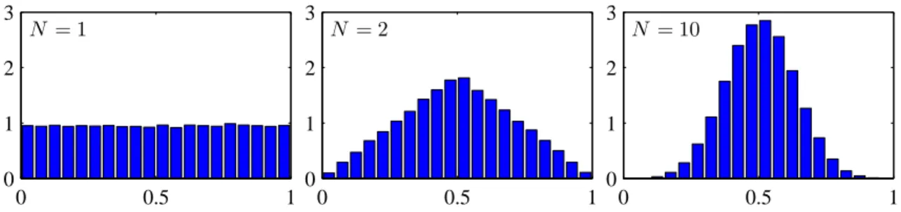
Arguably the single most important PDF is the Normal (a.k.a., Gaussian) probability distribution function (PDF). Among the reasons for its popularity are that it is theoretically elegant, and arises naturally in a number of situations. It is the distribution that maximizes entropy, and it is also tied to the Central Limit Theorem: the distribution of a random variable which is the sum of a number of random variables approaches the Gaussian distribution as that number tends to infinity (Figure 6).

(35)

N = 1

0 0.5 1

0 1 2 3

N = 2

0 0.5 1

0 1 2 3

N = 10

0 0.5 1

0 1 2 3

Figure 6: Histogram plots of the mean ofN uniformly distributed numbers for various values of

N. The effect of the Central Limit Theorem is seen: asN increases, the distribution becomes more Gaussian. (Figure from Pattern Recognition and Machine Learning by Chris Bishop.)

The simplest case is a Gaussian PDF over a scalar valuex, in which case the PDF is:

p(x|µ, σ2) = √ 1

2πσ2 exp

− 1

2σ2(x−µ) 2

(102)

(The notation exp(a) is the same as ea_{). The Gaussian has two parameters, the mean} _µ_{, and}

the variance σ2_{. The mean specifies the center of the distribution, and the variance tells us how}

“spread-out” the PDF is.

The PDF forD-dimensional vectorx, the elements of which are jointly distributed with a the Gaussian denity function, is given by

p(x_|µ,Σ) = p 1

(2π)D_|_Σ_|exp −(x−µ)

T_Σ−1₍_x₋_µ₎_/₂ ₍₁₀₃₎

whereµis the mean vector, andΣis theD_×Dcovariance matrix, and_|A_|denotes the determinant of matrixA. An important special case is when the Gaussian is isotropic (rotationally invariant). In this case the covariance matrix can be written asΣ=σ2_I_where_I_{is the identity matrix. This is}

called a spherical or isotropic covariance matrix. In this case, the PDF reduces to:

p(x_|µ, σ2) = p 1

(2π)D_σ2D exp

− 1

2σ2||x−µ|| 2

. (104)

The Gaussian distribution is used frequently enough that it is useful to denote its PDF in a simple way. We will define a functionGto be the Gaussian density function, i.e.,

G(x;µ,Σ)≡ p 1

(2π)D_|_Σ_|exp −(x−µ)

T_Σ−1₍_x₋_µ₎_/₂ ₍₁₀₅₎

When formulating problems and manipulating PDFs this functional notation will be useful. When we want to specify that a random vector has a Gaussian PDF, it is common to use the notation:

(36)

Equations 103 and 106 essentially say the same thing. Equation 106 says thatxis Gaussian, and Equation 103 specifies (evaluates) the density for an inputx.

The covariance matrix Σ of a Gaussian must be symmetric and positive definite — this is equivalent to requiring that_|Σ_| > 0. Otherwise, the formula does not correspond to a valid PDF, since Equation 103 is no longer real-valued if_|Σ_{| ≤}0.

6.3.1 Diagonalization

A useful way to understand a Gaussian is to diagonalize the exponent. The exponent of the Gaus-sian is quadratic, and so its shape is essentially elliptical. Through diagonalization we find the major axes of the ellipse, and the variance of the distribution along those axes. Seeing the Gaus-sian this way often makes it easier to interpret the distribution.

As a reminder, the eigendecomposition of a real-valued symmetric matrix Σ yields a set of orthonormal vectorsviand scalarsλi such that

Σui =λiui (107)

Equivalently, if we combine the eigenvalues and eigenvectors into matricesU = [u1, ...,uN]and

Λ= diag(λ1, ...λN), then we have

ΣU=UΛ (108)

SinceUis orthonormal:

Σ=UΛUT (109)

The inverse ofΣis straightforward, sinceUis orthonormal, and henceU−1 =UT:

Σ−1 = UΛUT−1 =UΛ−1UT (110)

(If any of these steps are not familiar to you, you should refresh your memory of them.) Now, consider the negative log of the Gaussian (i.e., the exponent); i.e., let

f(x) = 1

2(x−µ)

T_Σ−1₍_x

−µ). (111)

Substituting in the diagonalization gives:

f(x) = 1

2(x−µ)

T_UΛ−1_UT₍_x

−µ) (112)

= 1 2z

T_z ₍₁₁₃₎

where

z= diag(λ−12

1 , ..., λ

−1 2

N )UT(x−µ) (114)

This new functionf(z) = zTz/2 = P_iz2

i/2is a quadratic, with new variableszi. Given variables

(37)

x1

x2

λ1₁/2 λ1₂/2

y1

y2

u1

u2

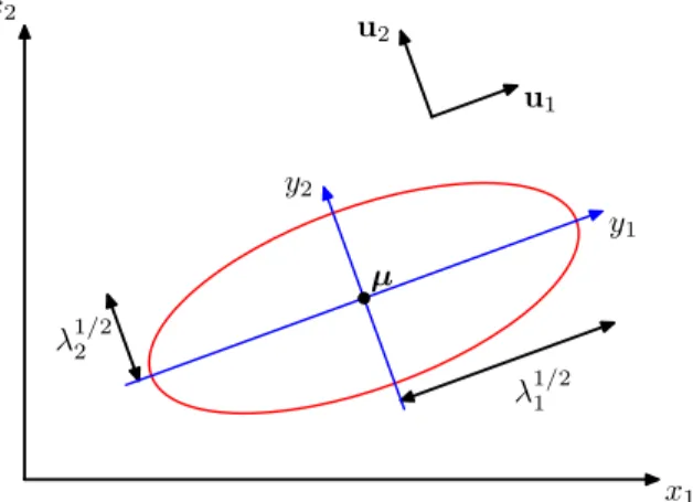
µ

Figure 7: The red curve shows the elliptical surface of constant probability density for a Gaussian in a two-dimensional space on which the density isexp(₋1/2)of its value atx =µ. The major axes of the ellipse are defined by the eigenvectorsuiof the covariance matrix, with corresponding

eigenvaluesλi. (Figure from Pattern Recognition and Machine Learning by Chris Bishop.)(Notey1 and y2in the figure should readz1 andz2.)

nonzero, we can convert back by inverting Eq. 114. Hence, we can write our Gaussian in this new coordinate system as5:

1

p

(2π)N exp

−1 2||z||

2 =Y i 1 √

2πexp

−1 2z 2 i (115)

It is easy to see that for the quadratic form off(z), its level sets (i.e., the surfacesf(z) =cfor constantc) are hyperspheres. Equivalently, it is clear from115thatzis a Gaussian random vector with an isotropic covariance, so the different elements of zare uncorrelated. In other words, the value of this transformation is that we have decomposed the original N-D quadratic with many interactions between the variables into a much simpler Gaussian, composed ofdindependent vari-ables. This convenient geometrical form can be seen in Figure 7. For example, if we consider an individual zi variable in isolation (i.e., consider a slice of the functionf(z)), that slice will look

like a 1D bowl.

We can also understand the local curvature of f with a slightly different diagonalization. Specifically, letv=UT(x₋µ). Then,

f(u) = 1 2v

T_Λ−1_v

= 1 2 X i v2 i λi (116)

If we plot a cross-section of this function, then we have a 1D bowl shape with variance given by

λi. In other words, the eigenvalues tell us variance of the Gaussian in different dimensions.

5_{The normalizing}

(38)

xa xb= 0.7

xb

p(xa, xb)

0 0.5 1

xa p(xa)

p(xa|xb= 0.7)

0 0.5 1

0 5 10

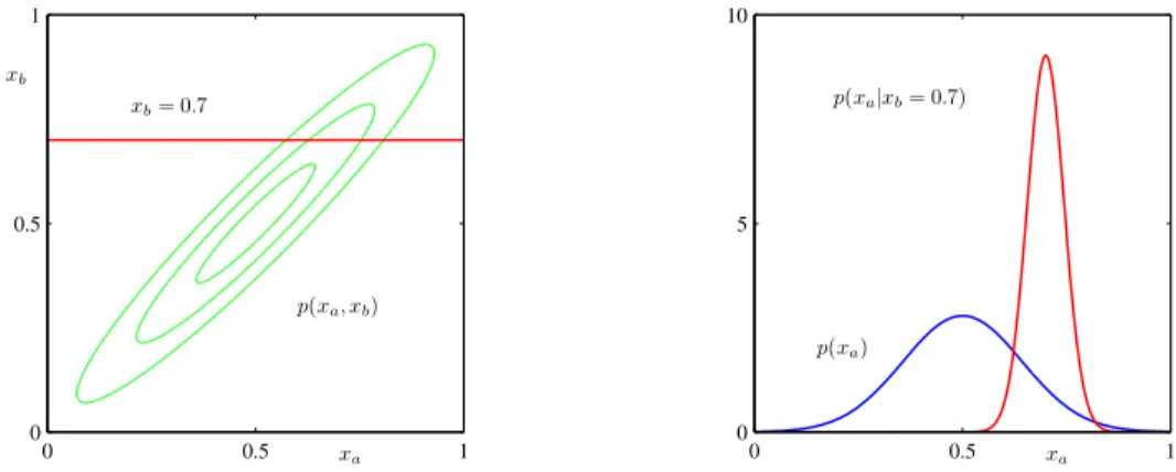
Figure 8: Left: The contours of a Gaussian distribution p(xa, xb)over two variables. Right: The

marginal distributionp(xa)(blue curve) and the conditional distributionp(xa|xb)forxb = 0.7(red

curve). (Figure from Pattern Recognition and Machine Learning by Chris Bishop.)

6.3.2 Conditional Gaussian distribution

In the case of the multivariate Gaussian where the random variables have been partitioned into two setsxa and xb, the conditional distribution of one set conditioned on the other is Gaussian. The

marginal distribution of either set is also Gaussian. When manipulating these expressions, it is easier to express the covariance matrix in inverse form, as a ”precision” matrix,Λ _≡ Σ−1_{. Given}

thatxis a Gaussian random vector, with meanµand covarianceΣ, we can expressx,µ,ΣandΛ all in block matrix form:

x=

x_a

xb

, µ=

µa µb

, Σ =

Σaa Σab

Σba Σbb

, Λ =

Λaa Λab

Λba Λbb

, (117)

Then one can show straightforwardly that the marginal PDFs for the components xa andxb are

also Gaussian, i.e.,

xa ∼ N(µa,Σ_aa), x_b ∼ N(µb,Σ_bb). (118)

With a little more work one can also show that the conditional distributions are Gaussian. For example, the conditional distribution ofxagivenxb satisfies

xa|xb ∼ N(µa|b,Λ−aa1) (119)

whereµ_a_|_b =µa−Λ−_aa1Λ_ab(x_b−µ_b). Note thatΛ−_aa1is not simplyΣ_aa. Figure 8 shows the marginal and conditional distributions applied to a two-dimensional Gaussian.

Finally, another important property of Gaussian functions is that the product of two Gaussian functions is another Gaussian function (although no longer normalized to be a proper density func-tion):

(39)

where

µ= Σ Σ−₁1µ1+ Σ−21µ2

, (121)

Σ = (Σ−₁1+ Σ−₂1)−1. (122)

Note that the linear transformation of a Gaussian random variable is also Gaussian. For exam-ple, if we apply a transformation such that y = Ax where x _{∼ N}(x_|µ,Σ), we have y _∼

(40)

7 Estimation

We now consider the problem of determining unknown parameters of the world based on mea-surements. The general problem is one of inference, which describes the probabilities of these unknown parameters. Given a model, these probabilities can be derived using Bayes’ Rule. The simplest use of these probabilities is to perform estimation, in which we attempt to come up with single “best” estimates of the unknown parameters.

7.1 Learning a binomial distribution

For a simple example, we return to coin-flipping. We flip a coinN times, with the result of thei-th flip denoted by a variableci: “ci =heads” means that thei-th flip came up heads. The probability

that the coin lands heads on any given trial is given by a parameterθ. We have no prior knowledge as to the value ofθ, and so our prior distribution on θis uniform.6 _{In other words, we describe}_θ

as coming from a uniform distribution from 0 to 1, sop(θ) = 1; we believe that all values ofθare equally likely if we have not seen any data. We further assume that the individual coin flips are independent, i.e.,P(c1:N|θ) = Q_ip(ci|θ). (The notation “c1:N” indicates the set of observations

{c1, ...,cN}.) We can summarize this model as follows:

Model: Coin-Flipping

θ ∼ U(0,1)

P(c=heads) = θ

P(c1:N|θ) = Q_ip(ci|θ)

(123)

Suppose we wish to learn about a coin by flipping it 1000 times and observing the results

c1:1000, where the coin landed heads 750times? What is our belief about θ, given this data? We

now need to solve forp(θ|c_1:1000), i.e., our belief aboutθ after seeing the 1000 coin flips. To do

this, we apply the basic rules of probability theory, beginning with the Product Rule:

P(c1:1000, θ) = P(c1:1000|θ)p(θ) = p(θ|c1:1000)P(c1:1000) (124)

Solving for the desired quantity gives:

p(θ_|c1:1000) =

P(c1:1000|θ)p(θ)

P(c_1:1000) (125)

The numerator may be written using

P(c1:1000|θ)p(θ) =

Y

i

P(ci|θ) = θ750(1−θ)1000−750 (126)

Machine Learning and Data Mining Lecture Notes - Free Computer, Programming, Mathematics, Technical Books, Lecture Notes and Tutorials

Lecture Notes

CSC 411/D11

Computer Science Department

University of Toronto

Version: February 6, 2012

Contents

Conventions and Notation

Acknowledgements

1

Introduction to Machine Learning

1.1

Types of Machine Learning

1.2

A simple problem

2

Linear Regression

2.1

The 1D case

2.2

Multidimensional inputs

2.3

Multidimensional outputs

3

Nonlinear Regression

3.1

Basis function regression

3.2

Overfitting and Regularization

3.3

Artificial Neural Networks

3.4

K

-Nearest Neighbors

4

Quadratics

4.1

Optimizing a quadratic

5

Basic Probability Theory

5.1

Classical logic

5.2

Basic definitions and rules

5.3

Discrete random variables

5.4

Binomial and Multinomial distributions

5.5

Mathematical expectation

6

Probability Density Functions (PDFs)

6.1

Mathematical expectation, mean, and variance

6.2

Uniform distributions

6.3

Gaussian distributions

7

Estimation

7.1

Learning a binomial distribution