Song_unc_0153D_13840.pdf

ENROLLMENT AND STOPPING RULES FOR

MANAGING TOXICITY IN PHASE II ONCOLOGY

TRIALS WITH DELAYED OUTCOME

Guochen Song

A dissertation submitted to the faculty of the University of North Carolina at Chapel Hill in partial fulfillment of the requirements for the degree of Doctor of Public Heath in the

Department of Biostatistics.

Chapel Hill 2013

Approved by:

Anastasia Ivanova, PhD Jason Fine, PhD

iii

ABSTRACT

GUOCHEN SONG: Enrollment and Stopping Rules for Managing Toxicity

in Phase II Oncology Trials with Delayed Outcome

(Under the direction of Dr. Anastasia Ivanova)

iv

ACKNOWLEDGMENTS

I would like to thank Dr. Anastasia Ivanova for her continuous encouragement and assistance during this research and thank her for introducing the clinical monitoring field to me and sharing her extensive knowledge within this field with me. I’m grateful to Dr. Olga Marchenko, my manager at Quintiles, for her support and encouragement in the past one year and half. I’m thankful to Dr. Moschos, co-author on one of the papers, from whom I learned a lot about how to communicate with professionals that are not statisticians, and to Mr. Samuel Middleton, who helped to improve the readability of the paper. I would like to thank Dr. Bajat Qaqish, who provided useful comments on the Bayesian approach, Dr. Michael Hudgens for making valuable suggestions on how to improve the document, and Dr. Jason Fine, who kindly found time for my final exam despite his grading obligations. My thanks are extended to Dr. Follmann at NCI with whom I had communication that helped in developing the Bayesian Chapter.

The research was supported in part by NIH grant RO1 CA120082-01A1. I thank Drs. Stergios Moschos, Thomas Shea and Matt Foster for the permission to use the LCCC studies as examples.

v

vi

TABLE OF CONTENTS

LIST OF TABLES ... viii

LIST OF FIGURES ...x

CHAPTER 1 LITERATURE REVIEW ...2

1.1 Introduction ... 2

1.2 Frequentist stopping boundaries ... 2

1.3 Bayesian stopping boundaries... 8

1.4 Stopping boundary in trials with delayed outcomes ... 11

1.5 Enrollment rules ... 13

CHAPTER 2 SHOULD PHASE II TRIALS ROUTINELY REQUIRE STOPPING RULES FOR TOXICITY? ...16

2.1 Overview ... 16

2.2 Introduction ... 17

2.3 Bayesian stopping rule ... 21

2.4 The Pocock versus O’Brien Fleming stopping boundaries... 24

2.5 Comparison of the stopping boundaries ... 27

2.6 Stopping rules we do not recommend using ... 28

vii

2.6.2 Stopping rule based on the upper bound of a confidence

interval ... 29

2.7 CONCLUSIONS ... 30

CHAPTER 3 FREQUENTIST ENROLLMENT AND STOPPING RULES FOR MANAGING TOXICITY REQUIRING LONG FOLLOW-UP IN PHASE II ONCOLOGY TRIALS ...32

3.1 Overview ... 32

3.2 Introduction ... 32

3.3 Stopping for toxicity based on partial data ... 34

3.4 Enrollment rule to prevent an excessive number of toxicities ... 39

3.5 Simulation results and discussion of design parameters ... 43

3.6 Example ... 47

3.7 Conclusions ... 48

CHAPTER 4 BAYESIAN ENROLLMENT AND STOPPING RULES FOR MANAGING TOXICITY REQUIRING LONG FOLLOW-UP IN PHASE II ONCOLOGY TRIALS ...49

4.1 Overview ... 49

4.2 Introduction ... 49

4.3 Bayesian stopping boundary for a trial with immediate response ... 52

4.4 Stopping boundary for trials with delayed outcome ... 56

4.5 Enrollment rule for trials with long follow-up ... 60

4.6 Simulation results and example ... 62

4.7 Discussion ... 67

viii

LIST OF TABLES

Table

2.1. Stopping boundaries for a trial with 20 patients in a trial with acceptable DLT rate of

θ

₀ = 0.2. The trial is stopped after k patients if the number of observed DLTs in equal to

a higher than the corresponding value of the boundary. ... 24 2.2. Operating characteristics of the Pocock boundary with 20

patients, tolerable DLT rate of

θ

₀ = 0.2 and the type I

error rate of 0.05 ... 26 3.1. The Pocock stopping boundary { }b_k for K = 30,

θ

₀ =0.2

and

φ

=0.05 yielding

α

= 0.0164 nd the Pocock

enrollment boundary { }b_k′ with

α

’ _{= 0.0030 ... 37}

3.2. Comparing the new stopping rule that uses all available data when time to toxicity is uniformly distributed in (0, t*) (Uniform) and exponentially distributed with mean

-t*/ln(1-

θ

₀) (Expon) with the rule that uses fully followed patients only (Full data) for a trial that K = 30,

θ

₀ = 0.2, and t* = 12 weeks with one patient being enrolled every week. For comparison we show results for a trial with instantaneous response (t* = 0). We display the probability of stopping the trial early, the expected number of patients,

and the expected number of toxicities ... 38 4.1. Stopping boundaries that yield probability of stopping of 0.05

when toxicity rate is θ = 0.2 and N = 20. Bayesian stopping

boundaries are defined by the priorBeta m m(

θ

, (1−

θ

)) ... 54 4.2. Values

c

to generate the stopping boundary with priors

Beta(3

θ

, 3(1-

θ

)) and Beta(12

θ

, 12(1-

θ

)) _,

θ

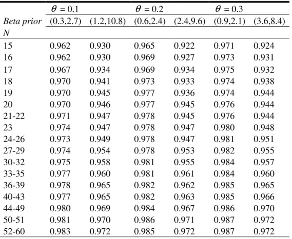
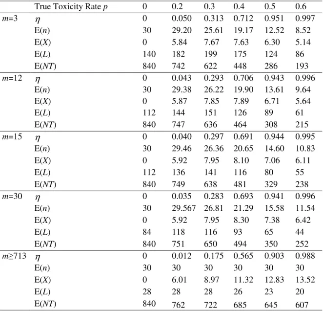
= 0.1, 0.2, 0.3

for various values of the total sample size N ... 62 4.3. Probability of stopping (

η

′), expected number of patients

ix

K = 4, t* = 28 days and the probability of stopping

x

LIST OF FIGURES

Figure

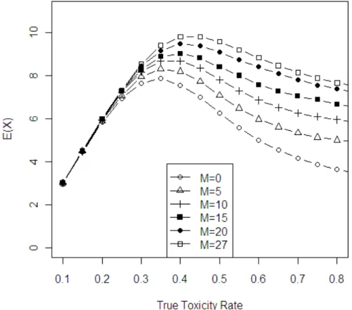
3.1. Expected number of toxicities plotted versus true toxicity rate for different values of M in a trial with K = 30,

θ

₀ =0.2

and

ϕ

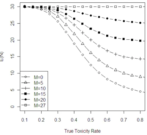
= 0.05. ... 44 3.2. Expected number of patients enrolled in the trial versus

true toxicity rate for different values of M in a trial with K = 30,

θ

₀ =0.2 and

ϕ

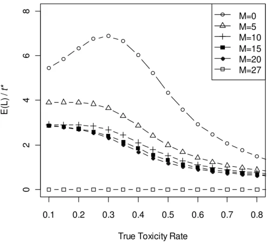
= 0.05. ... 45 3.3. Expected length of study versus true toxicity rates for values

of M in a trial with K = 30,

θ

₀ =0.2 and

ϕ

= 0.05. ... 46 4.1. Expected number of toxicities E(X) vs. true toxicity rate in a

trial with N = 30 patients, for different values of m defining a and b in enrollment rule (4). When m = 3, the trial is the same as a fully sequential trial and when m = 713, enrollment

rule allows to enroll all the patients at once. ... 65 4.2. Expected length in terms of follow-up time for toxicity

T E(L)/ t* vs. true toxicity rate in a trial with N = 30 patients for different values of m in enrollment rule (4). When m = 3, the trial is the same as a fully sequential trial and when m = 713,

CHAPTER 1

LITERATURE REVIEW

1.1Introduction

2

2004). The study applied a Simon-two stage design (Simon, 1989) where the study would only continue if 1 out of the first 14 patients responded to treatment, and the study would conclude that the treatment does not worth further investigation if fewer than 4 responders at the end of the trial. The trial had 4 responses after 21 patients were registered and 15 patients were evaluable, but accrual was terminated because there were too many toxicities observed in these 15 patients: 11 grade IV neutropenia were reported (73%) and additional 2 patients experienced grade III neutropenia. If a stopping rule was in place, these trials would have stopped early and fewer patients would have been exposed to the toxic treatment.

A stopping rule alone does not prevent a trial from possibly observing too many toxicities. An enrollment rule should be used together with a stopping rule to prevent an excessive number of toxicities in phase II trials. In this research, we propose such strategies to improve the current practice of phase II oncology trials.

The document is organized as follows: in Chapter 1, we present literature review. In Chapter 2, we review continuous monitoring rules currently used in phase II designs and give recommendations on which ones are preferred. In Chapter 3, we develop the enrollment strategies and stopping rules using a frequentist method, and in Chapter 4, we propose a Bayesian enrollment strategy and stopping rule.

1.2Frequentist stopping boundaries

Let

θ

be the probability of experiencing toxicity during the follow-up period of the study for a patient at the dose chosen for the study and let

θ

₀ be the probability of

3

to specify the shape of the stopping boundary and the probability of stopping the trial for a given value of

θ

. Ivanova, Qaqish and Schell (2005) examined two types of boundaries widely used in sequential analysis, the Pocock (1977) boundary and the O’Brian-Fleming (1979) boundary, and concluded that the Pocock boundary is the most suitable boundary to monitor toxicity in a phase II oncology trial as it allows stopping early with high probability and, therefore, reduces the expected number of toxicities in the trial.

Let K be the sample size planned for a phase II study. The Pocock boundary can be defined through a point-wise probability

α

₀, such that the trial is stopped if, at each

interim analysis, the null hypothesis

θ θ

= ₀ is rejected at level

α

₀ in favor of the

one-sided alternative

θ θ

> ₀. The value of

α

₀ is chosen so that the overall probability of

stopping the trial,

φ

, is equal to a specified value, usually

φ

=0.05 if the probability of

toxicity is equal to the acceptable rate

θ

₀. We refer to the boundary that allows stopping

the study at any point as a continuous boundary, because monitoring for toxicity is done throughout the trial on a continuous basis. Such a boundary can be described through the sequence of integers (b1, b2, …, bK), which can be computed using step-wise significance

level

α

₀ . The constants bk, k = 1,…,K, are equal to the smallest integer such that

[

k

]

0

P Y b

≥

≤

α

, where Y denotes a binomial random variable with parameters k and

θ

₀. If

the number of toxicities in the first k patients is equal to or higher than bk, the trial is

stopped. Another way of implementing this boundary is to compute a one-sided p-value to test the null hypothesis

θ θ

= ₀ versus a one-sided alternative

θ θ

> ₀ after each patient

is enrolled and their outcome is observed. The trial is stopped if the p-value is less than

0

4

0

α

and the corresponding boundary can be calculated at

http://cancer.unc.edu/biostatistics/program/ivanova/.

The Pocock boundary is a boundary that is constant in the standardized test statistic Z. The O’Brien-Fleming boundary is constant in the B-value defined as

/

Z k K , where k is the number of patients enrolled at the time of the analysis. If the test statistic is a random variable with normal distribution, the step-wise significance level for O’Brien-Fleming boundary at each stage can be calculated as

α

_k =

/ )

K k , where C K_B( , )

φ

is tabulated value that can be found in Jennison and Turnbull

(2000). As C K_B( , )

φ

is a positive number, clearly

α

_k increases in k. For discrete cases,

the O’Brien-Fleming boundary can be computed through trial and error, using C K_B( , )

φ

obtained from the normal approximation as the initial value.

The performance of the boundary is characterized by the probability of stopping the trial for a given probability of toxicity, the expected number of toxicities and the expected number of patients enrolled. For a binomial outcome, the exact calculation can be done as in Schultz et al. (1973), where the probability of stopping was calculated using a recursive formula by observing that to stop at stage k, the kth patient has to experience toxicity and there has to be exactly bk-1 toxicities before stage k. Given the probability of stopping at each stage,

φ

_k for k=1,2,…K, the expected enrollment can be calculated as

( )

_kK_{1 k} (1 ),

E N

φ

k K

φ

= × + −

=

∑

and the expected number of toxicities is calculated as

E(Y)=E(N)

×

θ

.

In general, for each given K,

φ

_and

θ

₀ , a trial using the O’Brien-Fleming

5

the Pocock boundary. The Pocock boundary results in fewer expected toxicities on average compared to the O’Brien-Fleming boundary and, therefore, is preferred for monitoring toxicity or adverse events.

The practice of establishing stopping boundaries to stop experiments can be traced back to the 1940s in Wald’s work of sequential probability ratio test (SPRT) (Wald, 1945). Assume the likelihood function under the null hypothesis is P0(xk) where

xk is data observed at stage k and the likelihood function under the alternative hypothesis

is P1(xk), the log likelihood ratio test is

.

The stopping boundary can be expressed as (

γ γ

₀, ₁): if log(Λ_k)<

γ

₀, the experiment

stops and accepts the null hypothesis as correct, or if log(Λ_k)>

γ

₁, the experiment stops

and accepts the alternative hypothesis as correct. Otherwise, the experiment keeps going until either

γ

₀ or

γ

₁ is crossed. Denote the type I error rate of the SPRT procedure as

,

α

that is, the probability of the procedure accepting P1 when P0 is true and

β

as the

type II error, the probability of the procedure accepting P0 when P1 is true. The procedure yields power of 1−

β

. _{Note that the SPRT contains two one-sided tests at} each stage, and the type I and type II errors of the whole procedure are gained through summarizing the whole sampling space. It is an open ended test with no sample size pre-specified. The values (

γ γ

₀, ₁) can be computed for any given type I error rate and power.

As the SPRT is an open ended test, it cannot be directly applied to clinical trials. Armitage (1957) proposed methods to restrict the sequential procedures to a pre-specified sample size while retaining the type I error and power. Because the SPRT

(

1 0

)

1

log( ) log ( ) log ( )

k

k i i

i

P x P x

=

6

boundaries are for both lower and upper boundaries, that is, to stop if the toxicity rate is too low or too high, it cannot be applied to toxicity monitoring as the trial would not stop if the current data deems the toxicity is acceptably low. Goldman (1987) proposed using the upper bound of SPRT to stop for adverse events in trials where an adverse event is a binary outcome. Let

θ

_A be the probability of toxicity that is not acceptable.

Given a current sample size k, the expression for the upper boundary for stopping is

0

0 0

ln(1 ) ln [ln(1 ) ln(1 )] (ln ln ) [ln(1 ) ln(1 )]

A

A A

k

e β α θ θ

θ θ θ θ

− − − − − −

=

− − − − − .

The parametersα and

β

are nominal parameters for the two one-sided, open ended SPRT. When used with the fixed maximum sample size and only using the upper boundary, α and

β

might have to be adjusted, through trial and error, to yield desired probabilities. For example, one might want the true type I error rate of the procedure to be

φ

= 0.05.

As efficacy endpoint is usually the primary endpoint of phase II oncology trials, in multi-stage designs, the trial usually stops when there is evidence that the treatment is inactive. Bryant and Day (1995) proposed to monitor response and safety jointly in two-stage or multiple-two-stage designs. Let π be the probability of response of the experimental treatment.In this strategy, the null hypothesis is that the treatment is not safe or effective, specifically, the probability of toxicity is *

0

θ or higher OR the probability of response is

0

π

or lower. The alternative hypothesis is that the probability of toxicity is * A

θ and the

probability of response is

π

_A, where θ_A* <θ₀* and

π

_A>

π

₀. Note that the null hypothesis

7

tolerated probability of toxicity, θ₀, in toxicity monitoring strategies described above.

The study result variables were represented by X=(X11,X12,X21,X22) as defined below:

Toxicity No Toxicity

Response X11 X12 Xr

No Response X21 X22 Xr

t

X X_t

The corresponding probability is denoted as (p11, p12, p21, p22). As toxicity and response are bivariate binomial variables, an association variable is needed to fully specify the distribution. The odds ratio between response and toxicity

ϕ

= p p_{11 22}/ (p p_{21 12})was used.

The stopping boundary is a pair of numbers (cr, ct) at stage k, and the trial stops if either

more than ct toxicities or less than cr responses observed out of the number of patients at

stage k. As this rule was usually applied for two stage or three stage designs, it is not a continuous monitoring rule and hence the number of patients at stage k is larger than k. The stopping rule was gained through enumerating all possible pairs of (xr, xt) and the

pair (xr, xt) that satisfies the following situations can be set as the boundary: the

probability of recommending an ineffective but safe treatment,

* 0

[ _{r r}, _{t t}| , _A, )

P X ≥x X ≤x π ≤π θ θ ϕ= is smaller than

α

_R, the probability of

recommending an effective but toxic drug, i.e., * 0

[ r r, t t| A, )

P X ≥x X ≤x π =π θ θ≥ is

smaller than

α

_T,and the power, *

[ _{r r}, _{t t}| _A, _A)

P X ≥x X ≤x π =π θ θ= is at least1−

β

. The

8

calculated for the given

α α

_R, _T, 1−

β

_{by maximizing over}

ϕ

, and the boundary that

gives the smallest such sample size is chosen as optimal.

Conaway and Petroni (1995) developed a similar method, but instead of controlling

α

_R and

α

_T, they proposed to control both the type I error rate over the whole null hypothesis region and the type I error rate at the point null hypothesis. Tournoux et al. (2007) compared the two methods and recommended to use Bryant and Day because it is more flexible. Jin (2007) proposed a method to control the type I error of toxicity and type I error of response separately.

Ray and Rai (2011, 2013) examined to apply the continuous monitoring Pocock boundary (Ivanova et al., 2005) with the Simon’s two-stage (Simon, 1989) design. As the correlation between toxicity and response was ignored at the design stage, the authors found from simulation studies that the procedure was unexpectedly conservative, i.e., trials were stopped more often than desired, when the correlation between toxicity and response is high.

1.3Bayesian stopping boundaries

Geller et al. (2005) proposed a Bayesian stopping rule for continuous monitoring of toxicity. Let Ydenote the number of toxicity events with Y ~ binomial n( , )

θ

, where

θ

is the probability of toxicity and n _{is the number of evaluable patients. Instead of treating}

θ

as a fixed parameter that needs to be estimated, the Bayesian approach assumes that

θ

follows a Beta distribution. Before the trial, the prior distribution is defined as ~Beta a b( , )

9

equivalent to data from

a b

+

patients with mean toxicity a/(a+b), that is, if a prior patients had toxicity and

b

prior patients completed the trial without toxicity. Note that neither a nor

b

has to be an integer. The posterior distribution of

θ

follows a Beta distribution _{where is the number of patients in the current trial}

with toxicity and is the number of patients who have completed the current trial without toxicity. The posterior mean of the toxicity rate is

From the posterior distribution, the probability of the

θ

exceeding a critical value θ₀ can

be computed as follows:

The stopping rule is constructed such that if this posterior probability is larger than a cut-off, the trial stops. Note that the quantity on the right hand side of the formula increases as x increases. For any given n, one can find the smallest x that satisfies the above equation for a pre-specified cutoff value (e.g, 95%). The sequence of such values of x forms the monitoring boundary. In a peripheral blood stem cell trial where 28 patients were planned (Geller et al., 2005), the rate of transplant related mortality (TRM) was monitored using this rule. They set

θ

₀ =0.2 _{and the cutoff for posterior probability as 0.9,}

i.e., the trial stops if the posterior probability that the TRM rate is above 0.2 is greater than 90%. The prior was chosen to worth 6 patients with the mean TRM rate as 0.2, i.e., the Beta (1.2, 4.8) prior was used.

( , ),

Beta a+x b+K−x x

K−x

( )

(

)

(

)

E a x .

a b K

θ = +

+ +

(

)

0

1

0| { | , } .

P Data Beta a x b K x d

θ

10

The operational characteristics of the stopping rule can also be calculated based on Schultz et al. (1973). For example, the probability of stopping is 15.5% and the expected toxicity is 5.17 when the true toxicity rate is 0.2 using this boundary. This Bayesian approach generates a boundary very similar to the Pocock boundary when a non-informative or weakly informative prior is used and the type I error rate is controlled at the similar level.

Etzioni and Pepe (1994) developed a stopping rule to monitor two specific adverse outcomes at the same time and defined excessive toxicity as either type of adverse outcome exceeds a predefined level. In their example of a marrow transplant study, the dose limiting toxicity was defined as either non-engraftment or relapse. Tolerable probability of non-engraftment,

θ

₁, was set at a1 = 30% and the probability of

relapse,

θ

₂, at a2 = 50%. The adverse outcomes were assumed to be independent and

each follows a binomial distribution, given the probability of toxicity

θ

₁ and

θ

₂. A

piecewise uniform prior were placed on probability of toxicity

θ

₁ and

θ

₂: the prior

density is 1/(2a1a2) if

θ

1≤a1 and

θ

2 ≤a2 , and 1/(1/2(1-a1a2)) otherwise. The joint

posterior distribution is a product of Beta densities and hence traceable. The posterior probability of excessive toxicity can be used to monitor excessive toxicities for any given number of patients, the boundary thus is a continuous monitoring boundary.

Instead of controlling the probability of stopping when the probability of toxicity is tolerable, Yu et al. (2012) proposed to stop the trial when there is evidence that the probability of toxicity is at a certain pre-specified high level

θ

₁ . They argued that

11

boundary, are not suitable. They proposed a group sequential strategy to control the incidence rate of toxicity in the study at a certain level. The frequentist boundary at stage k is the largest s_k that satisfies P X

(

_k > Nθ₁−s_k |θ

)

>ξ,where N is the total number of patients in the trial,

ξ

_{is a predetermined constant (suggested to be 0.5 by the authors),}

k i

s ≤n is a non-negative integer and ni is the number of patients in stage i, Xk~Bin(

1 k

i i

N−

∑

₌ n ,

θ

) is a binomial random variable. In the case previous information is

available, they proposed a Bayesian variation of this method by putting a Beta prior on

θ

.

Because existing information is used, the Bayesian version on average enrolls much less patients if the true toxicity rate is high, hence is more effective. The advantage of the proposed boundary are not clear. For example, we compared a boundary from Yu et al. (2012) with

θ

₁ = 0.3, with the Pocock boundary constructed as described in Ivanova et

al. (2005). The Pocock boundary yields better operational characteristics than the boundary in Yu et al. (2012).

For normally distributed outcomes, Freedman and Spiegelhalter (1989) considered trials with up to 5 stages and showed that a Bayesian stopping boundary can have a shape similar to the O’Brien-Fleming or Pocock boundaries depending on the prior, with Pocock boundaries arising from non-informative or slightly informative priors.

1.4Stopping boundary in trials with delayed outcomes

12

otherwise, where t* is the follow-up time for toxicity. When t* is long, it is desirable to make intermediate decisions in the trial based on all the data, including data from patients still under follow-up. Such methods have been developed for phase I oncology trials with long follow-up (Cheung and Chappell, 2000; Ivanova et al., 2007; Bekele et al., 2008).

For example, Cheung and Chappell (2000) developed the time-to-event continual reassessment method (TITE-CRM) in phase I dose finding studies to prevent patients from being assigned to a dose with an unexpected high toxicity. Let θ be the probability of experiencing toxicity by the end of time t*, and u be the time of follow-up for a patient under observation, u < t*. The contribution of information to likelihood function from this patient can be expressed as a truncated probability, w(u,T)θ, where w(u,T) is a weight function. An obvious choice of such weight function is w = u / t*. Other parameters

besides u and t* can be added to the weight function, for example, the level of dose and dose response curve in a dose finding study. An adaptive weight function may utilize the current number and time of toxicities observed in the study. A similar approach is to use the Kaplan-Meier estimator to define the weight function, which is discussed by Yin (2012).

13

Following Antonick (1974) and Blum and Sursala (1977), Follmann and Albert (1999) used all information available in interim analysis using a Dirichlet-multinomial model. They divided the interval (0, t*) into M intervals and tabulated information about adverse events in each of the intervals, with patients completed the trial falls to the interval M+1. To make the interim decision, they enumerate all possible outcomes for each interval and compute their probabilities. With a Dir( )α _{prior, the posterior}

distribution given the observed enrollment profile will be a mixture of Dirichlet distributions for all possible trial results and the probability of the realization for each possible result can be calculated as weight for this distribution. From the mixture of Dirichlet distributions, the posterior distribution of

θ

can be expressed as a mixture of Beta distributions by summarizing the first M elements of the mixture of the Dirichlet distribution. The posterior probability that

θ

exceeds

θ

₀ can be calculated from this

posterior distribution. When the number of patients in follow-up gets large, this calculation requires large computing resources and Follmann et al. (1999) proposed a data augmentation method to resolve this problem based on Tanner (1992).

Under the Dirichlet-multinomial framework, Rosner (2005) applied Gibbs sampling for monitoring clinical trials comparing two survival curves.

1.5Enrollment rules

14

beginning of the trial and guides further accrual based on the information about toxicity in the trial.

Enrollment strategies are often used in phase I dose finding studies to avoid exposing too many patients to potentially toxic compound. For example, in the traditional or the 3 + 3 design, at most 3 patients are enrolled at a time.

In the context of sequential planning of experiments, Schmegner and Baron (2004) defined a risk function that consists of three components: a loss function, a cost from each individual and a fixed cost for each batch. They defined an optimal sequential plan as a plan that minimizes the expected risk. For a trial that enrolls patients in K batches, if the trial enrolls n_k patients at a time, and the cost for enrolling each patient is

i

c but there is a fixed cost c_b for each batch, the risk function is:

1

( ( ,{ })_k K ( _{i k b}),

k

R=E Lθ b +

∑

₌ c n +c

where L( ,{ })

θ

b_k is the loss function determined by the true toxicity rate and the stopping

15

CHAPTER 2

SHOULD PHASE II TRIALS ROUTINELY REQUIRE

STOPPING RULES FOR TOXICITY?

2.1 Overview

17

frequentist Pocock stopping rule and the Bayesian rule, both of which allow stopping the trial early if toxicity rate is high.

2.2 Introduction

18

To date, ‘unacceptable’ toxicity occasionally seen in phase II trials is commonly managed by frequent (>50%) dose reduction or refusal for further treatment. This approach raises the question whether sufficient statistical power remains to assess if a given dose of the investigational agent for which the trial was specifically designed is actually effective or whether any lack of efficacy is secondary to frequent dose reductions due to toxicity (Maki et al., 2009, Alberts et al., 2012, D'Adamo et al., 2005, Wyman et al., 2006). Frequentist and Bayesian methods have been developed to evaluate both toxicity and efficacy as bivariate (efficacy, safety) variable. Most of the methods are two-stage and range from equal weighing of response and toxicity to designs with variable trade-offs between these two outcomes (Jin 2007, Thall and Cheng, 1999, Conaway and Petroni, 1995, Bryant and Day, 1995, Tournoux et al., 2007). Detecting excessive toxicity early is paramount; evaluating toxicity formally only once during the trial is not sufficient.

19

an important secondary endpoint and was monitored closely in real-time, no particular stopping rules for toxicity were incorporated into the study design. Six treatment-related deaths were observed in the initial cohort of 22 patients and therefore the trial was stopped after stage 1. Even in the face of a known high-risk patient population and treatment regimen, it became clear that the trial exhibited an excessive adverse event rate, even though there also appeared to be an emerging strong efficacy signal and pathologic complete response were seen among multiple patients in the initial cohort, including among patients who later developed grade 5 events. In this trial, a formal stopping rule for adverse event might have assisted the study team in weighing the risk/benefit of the therapy.

20

patients, and if 6 events or more are observed in more than 31 patients. Stopping rules can also be incorporated into more novel phase II designs, such as the phase IB portion of the combined phase I-II trials to monitor extended cohort of patients assigned to the estimated MTD, in which case the stopping rule does not have to be as conservative as the ones applied for a phase II study.

21

2.3 Bayesian stopping rule

Consider an example of a phase II trial with a total of K = 20 patients. This can be a single-stage trial or a two-stage trial where, for example, Simon’s two-stage design (Simon, 1989) is used to test the efficacy endpoint. To set up a stopping rule for excessive dose-limiting toxicity (DLT), one needs to specify an acceptable DLT rate, θ₀. Usually, the acceptable DLT rate θ₀ is the rate of toxicities seen at the MTD in the corresponding phase I trial assuming that each patient can develop only a single DLT and that each patient has completed the study, i.e. complete follow-up exists. For example, the rate at the dose chosen by the 3 + 3 design(Storer, 1989) is 0.20 or 0.25 (Reiner, Paoletti and O’Quigley, 1999).

22

observed and 25 patients have completed the trial without DLT, the posterior distribution of the DLT rate is Beta(4 + 5, 16 + 25) with corresponding mean DLT rate of 0.18. The probability that the DLT rate is larger than 0.2 is now 33%. On the other hand, if 10 DLTs are observed among these 30 patients, the posterior distribution of the DLT rate is Beta(4 + 10, 16 + 20). Therefore the probability that the DLT rate is larger than 0.2 is 90% and the DLT rate is estimated as 0.28.

Geller et al. (2005) proposed a Bayesian stopping rule for continuous monitoring of toxicity. The trial is stopped if the posterior probability of the DLT rate exceeding

θ

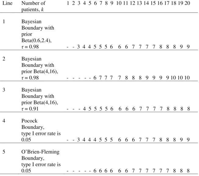
₀ is equal to or higher than a pre-specified value τ. The value of τ is often chosen based on tradition, e.g., 0.95 or 0.98 is commonly seen.

Lines 1 and 2 of Table 2.1 provide two Bayesian stopping boundaries for a trial of 20 patients and τ = 0.98 for

θ

₀ = 0.2. A stopping boundary is described by a set of

integers b1,…, bK such that the trial is stopped if there are bk or more DLTs observed out

of first k patients. The prior distribution, the value of tolerable DLT rate θ0 and the value of τ uniquely define the set of integers b1,…, bK that can be computed before the trial. To

use the Bayesian boundary there is no need to compute the probability that the DLT rate is larger than

θ

₀ = 0.2 given current data, instead one can just check if the number of

observed DLTs in the first k patients is equal to or exceeds bk.

23

probability of stopping the trial when the DLT rate is equal to the acceptable rate of 0.2 is 0.038. The boundary in line 2 of Table 2.1 uses the prior Beta(4, 16), which reflects information from 20 patients with observed DLT rate of 4/20 = 0.20. Since we have strong prior information that the DLT rate is close to 0.20, stronger evidence is needed in the phase II trial that the DLT rate is high to stop the trial compared to the first boundary. This also is reflected in the overall probability of stopping the trial when the DLT rate is equal to the acceptable rate of 0.2, and this probability is very small and is equal to 0.004.

24

Table 2.1. Stopping boundaries for a trial with 20 patients in a trial with acceptable DLT rate of

θ

₀ = 0.2. The trial is stopped after k patients if the number of observed DLTs in equal to a higher than the corresponding value of the boundary.

Line Number of patients, k

1 2 3 4 5 6 7 8 9 10 11 12 13 14 15 16 17 18 19 20

1 Bayesian Boundary with prior

Beta(0.6,2.4),

τ = 0.98 - - 3 4 4 5 5 5 6 6 6 7 7 7 7 8 8 8 9 9 2 Bayesian

Boundary with

prior Beta(4,16),

τ = 0.98 - - - - - 6 7 7 7 7 8 8 8 9 9 9 9 10 10 10 3 Bayesian

Boundary with

prior Beta(4,16),

τ = 0.91 - - - 4 5 5 5 5 6 6 6 6 7 7 7 7 8 8 8 8 4 Pocock

Boundary, type I error rate is

0.05 - - 3 4 4 4 5 5 5 6 6 6 7 7 7 8 8 8 9 9 5 O’Brien-Fleming

Boundary, type I error rate is

0.05 - - - - - 6 6 6 6 6 6 7 7 7 7 7 7 8 8 8

2.4 The Pocock versus O’Brien Fleming stopping boundaries

25

boundary for a given sample size and type I error rate. That is, when used for sequential monitoring of efficacy, the O’Brien-Fleming boundary yields higher probability of declaring the treatment is efficacious when the treatment is indeed effective compared to the Pocock boundary, which is the reason it is used more often. Similarly, when occasionally used to monitor toxicity, the O’Brien-Fleming boundary yields the higher overall probability of stopping the trial compared to the Pocock boundary when the true DLT rate is higher than tolerable. However, the Pocock boundary allows stopping much earlier than the O’Brien-Fleming boundary and therefore it is usually used to stop the trial for adverse events or toxicity. For example, as shown in Table 1, if the Pocock boundary is used, the trial will be stopped if 3 DLTs are observed in the first 3 patients. In comparison, if the O’Brien and Fleming boundary is used, the earliest stopping point requires the first 6 patients all experience DLT.

The Pocock stopping rule can be alternatively described as repeated testing of toxicity rate after each patient completes toxicity follow-up with the null hypothesis that the DLT rate is equal to

θ

₀ = 0.2 and type I error rate

α

'

. This is also equivalent to

using a confidence interval approach. The trial is stopped after k patients if the lower bound of the 1 – 2

α

'

level two-sided confidence interval (Clopper and Pearson, 1934) for DLT rate computed when k patients completed the trial is above

θ

₀ = 0.2. Here

α

'

is

a point-wise α -level. In the Pocock stopping boundary in Table 2.1,

α

'

= 0.0196. For example, if 4 out of 5 DLTs are observed, the 1 – 2

α

'

=

1 – 2 0.0196

×

exact confidence interval for DLT rate is (0.266, 0.996). The lower bound of the interval, 0.266, is higher than

θ

₀ = 0.2, or, in other words the confidence interval does not include 0.2, and

26

trial is stopped. The point-wise α -level,

α

'

, can be computed from a given type I error rate α. Ivanova, Qaqish and Schell (2005) gave a table of values

α

'

for various sample sizes and tolerable DLT rates

θ

₀ . Free software to generate the Pocock stopping

boundary is available at http://cancer.unc.edu/biostatistics/program/ivanova/. For given K,

θ

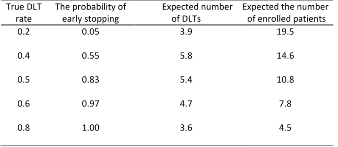
₀ and α, the software computes the stopping boundary and important quantities that

describe the boundary’s performance. For several values of the true DLT rates the program computes the probability of stopping the trial and declaring that the drug is too toxic, the average number of DLTs and the average number of patients in the trial (Table 2.2). For example, when the DLT rate is 0.4 about half of the trials will be stopped (probability of stopping is 0.55). The software also gives an example write-up that can be used in clinical trial protocols.

Table 2.2 Operating characteristics of the Pocock boundary with 20 patients, tolerable DLT rate of

θ

₀ = 0.2 and the type I error rate of 0.05

True DLT rate

The probability of early stopping

Expected number of DLTs

Expected the number of enrolled patients

0.2 0.05 3.9 19.5

0.4 0.55 5.8 14.6

0.5 0.83 5.4 10.8

0.6 0.97 4.7 7.8

0.8 1.00 3.6 4.5

27

2.5 Comparison of the stopping boundaries

As seen from Table 2.1, the Bayesian boundary with Beta(0.6, 2.4) prior and τ = 0.98 is almost indistinguishable from the Pocock boundary. This is true in general: less informative priors, or lower values of a + b, yield Bayesian boundary similar to the Pocock boundary as long as the two boundaries yield similar overall probability of stopping. As the value of a + b increases, that is, the prior becomes more informative, more DLTs are required to occur within the ongoing phase II trial to recommend trial interruption. We need to observe more DLTs to stop the trial because we need to ‘override’ the prior information that toxicity rate is tolerable. In the example in Table 2.1, under the Bayesian rule with informative prior with the probability of stopping of 0.05 (τ = 0.911), we stop later than under the Pocock boundary, but stop earlier than under the O’Brien-Fleming boundary. Another method for stopping due to toxicity we saw in phase II protocols is stopping based on the sequential probability ratio test (SPRT) (Wald, 1945, Armitage, 1957, Goldman, 1987). This method leads to a boundary very similar to the Pocock boundary for given sample size and given actual type I error rate.

If minimal prior information is available, either the Pocock boundary or the Bayesian boundary can be used. Even though they are described by a different statistical language, they are almost identical given the total sample size and the probability of stopping the trial when DLT rate is tolerable. If prior toxicity rate information is available, we recommend using the Bayesian boundary as this prior information can be reflected in the prior distribution for toxicity rate.

28

when θ =

θ

₀, frequentist software at http://cancer.unc.edu/biostatistics/program/ivanova/

can be used to construct the Bayesian boundary. The value τ in the Bayesian boundary can be set to equal to 1 minus step-wise significance level

α

'

corresponding for the common probability of stopping, α , under acceptable DLT rate

θ θ

= ₀ . Software to

construct the Bayesian boundary with the type I error restriction for different type of priors is available from the authors upon request.

2.6 Stopping rules we do not recommend using

In this section we review several stopping rules we have seen in phase II clinical trial protocols that we do not recommend using.

2.6.1 Rule when the trial is stopped as soon as n DLTs are observed

According to this rule the trial is stopped as soon as n DLTs are observed. Despite its simplicity, this rule does not take into account the denominator, that is, the number of patients enrolled in the study at the time of analysis. For example, for a trial with 20 patients and tolerable DLT rate of 0.20, the two rules with the type I error rate closest to 0.05 are ‘stop the trial when 8 DLTs are observed’ with the type I error rate of 0.032 and ‘stop the trial when 7 DLTs are observed’ with the type I error rate of 0.087. Obviously, irrespective of DLT rate, at least 7 or 8 DLTs are to be observed before the trial is stopped. In comparison, the maximum expected number of DLTs under the Pocock boundary is 5.8 when the true DLT rate is 0.4 and less for higher DLT rates.

29

0.05, the trial is stopped if 2 DLTs are observed in the first 2-5 patients, or 3 DLTs are observed in first 6-14 patients, or 4 DLTs are observed in more than 14 patients. This boundary yields less expected DLTs than a constant boundary where the trial is stopped as soon as 3 DLTs are observed. Therefore we recommend using the Pocock or the Bayesian boundary and not the constant boundary.

2.6.2 Stopping rule based on the upper bound of a confidence interval

As mentioned in Section 2.4, stopping according to the Pocock boundary is equivalent to stopping the trial when the lower bound of a confidence interval is above the acceptable DLT rate. In the example in Section 2.4 we compared the lower bound of the confidence interval (0.266, 0.996), 0.266, with

θ

₀. As the purpose of the stopping

30

of the confidence interval is 1 no matter what significance level is used. With 1-2

α

'

= 0.9, for example, if the true DLT rate is 0.2, the trial has the probability of stopping of 0.2 after the first patient and the overall probability of stopping of 0.82 for a trial with 20 patients.

2.7 Conclusions

We reviewed several stopping rules for toxicity we have infrequently seen in phase II trial protocols. We propose to keep the probability of stopping the trial when the DLT rate is equal to the acceptable DLT rate at 0.05 or lower. In such cases, one needs to have rather strong evidence that the DLT rate is high to stop the trial early for toxicity. The goal is to stop the trial as early as possible if there is ‘strong’ evidence of high DLT rate. The term ‘strong’ implies that stopping rules for toxicity should by no means be extremely conservative to the point that they overshadow the main purpose of the phase II study, namely the efficacy assessment. Under this concept we anticipate that stopping rules for toxicity would be activated before efficacy rules infrequently. In addition, we argue that continuous stopping rule for toxicity should be used, that is, the rule that allows stopping the trial at any point. Between the two stopping boundaries most commonly used in clinical trials, the O’Brien-Fleming boundary and the Pocock boundary, we recommend the Pocock boundary as it allows stopping for toxicity as early as possible.

31

given dose in phase I and therefore the information derived from phase I trial is not very relevant), the Pocock or the Bayesian boundary with non-informative prior can be used, as they are virtually identical in this case. If there is reliable prior information about toxicity rate to use in the stopping rule, we recommend using the Bayesian boundary as it is the only boundary that can formally account for prior information about toxicity. On the other hand, prior information has to be used with caution as various factors including the change in patient population might affect the DLT rate of the investigational treatment. Boundaries mentioned in Section 2.6, are not recommended.

CHAPTER 3

FREQUENTIST ENROLLMENT AND STOPPING RULES FOR

MANAGING TOXICITY REQUIRING LONG FOLLOW-UP IN

PHASE II ONCOLOGY TRIALS

3.1Overview

Monitoring of toxicity is often done in phase II trials in oncology to avoid an excessive number of toxicities if the wrong dose is chosen for phase II. Existing stopping rules for toxicity use information from patients who have already completed follow-up. We describe a stopping rule that uses all available data to determine whether to stop for toxicity or not when follow-up for toxicity is long. We propose an enrollment rule that prescribes the maximum number of patients that may be enrolled at any given point in the trial.

3.2Introduction

33

34

Bekele et al. (2008) suggested halting enrollment to a phase I trial when there is not enough data to select a safe dose for the next patient. The problem is different in a phase II context as it is a single arm trial and dose reduction in the middle of the trial will make it difficult, if not impossible, to estimate the efficacy and toxicity of the experimental compound at a certain dose level. The main challenge in a phase II trial with long follow-up for toxicity is to maintain the pre-specified probability of stopping the trial under various true toxicity rates, the type I error rate and power, when partial data are used. Methods for phase I trials with long follow-up for toxicity do not apply in phase II context. However, we use the same assumption as in Cheung and Chappell (2000) to utilize partial data. In this paper in Section 3.3 we describe a stopping rule for toxicity based on partial data. Enrollment strategies are discussed in Section 3.4, the simulation study is presented in Section 3.5, example in Section 3.6 and discussion in Section 3.7.

3.3 Stopping for toxicity based on partial data

In a phase II study each patient is followed for toxicity for a fixed period time of t*. Let n be the number of patients enrolled in the study so far. Let Ui be the random

variable denoting the time to toxicity for the ith patient and let

θ

₌ P(Ui ≤ t*) be the

probability of toxicity. Denote Yi,n the indicator that the ith patient has experienced

toxicity by the time just prior to the entry of the (n+1)th patient, i = 1,…,n, then

, 1 n

n _i i n

X Y

=

=

∑

is the random variable denoting the total number of toxicities observed at

that time.

35

binomial(n,

θ

). Ivanova et al. (2005) considered such trials and argued that the Pocock boundary is the most suitable boundary for monitoring toxicity in a phase II oncology trial as it allows stopping early with high probability and therefore reduces the expected number of toxicities. Let K be the sample size planned for a phase II study and let

θ

₀ be the acceptable probability of toxicity. The Pocock boundary can be defined through a point-wise probability α , such that the trial is stopped if, at each interim analysis, the null hypothesis

θ θ

= ₀ is rejected at level α in favor of the one-sided alternative

θ θ

> ₀.

The value of α is chosen so that the overall probability of stopping the trial,

φ

, _{is equal}

to a specified value, usually

φ

=0.05, if the toxicity rate is

θ

₀. We refer to the boundary

that allows stopping the study at any point as a continuous boundary, because monitoring for toxicity is done throughout the trial on a continuous basis. Let the constants bk, k =

1,…,K, be the smallest integer such that

P X

[

_k

≥

b

_k

]

≤

α

, then such a boundary can be

described through (b1, b2, …, bK). If the number of toxicities in the first k patients is equal

to or higher than bk, the trial is stopped. Another way of implementing this boundary is to

compute a one-sided p-value to test the null hypothesis

θ θ

= ₀ versus one-sided

alternative

θ θ

> ₀ after each patient’s outcome is observed. The trial is stopped if the

p-value is less than α . In fact, it is sufficient to apply the boundary only when a patient has toxicity. We now explain how to use data from partially followed patients to implement a sequential boundary. We will compute the p-value to test the null hypothesis

θ θ

= ₀

versus the one-sided alternative

θ θ

> ₀ based on all information available using

36

Now consider the case when not all n patients are fully followed for toxicity at the time just prior to the entry of the (n+1)th patient. Let ti,n be time elapsed from the start of

treatment for the ith patient at the time just prior to the entry of the (n+1)th patient. Following Cheung and Chappell (2000), for ti,n < t*, we have

,

* *

,

*

, *

, ,

( _{i i n}) ( _{i i n}| _i ) ( _i ) ( _{i in}| _i ) ti n _in .

P U t P U t U t P U t P U t U t w

t

θ

θ

θ

≤ = ≤ ≤ ≤ = < ≤ = =

In other words, a weight wi,n = P(Ui < ti,n | Ui ≤ t*) is assigned to the ith patient and the

probability that the ith patient experiences toxicity when treated for a length of ti,n is wi,n

θ

.

This is equivalent to assuming that the time to toxicity given that toxicity occurs in (0, t*) follows a uniform distribution on the interval (0, t*). This and other weighting options were described in Cheung and Chappell (2000) and Yin (2012). The weight w_{i n,} is set to

1 for patients who have already experienced toxicity and patients who have completed follow-up. At the time just prior to the entry of the (n+1)th patient, the number of patients

who completed the trial without toxicity is _,

1 ( 1)

n

n _i i n n

S =

∑

₌ I w = −X and the number of

patients still under follow-up is _,

1 (0 1)

n

n _i i n

R =

∑

₌ I <w < , X_n +S_n+R_n =n. Let x, s and r

denote the observed Xn, Sn and Rn respectively. The one-sided p-value for testing the null

37

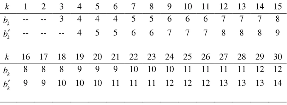
Table 3.1. The Pocock stopping boundary { }b_k for K = 30,

θ

₀=0.2 and

φ

=0.05 yielding

α

= 0.0164, and the Pocock enrollment boundary { }b_k′ with α′ = 0.0030

k 1 2 3 4 5 6 7 8 9 10 11 12 13 14 15

k

b -- -- 3 4 4 4 5 5 6 6 6 7 7 7 8

k

b′ -- -- -- 4 5 5 6 6 7 7 7 8 8 8 9

k 16 17 18 19 20 21 22 23 24 25 26 27 28 29 30

k

b 8 8 8 9 9 9 10 10 10 11 11 11 11 12 12

k

b′ 9 9 10 10 10 11 11 11 12 12 12 13 13 13 14

For example, if n = 3, x = 2,

s

=

1

and

r

=

0

, then all weights are equal to 1 and

the p-value is calculated as

P X

[

₃

≥

x

]

=

P X

[

₃

≥

2

]

= 0.104, where X3 is a binomial

random variable with parameters 3 and

θ

_{0 = 0.2,} X3 ~binomial(3,0.2) . In another

example, the counts right before enrolling the fourth patient are n = 3,

x

=

2

,

s

=

0

and

1

r= with the first two patients fully followed and time

t

_3,3

=

t

*

/ 2

and hence w_3,3 =1/ 2

for the patient still in follow-up, then X₃ =Y_1,3+Y_2,3+Y_3,3, where Y_i,3 ~ Bernoulli( )

θ

₀ for

i =1,2 and Y_3,3 ~ Bernoulli(

θ

₀/ 2). Therefore

[

3

2

]

1,3 2,3

1,

3,3

1

1,3 2,3

1,

3,3

0

0.072.

38

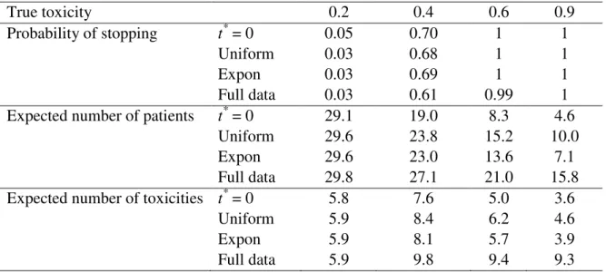
Table 3.2. Comparing the new stopping rule that uses all available data when time to toxicity is uniformly distributed in (0, t*) (Uniform) and exponentially distributed with mean -t*/ln(1-

θ

₀) (Expon) with the rule that uses fully followed patients only (Full data) for a trial that K = 30,

θ

₀ = 0.2, and t* = 12 weeks with one patient being enrolled every week. For comparison we show results for a trial with instantaneous response (t* = 0). We display the probability of stopping the trial early, the expected number of patients, and the expected number of toxicities

True toxicity 0.2 0.4 0.6 0.9

Probability of stopping t* = 0 0.05 0.70 1 1

Uniform 0.03 0.68 1 1

Expon 0.03 0.69 1 1

Full data 0.03 0.61 0.99 1

Expected number of patients t* = 0 29.1 19.0 8.3 4.6

Uniform 29.6 23.8 15.2 10.0

Expon 29.6 23.0 13.6 7.1

Full data 29.8 27.1 21.0 15.8

Expected number of toxicities t* = 0 5.8 7.6 5.0 3.6

Uniform 5.9 8.4 6.2 4.6

Expon 5.9 8.1 5.7 3.9

Full data 5.9 9.8 9.4 9.3

We illustrate the ability of this rule to stop the trial via simulations. Consider an example of a phase II trial with K = 30. To yield the overall probability of stopping of 0.05 when

θ

₀=0.2, we need to use

α

=

0.0164

at each step. The continuous Pocock

39

is high. We repeated the simulations for various patterns of patient enrollment and the results were very similar to those in Table 3.2.

3.4Enrollment rule to prevent an excessive number of toxicities

If many patients are enrolled at once, the stopping rule described in the previous section will not prevent treating too many patients on a regimen that may not be safe. Often, many patients are enrolled at the very beginning of the trial which might lead to excessive toxicities. An enrollment rule informs investigators about how many patients may be enrolled at the beginning of the trial and guides further accrual based on the information about toxicity in the trial.

Consider the boundary in Table 3.1. Initially we may enroll 3 patients as it is not possible to stop the trial before 3 patients complete follow-up. If none of these patients experience toxicity in (0, t*), one may enroll as many as 5 more patients, since there is a possibility to cross the boundary by observing 5 toxicities out of 8 patients, and it is not possible to cross the boundary if less than 5 additional patients are enrolled. More formally, the trial can enroll m new patients such that r + x + m ≤ bn+m,r + x + m – 1 <

40

rather long trial if t* is long. We considered three ways to relax this rule resulting in three different enrollment strategies.

The first enrollment strategy is described as follows. Let M be the design parameter fixed in advance. One can think of M as the number of extra toxicities we are willing to allow to make the trial shorter. The maximum number of new patients to enroll, m, is determined by r + x + m ≤ b_{n m+} +M ,r + x + m - 1<b_{n m+ −1}+M and n + m ≤

K. That is, at any time the maximum number of patients experiencing toxicity cannot

exceed the number allowed by the Pocock boundary plus M. As before we assume the worst case scenario that all patients will experience toxicity and allow M extra toxicities beyond what is allowed by the Pocock boundary. When M = 0, the rule is equivalent to the conservative enrollment plan. The maximum number of patients to enroll in the trial initially is b* + M, where b* is the minimum number k such that k ≥ _{bk. In the example in} Table 3.1, we can enroll at most 3 + M patients initially. If M is as large as M ≥ _{K – b}*_{, all} patients can be enrolled in the beginning of the study.

The second enrollment strategy we consider is to use a separate Pocock boundary for enrollment, the boundary that yields the overall probability of stopping the trial of

φ

′,

φ

′ ≤

φ

, or step-wise probability

α

′

in place of α ,

α

′ ≤

α

, when θ =θ₀.Let { }b_k′ be the

set of constants corresponding to the second Pocock boundary. The number of patients we are allowed to enroll, m, is such that r + x + m ≤ b_{n m}′₊ ,r + x + m – 1 < b_{n m}′_{+ −1} and n +

m ≤ K. An example of an enrollment boundary { }b_k′ with

α

′ =

0.003

is shown in Table

41

= 5, b₇′ = b₈′= 6, we get m = 1 and therefore we may enroll one more patient. If

φ

′ =

φ

,

the rule is equivalent to the conservative enrollment plan.

In the third enrollment strategy a patient completed t / t* of the total follow-up contributes 1−t/t* toxicity to the total toxicity count we will use to calculate allowable enrollment. The total toxicity count,

ξ

, just prior to the entry of the (n+1)th patient is x plus the sum of *

,

1−ti n/t , where the sum is over all the patients still in the follow-up.

Similarly to how it was done in Section 3.3, one can compute the p-value to test

θ θ

= ₀

given

ξ

+m toxicities out of n + m patients. The maximum number of patients one may enroll is the maximum m such that m≤K−n and

[

|

~ binomial( ,

0

)

]

P X

≥ +

ξ

m X

θ

n m

+

≤

α

.

In the beginning of the trial, this enrollment rule is the same as the conservative enrollment plan since

ξ

= 0 and n = 0. In the example in Table 3.1, say, if there are 2 toxicities observed, 1 patient completed the trial without toxicity and 3 patients are right in the middle of the follow-up, then

ξ

= 2 + 3×0.5 = 3.5 and n = 2 + 1 + 3 = 6.

Calculating the probability

P X

[

≥

3.5

+

m X

|

~

Binomial

(0.2,6

+

m

)

]

for various m and

42

We examined all three strategies. All three strategies allow flexibility as one can vary parameters M,

α

′

and θ correspondingly. In the trial in Table 3.1, choosing M = 1, for example, has very similar results to the second strategy with

α

′ =

0.0030

, and choosing M = 3 has very similar results to the second strategy with

α

′ =

0.0003.

Choosing M = 2 in the first strategy is similar to the third strategy with θ =1. The third strategy utilizes the partial data in the trial better than other strategies but it is substantially more complex to implement as it requires real time calculations. The first two strategies do not require complex real time calculations and can be easily implemented during the trial according to specifications in a clinical trial protocol. Also the first strategy has a clear interpretation as allowing at most M additional toxicities over the stopping rule. As the performance of the three strategies is similar, we recommend the first enrollment strategy because of its simplicity. We will refer to this strategy as +M enrollment rule in the remainder of the paper.

As mentioned earlier, using just the stopping or just the enrollment rule will not prevent the trial from possibly seeing excessive toxicity. The algorithm below describes how to apply both the stopping rule from Section 3.3 and the +M enrollment rule described in this Section in a clinical trial.

(i) Initial enrollment is b* + M. For example, in Table 3.1, b* = 3.

(ii) When toxicity is observed, calculate the p-value as described in Section 3.3. If p-value is less than α , stop the trial.

(iii) When there is a toxicity or a patient reached the end of follow-up t* without toxicity, if x r+ ≥b_{x s r+ +} +M, no new patients may be enrolled. If

x s r

43

integer

m

that satisfies

m b

=

_{x s r m+ + +}

+

M

−

(

x r

+

)

. If m > + +x r s then enroll

( )

K− x r+ +s patients, otherwise, enroll

m

patients.

3.5Simulation results and discussion of design parameters

In this section we present a simulation study investigating the performance of the +M enrollment rule for various values of M in conjunction with the stopping rule described in Section 3.3. We used the example from Section 3.3 with K = 30 and

θ

₀ =0.2

. Figures 3.1-3.3 show the expected number of toxicities, expected number of patients enrolled and expected length of trial (in units of t*) for some values of M across the range of true toxicity rate. When

M

=

0

the probability of stopping the trial is almost the same as

φ

. As M increases, assuming that patients are always available to enroll in the trial, the probability of stopping the trial decreases slightly. At the same time, the expected number of toxicities is increasing mostly because many more patients are enrolled before the trial is stopped and not because the probability of stopping gets slightly lower than with

0

44

45

46

0.1 0.2 0.3 0.4 0.5 0.6 0.7 0.8

0

2

4

6

8

True Toxicity Rate

E

(L

)

/

t*

M=0 M=5 M=10 M=15 M=20 M=27