Taxation and Inequality: Active versus Passive Channels
∗
Estelle Dauchy
†Nathan Seegert
‡Abstract
We evaluate the ability of the income tax to insure household consumption against income shocks. To do this, changes in insurance are decomposed into active insurance changes (due to changes in the tax code), passive insurance changes (due to changes in the income distribution), and residual behavioral insurance changes. From 1967 to 2010, both active and passive insurance changes had large, partly offsetting effects, such that the overall effect on insurance was minimal. In particular, active insurance changes decreased insurance and passive insurance changes increased insurance suggesting that, tax policy and the nonlinearity of the tax code influence consumption inequality.
Keywords: inequality, personal income taxation, income risk, consumption JEL: D12, D31, D91, H24, E21
∗We thank Luis Rayo, Byron Lutz, and Ramen Molley for the very valuable comments. We are grateful to Alan Feenberg of the National Bureau of Economic Research for his help compiling certain CEX years, Alexey Khazanov for excellent research assistance, as well as seminar participants at the New Economic School in Moscow, Drexel University in Philadelphia for their helpful comments.
†[email protected]. Campaign for Tobacco Free Kids, 1400 I (Eye) Street NW, Suite 1200, Washington, DC 20005.
1
Introduction
The recent rise in income and consumption inequality in the United States has been a national topic of concern.1 Previous studies place income taxation at the center of the
debate on income and consumption inequality because it has the potential to reduce the transmission of income shocks to consumption.2 The public finance literature finds that
decreases in the progressivity of the income tax had a large impact on the distribution of income between 1980 and 2007 (Bargain and Siegloch, 2014; Piketty and Saez, 2007). This suggests that the transmission of income shocks to consumption should have increased—but the empirical evidence finds no change in the transmission of income shocks to consumption (Blundell, Pistaferri, and Preston, 2008). This poses a puzzle that despite important tax policy changes in this period, the transmission of income shocks to consumption did not change. If true, this would suggest that income tax policy may be unable to combat the rise in consumption inequality.
This puzzle leads us to investigate two open questions in this literature, how much does income taxation damp consumption inequality and what are the mechanisms by which tax policy impacts the transmission of income shocks to consumption. To answer these questions, we investigateactive andpassiveinsurance changes. Activechanges are due to changes in tax policy. Passive changes are due to changes in the income distribution and how it interacts with the nonlinear structure of the income tax schedule. Both active and passive changes impact the transmission of income shocks to consumption.
A simple thought experiment helps to clarify active and passive insurance changes. Sup-pose there are two households, with pre-tax incomes of $10,000 and $60,000, respectively. The tax system consists of two brackets such that income below $30,000 is taxed at 15 percent and income above this threshold is taxed at 25 percent. In this baseline scenario, inequality of after-tax income, measured as the coefficient of variation (the standard deviation divided by the mean), is 0.988, compared to the coefficient of variation of pre-tax income of 1.01. Consider an active change in insurance due to an increase in the top marginal income tax rate from 25 to 29 percent. In this scenario, the coefficient of variation of after-tax income 1Several studies in labor, public finance, and macroeconomics have explored whether the rise in inequality
is due to permanent or transitory income shocks, finding important roles for both but at different times. Examples include Blundell, Pistaferri, and Preston (2008); Cutler and Katz (1992); Aguiar and Bils (2011); Altonji and Siow (1987); Attanasio and Pistaferri (2012); P. and Pavoni (2011); Attanasio and Weber (1995). These literatures are discussed in more detail at the end of the introduction.
2Many studies of income inequality similarly suggest an important role for taxation, reporting differences
decreases to 0.979, but the coefficient of variation of pre-tax income remains 1.01. Now consider apassive change in insurance due to a 10 percent increase in the income levels. The coefficient of variation of after-tax income decreases to 0.986. In this scenario, even though the tax system did not change, it contributed to an increase in insurance and a decrease in inequality.
We find that active tax policy changes decreased insurance to permanent and transitory income shocks by 45 and 24 percent, respectively, between 1968 and 2010. In contrast, passive tax policy changes increased insurance to permanent and transitory income shocks by 32 and 16 percent, respectively. Taken together, the combined effect of the income tax on insurance is minimal, consistent with the illustrative evidence by Blundell, Pistaferri, and Preston (2008) and Debacker and Vidangos (2013). However, this total effect obscures substantial effects from active and passive insurance changes on insurance.
Our approach makes several advances to separately identify active and passive tax policy changes. First, we extend the sample period typically studied (1980–1992) to the years 1967–2010. To do this, we combine data from the Panel Study of Income Dynamics (PSID) and the consumer expenditure survey (CEX). We find large changes in the transmission of income shocks to consumption between the periods 1967–1979, 1980–1992, and 1993–2010, that are not observable in the smaller period typically studied.3
Second, we develop measures of changes in insurance due to active and passive tax policy changes. We calculate these measures using simulations of after-tax income from the NBER’s TaxSim software. Active insurance changes are calculated by simulating the changes in insurance a household would have received if its income had not changed (in real terms) while tax policy had changed as observed. Passive insurance changes are calculated by simulating the change in insurance a household would have received if tax policy had not changed while its income had changed as observed (and deflated to dollars in a base year). We find large and opposite changes in active and passive insurance from 1968 to 2010.
Third, we derive a decomposition that quantifies the impact of changes in active and passive insurance on the transmission of income shocks to consumption. We start from a standard micro model of the joint distribution of income and consumption. We then add taxes to the model to derive a structural relationship between changes in active and 3We report our estimates using the periods 1967–1979, 1980–1992, and 1993–2010 because these years
passive insurance and the transmission of income shocks to consumption. This structural relationship allows us to decompose the total change in insurance into the change due to active insurance changes, passive insurance changes, and residual behavioral changes. We define behavioral changes as all other changes in insurance, such as changes in household’s propensity to consume tax refunds and changes in credit availability. To the best of our knowledge, such a decomposition on the transmission of income shocks to consumption has not been done.
Our findings suggest two future policy considerations. First, tax policy changes can sub-stantially influence the transmission of income shocks to consumption. Second, the nonlinear structure of the income tax damps inequality, and acts as an automatic counter to rising before-tax income inequality.
Related Literature
Through research across fields, we know several facts about income and consumption dynamics over the last forty years. First, income inequality has increased over the last forty years. Second, permanent and transitory shocks to income have contributed to the increase in inequality. Third, the increasing trend in consumption inequality is generally smaller than the increasing trend in income inequality. Fourth, the tax system provides insurance against income shocks and can damp consumption inequality relative to income inequality.
In this paper, we investigate the next open questions in this literature, how much does income taxation damp consumption inequality and how have tax policy changes impacted the transmission of income shocks to consumption. To answer these open questions, we build on the insights of the previous literature. The following discussion provides some background on the methods and modeling choices in the previous literature.
The macro-labor literature finds that the income process that most closely fits individual income data allows for both permanent and transitory shocks (MaCurdy, 1982; Abowd and Card, 1989; Autor and Kearney, 2008; Meghir and Pistaferri, 2004).4 Some of these models
estimate the evolution of income shocks in levels and some in growth rates. However, both kinds of models show that the sharp increase in income inequality over the past 40 years was driven by both permanent and transitory shocks, with permanent income shocks generally 4More flexible models allow for some consumers to be liquidity constrained, other economic and policy
driving the long-term trend but transitory income shocks showing a large and increasing contribution in the late 1980s and early 1990s (Blundell, Pistaferri, and Preston, 2008; Primiceri and Rens, 2009; Moffitt and Gottschalk, 2011, 2012; Heathcote and Violante, 2010; Debacker and Vidangos, 2013).
Most of these studies use a model-based approach, making assumptions about the income process and the nature of liquidity constraints (MaCurdy, 1982; Abowd and Card, 1989; Autor and Kearney, 2008; Meghir and Pistaferri, 2004). A notable exception is Kopczuk and Song (2010) who use a non-parametric method. Using US Social Security income data, Kopczuk and Song (2010) decompose income shocks into a permanent component, obtained from a five-year moving average of residual income, and a transitory component, obtained from the difference of the true residual income and permanent income. They find that permanent income shocks are an important part of the increase in inequality since at least the 1970s. Debacker and Vidangos (2013) compare the Kopczuk and Song (2010) method and the model-based method, widely adopted by the literature and used in this paper, finding both methods attribute a large portion of the increase in income inequality to permanent income shocks but that the model-based approach attributes more weight to transitory shocks.
Most studies that evaluate the evolution of income shocks over time focus on either male earnings (MaCurdy, 1982; Gottschalk and Moffitt, 2009; Moffitt and Gottschalk, 2002, 2011, 2012; Meghir and Pistaferri, 2004), household incomes (Krueger and Perri, 2005, 2006; Blun-dell, Pistaferri, and Preston, 2008), or both (Heathcote and Violante, 2010; Debacker and Vidangos, 2013).5 This literature generally finds subtle differences in the impact of
perma-nent and transitory shocks on male and household incomes and find transitory income shocks contributed heavily in the late 1980s and early 1990s (Blundell, Pistaferri, and Preston, 2008; Primiceri and Rens, 2009; Moffitt and Gottschalk, 2011, 2012; Heathcote and Violante, 2010; Debacker and Vidangos, 2013).6
The extent to which the increases in permanent and transitory income shocks have led to consumption inequality depends on how much of these shocks are insurable. The fact that the increase in consumption inequality is smoother overall than that of income suggests that consumers can predict and insure against at least part of income shocks (Cutler and Katz, 5In addition to male earnings, household income includes spousal labor earnings, transfer income (e.g.,
alimony, pensions, annuities, unemployment compensation, tax refunds, social security benefits), investment income (e.g., dividends, capital gains), and business income (i.e., income from sole proprietorships, partner-ships, S corporations). Household income is hence likely to more broadly reflect household consumption and welfare.
6Debacker and Vidangos (2013) find that about 20 percent of the total increase in income variance from
1992; Aguiar and Bils, 2011; Altonji and Siow, 1987; Attanasio and Pistaferri, 2012; P. and Pavoni, 2011; Attanasio and Weber, 1995). Moffitt and Gottschalk (2012) and Heathcote and Violante (2010) find the overall increasing trend in consumption inequality is generally smaller than that of income because a non-negligible component of these income shocks is transitory and insurable.7
To better understand the transmission of income shocks to consumption, Blundell, Pista-ferri, and Preston (2008) estimate the size of the transmission of permanent and transitory income shocks to consumption. To do this, they construct a panel database of individual con-sumption and income from the PSID and the CEX from the early 1980s to the early 1990s. They show that the degree of consumption insurance significantly depends on whether in-come shocks are permanent or transitory. They find little evidence the level of insurance varied over their sample years, 1980–1992. Instead, they suggest that the increase in con-sumption smoothing in the late 1980s and early 1990s was due to increases in transitory shocks, which are transmitted to consumption less.
Blundell, Pistaferri, and Preston (2008) provide additional evidence suggesting that the tax system is an important determinant of the transmission of permanent income shocks to consumption.8 Covering a longer period up to the financial crisis, Heathcote and Violante (2010) and Debacker and Vidangos (2013) evaluate the variability of before-tax and after-tax income shocks, attributing the difference to the tax system.9 They find suggestive evidence that the tax system contributed to insure against permanent income shocks since the 1980s 7The macroeconomic literature has extensively studied the transmission of income shocks to consumption,
with a particular attention to the validity of the permanent income hypothesis (PIH), as opposed to other models of buffer-stock savings, impatient consumers, or models with liquidity constraints (Zeldes, 1989; Carroll and Kimball, 2001). While the PIH implies that forward-looking consumers fully adjust consumption in response to permanent shocks and unconstrained consumers, fully insure transitory shocks, impatient or constrained consumers are subject to both permanent and transitory income shocks. Carroll (2009) applies various models of consumers behavior under constraints to PSID data and finds that, although the marginal propensity to consume out of permanent income shocks is always less than one, the PIH is approximately right: across a wide range of assumptions on the degree of impatience, marginal propensity to consume out of permanent income shocks between 0.75 and 0.92.
8Blundell, Pistaferri, and Preston (2008) also document a significant degree of variation across income
groups. In particular, while their overall finding is that there is only partial insurance to permanent income shocks and almost full insurance to transitory shocks, wealthier income groups can better insure against permanent income shocks, while bottom income groups experience partial insurance to both types of income shocks.
9Although they use different empirical approaches to estimate income shocks and different underlying
but not enough to contain the large increase in before-tax income inequality.10,11
There is also a public finance literature that provides evidence that the tax system pro-vides insurance against income shocks. This literature uses tax simulation software to simu-late tax policy and income shocks to try and separately identify these effects (Auerbach and Feenberg, 2000; Pechman, 1973; Bargain and Siegloch, 2014).
We build on the insights of both the macro-labor and public finance literature. We combine the model-based estimation in the macro-labor literature and the simulation meth-ods in the public finance literature. Combining these methmeth-ods allows us to cleanly identify how tax policy impacts the transmission of income shocks to consumption and ultimately consumption inequality.
This paper is structured as follows. Section 2 provides a detailed description of the theory and empirical approaches. Section 3 describes the data and the imputation strategy. Section 4 presents the results, and section 5 concludes.
2
Model of Income and Consumption Dynamics
The main purpose of the model is to decompose changes in the insurance individuals have against income shocks to identify the contribution of active and passive changes in the federal income tax. We start from a standard life-cycle consumption-smoothing model that describes the relationship between consumption and income shocks. Next, we model the insurance as a function of active and passive insurance changes. Finally, we derive a set of moment conditions implied by the model adapted to the specific nature of our panel data.
10Heathcote and Violante (2010) show that contrary to household income, male earnings have been more
sensitive to income shocks, but because a large part of their variance was transitory until the mid-1990s, they were insurable through increased access to financial markets. They also find that the tax system has insured lower income groups relatively more but not enough to reduce the overall increasing trend. Debacker and Vidangos (2013) note that the contribution of the tax system to insure consumption to income shocks has remained stable in spite of large reduction in marginal income tax rates in 2001 and 2003, probably because these tax policy changes were partly offset by increases in earned income credits and child tax credits.
11Guvenen (2007), Primiceri and Rens (2009), and Storesletten and Yaron (2004b) attribute the fact that
2.1
Dynamic Life-Cycle Model of Consumption
The unit of analysis is the household, defined as stable prime-age married couples with or without children, with before-tax earnings and cash transfers (such as food stamps and welfare payments).12 Each household imaximizes the present discounted value of its future consumption,
max Et
∞ X
j=0
(1 +δ)−ju(Ci,t+j, Zi,t+j), (1)
where Ci,t+j is the consumption of household i in period t+j, Zi,t is a set of deterministic
factors including both observable and unobservable taste shifters, and δ is a subjective dis-count rate. Households are subject to an intertemporal budget constraint and an end-of-life condition for assets, where individuals have income Yi,t, assets Ai,t, and access to a risk-free
bond with a real return rt+j
Ai,t+j+1 = (1 +rt+j)(Ai,t+j+Yi,t+j −Ci,t+j), Ai,T = 0. (2)
2.1.1 Income Process
The income of householdiis a combination of deterministic components,Zi,t, and stochastic
components, Pi,t and νi,t,
log(Yi,t) = Zi,t0 ϕt+Pi,t+νi,t. (3)
The deterministic component of income, Zi,t, is known in year t and allowed to shift over
time.13 The stochastic component consists of a permanent,P
i,t, and transitory,νi,t,shock to
income, where the permanent component is assumed to be a martingale and the transitory component is a mean-reverting MA(q) process, described by,
Pi,t = Pi,t−1+ζi,t, (4)
νi,t =
q
X
j=0
θjεi,t−j, (5)
12We recognize that excluding unstable households and single-parent families limits the scope of our
analysis, especially insofar as these families are arguably both more likely to experience income shocks and to be targeted by policy insurance programs. However, as in Blundell, Pistaferri, and Preston (2008), we aim to abstract away from income shocks due to changes in family composition such as divorce, widowhood, or separation, to pinpoint economic income shocks. As our main focus is to evaluate the evolution of fiscal policy stabilizers and their contribution to insurance, isolating market shocks is a critical first step. Section 3 discusses the limited impact abstracting from changes in family composition has on our findings.
13In the empirical approach, deterministic factors include several demographic variables such as education,
whereζi,t and εi,t are serially uncorrelated,θ0 = 1, and we determine the orderq empirically
but for expositional ease demonstrate the model withq = 1.14 We estimate the model in two
steps: first, we isolate the unexplained component of income growth yi,t =log(Yi,t)−Zi,t0 ϕt,
and second, we estimate income growth, represented by
∆yi,t =ζi,t+ ∆νi,t. (6)
2.1.2 Consumption Process
The consumption process encompasses transitory and permanent income shocks, partial insurance parameters that determine the transmission of these shocks to consumption, and random innovations in consumption given by,
∆ci,t =φgζi,t+ψgεi,t+ξi,t. (7)
This tractable equation is derived from the Taylor expansion of the Euler equation of a CRRA utility function, with the derivation given in Appendix B. This equation allows both permanent and transitory shocks to have an impact on consumption and allow these impacts to vary by groups of yearsg; 1967–1979, 1980–1992, 1993–2010.15 The parametersφg andψg
capture how much of the permanent and transitory income shocks are transmitted to con-sumption. In the literature, these parameters are defined as the partial insurance parameters because consumption insurance is given by one minus these parameters; for example, 1−ψg.
Although we expect the intermediate case where φg ∈ (0,1) and ψg ∈ (0,1), this equation
allows the two polar cases of no insurance (φg =ψg = 1), as predicted by the permanent
in-come hypothesis (with only self-insurance through savings), or full insurance (φg =ψg = 0),
as predicted by models of complete markets.16 The lower the partial insurance parameter, the lower the transmission of income shocks to consumption, and the larger the degree of 14Many empirical studies show that this is an accurate representation of the income process (MaCurdy,
1982; Abowd and Card, 1989; Moffitt and Gottschalk, 2011; Meghir and Pistaferri, 2004). Carroll (2001) and Blundell and Pistaferri (2003) show evidence that simulations of equation (3) based on reasonable values accurately reproduce the income process in the PSID.
15We report our estimates using the periods 1967–1979, 1980–1992, and 1993–2010 for expositional ease.
These years correspond to the years before, during, and after most studies and they roughly correspond to three different tax regimes. Our findings are not sensitive to the grouping of years.
16Traditional life-cycle models with forward-looking consumers imply that the marginal propensity to
consume out of permanent income shocks should be equal to one. However, extensive macroeconomic
insurance.
2.2
Insurance From the Federal Income Tax
The share of income shocks transferred to consumption depends on the partial insurance parameters φg and ψg, given by equation (7). These parameters partly depend on the
amount of insurance provided by the federal individual income tax. For example, if Yi,t
denotes pre-tax income and YD denotes post-tax, or disposable income, then the insurance
due to the tax system can be written as
Si,t = 1−
∆YD i,t
∆Yi,t
= ∆Ti,t ∆Yi,t
, (8)
where ∆Ti,t is the change in household i’s tax liability that results from an income shock in
yeart. At one extreme, if policy stabilizers completely absorb shocks to pre-tax income such that ∆YD
i,t = 0, then Si,t = 1. At the other extreme, in the absence of insurance (such as
in a system with no taxation), changes in disposable income are equal to changes in pre-tax income andSi,t = 0. If instead the tax system consisted of a flat marginal tax rate, τt, then
the tax structure would insureτtpercent of disposable income against income shocks in year
t; that is Si,t =τt.
The insurance from the federal income tax can change in two ways; active changes in tax policy or passive changes due to changes in the income distribution interacting with the nonlinear income tax.
2.2.1 Micro-Simulations of Active and Passive Changes in Stabilization
To calculate the active and passive insurance changes, we use NBER’s TaxSim software to simulate a household’s tax liability,T(yi,t, τt),given an income level,yi,t, and a nonlinear tax
schedule,τt.17 Theactive insurance changes are isolated by holding each individual’s income
fixed to a base year and adjusted for inflation.18 The passive insurance changes are isolated
17Butrica and Burkhauser (1997) provide a methodology for calculating tax liability based on TaxSim and
PSID data. Auerbach and Feenberg (2000) and Pechman (1973) pioneered the use of TaxSim to isolate the effects of controlled income and policy shocks in the United States. Dolls and Peichl (2012) use Euromod, a similar tax simulation software, and TaxSim to isolate the effect of income and unemployment shocks on disposable income and compare the stabilization effect of fiscal policy in the United States and in Europe over time.
18To account for tax bracket indexation, we inflate the base year’s income to the dollars in each year. Tax
by holding the tax schedule fixed to a base year and deflating individual’s income to the base year’s dollars. We calculate the active and passive insurance changes for each individual i
in each year t.
To calculate the active change in insurance, we simulate each individual’s tax liability in every year using two levels of income: the household’s income in the base year (1980), yi,1980,
and 1.1 times the household’s income in the base year,yc
i,1980, simulating a 10 percent income
shock.19 The difference in federal income tax liability using the household’s actual income,
T(yi,1980, τt), and using its counterfactual income after a 10 percent shock,Ti(y1980c , τt),is the
change in after-tax income a household would experience if its (fixed) real value of pre-tax income increased by 10 percent. We define the active insurance change as the difference in simulated tax liabilities divided by the size of the simulated income shock,
Si,tA = T(yi,1980, τt)−T(y
c
i,1980, τt)
yi,1980−yi,c1980
. (9)
To calculate the passive insurance, we simulate each individual’s the tax liability in every year using the household’s actual income that year,yi,t, and its actual income in the previous
year, yi,t−1 and holding the tax code fixed to a base year. The resulting change in simulated
federal income tax liability across years is entirely due to changes in household income. We definepassive insurance changes as the difference in simulated tax liabilities due to observed income shocks divided by the size of the observed household income shock between two successive years,
Si,tP = T(yi,t, τ1980)−T(yi,t−1, τ1980) ∆yi,t
. (10)
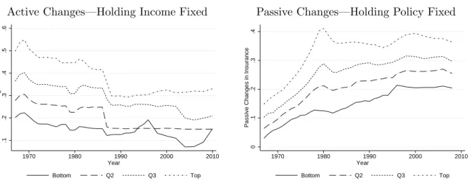
Figure 1 shows active and passive insurance changed from 1967 to 2010. As expected for a progressive tax system, the level of insurance the federal income tax provides is highest for high income taxpayers. Active insurance decreases for all income groups from 1967 to 2010, with the largest decrease occurring in 1987. This implies that observed changes in the tax code have reduced the amount of insurance provided by the federal income tax system. Passive insurance increases for all income groups from 1967 to 2010. This implies that observed changes in income distribution have led the progressive federal income tax system 19We impute income in 1980 for households that do not report income that year. Although we chose
to provide more insurance.
Figure 1: Active and Passive Insurance, by Quartiles of Income Active Changes—Holding Income Fixed
.1
.2
.3
.4
.5
.6
Active Changes in Insurance
1970 1980 1990 2000 2010 Year
Bottom Q2 Q3 Top
Passive Changes—Holding Policy Fixed
0
.1
.2
.3
.4
Passive Changes in Insurance
1970 1980 1990 2000 2010 Year
Bottom Q2 Q3 Top
NOTE.— Figure 1 shows that active changes decreased insurance and passive changes increased insurance from 1968 to 2010. Active and passive insurance changes are calculated using simulations from NBER’s TaxSim program and defined in equation (9) and (10). The income quartiles are defined in the base year 1980.
2.2.2 The Role of Federal Income Taxes on Insurance
The insurance the income tax provides depends on the nonlinear tax code and the income distribution. The change in insurance the income tax provides household i in year t due to changes in income in year t, holding fixed the nonlinear tax code to a base year, is defined as passive insurance changes Si,tP. The insurance the income tax provides individuals due to the nonlinear tax code, holding fixed a household’s income to a base year, is defined as active insurance changes SA
i,t. Together, the amount of insurance households have against
permanent income shocks is given by,
The amount of insurance households have against permanent income shocks is a function of active and passive insurance and an independent and identically distributed error term,
i,t,20
1−ψg =βgΓ(Si,tA, Si,tP) +i,t. (11)
20In our empirical estimation of these parameters, we allow for measurement error in consumption and
Totally differentiating equation (11) gives
d(1−ψg) =βgΓ0AdS
A
i,t+βgΓ0AdS P
i,t + Γ(S P i,t, S
A
i,t)dβg. (12)
The first term on the right-side of equation (12) captures changes in active insurance. The second term captures changes in passive insurance, and the third term captures all other behavioral changes in insurance due to any other factors, such as households’ propensity to consume tax rebates.21 This decomposition is similar to a Blinder-Oaxaca decomposition (Oaxaca, 1973; Blinder, 1973) widely used to analyze wage gaps by sex or race and recently used in a tax context to decompose tax revenue volatility by Seegert (2012).
2.3
Moment Conditions
This subsection derives a series of moment conditions used to estimate the variance of the permanent and transitory income shocks, the partial insurance parameters, and other model parameters such as the serial correlation of the transitory shocks. One complication of using PSID data after 1996 is that the data are only reported biannually, meaning the moment conditions based on one-year differences cannot be used. To extend our analysis to years after 1996, we construct moment conditions based on the covariances of two-year differences in income and consumption, which can be derived from the model as,
˜
∆yt=ζt+ζt−1+ ˜∆vt, and
˜
∆ct =φgζt+φgζt−1+ψεt+ψgεt−1 +ξt+ξt−1,
where ˜∆xtdefines the two-year difference in variablex.22 The first set of moment conditions
is based on the covariance of the two-year growth in income with different leads,
cov( ˜∆yt,∆˜yt+s) =
var(ζt) +var(ζt−1) +var( ˜∆vt) if s= 0
var(ζt) +cov( ˜∆vt,∆˜vt+1) if s= 1
cov( ˜∆vt,∆˜vt+2) if s= 2
, (13)
where cov(., .) and var(.) denote the cross-sectional covariance and variance, respectively. The second set of moment conditions is based on the covariance of the two-year growth in
21We allow for heterogeneity in behavioral effects by introducing group fixed effects.
22These moment conditions resemble the one-year differences used in Hall and Mishkin (1982) and Blundell,
consumption with different leads,
cov( ˜∆ct,∆˜ct+s) =
φ2gvar(ζt) +φg2var(ζt−1) +ψg2var(εt) +ψg2var(εt−1) + 2var(ξ) if s= 0
φ2gvar(ζt) +ψ2gvar(εt) +var(ξ) if s= 1
0 if s >1
.
(14) Finally, the covariance between the two-year growth in income and consumption at various lags provides the third set of moments,
cov( ˜∆yt+s,∆˜ct) =
φgvar(ζt) +φgvar(ζt−1) +ψgcov(εt,∆˜vt) +ψgcov(εt−1,∆˜vt) if s= 0
φgvar(ζt) +ψgcov(εt,∆˜vt+1) +ψgcov(εt−1,∆˜vt+1) if s= 1
ψgcov(εt,∆˜vt+2) +ψgcov(εt−1,∆˜vt+2) if s= 2
.
(15) These 252 moment conditions are used to estimate the 167 parameters from the model. The parameters of interest are the partial insurance parametersφg and ψg. Appendix C provides
more details on deriving each of the moment conditions and calculating the standard errors following Gary Chamberlain’s (1984) method.23
3
Data
To understand how income tax changes have impacted the transmission of income shocks to consumption, we need a panel database including income and consumption covering several tax regimes. We construct a database of consumption using the consumer expenditure survey (CEX) and combine it with the panel data from the Panel Study of Income Dynamics (PSID) using the imputation approach developed by Skinner (1987) and used extensively since then (Blundell and Preston, 2004; Blundell, Pistaferri, and Preston, 2008).24
One innovation of our paper is that we expand the sample years to include the years 1967 through 2010. This allows us to compare the imputed values of nondurable consumption produced through this method with data on nondurable consumption collected in the PSID from 1999 to 2010. Additional data collection information is given in Appendix A.
23The standard errors computation requires the variance-covariance matrix of the moments, the weights
used in the estimation (in this case the diagonal matrix of the inverse of the variance-covariance matrix), and the Jacobian matrix evaluated at the estimated parameters.
24Skinner (1987) imputes total consumption in the PSID using the estimated coefficients of a regression of
3.1
Sample Selection
We start with an unbalanced panel from the PSID using data from 1967 to 2010. To focus on income risk, rather than variation in consumption due to divorce, widowhood, or other household breaking-up factors, we restrict our sample to households with continuously married couples (excluding 64.2 percent of households, with or without children), headed by a male of age 30 to 65 (excluding 29.7 percent of households).25 The choice to exclude single-parent families is to ensure identification of consumption shocks stemming from income shocks rather than changes in family composition. Even among low-income households we do not think that this is an important limitation since, for example, the percentage of single and joint households receiving the EITC are similar.26
Within this sample, we create 12 cohorts, each defined as being born in a given half decade starting in 1920 and ending in 1980, eliminating 27.9 percent of the sample. Income outliers, defined as households with income growth above 500 percent, below -80 percent, or with a level of income below $100 in a given year, are eliminated (25.5 percent). We eliminate households with missing data on race (0.6 percent) and region (6.0 percent).27 Starting with 23,107 families and 243,539 observations, the final sample is composed of 4,139 households (17.9 percent) and 42,582 observations (17.5 percent). This sample selection is followed to the extent possible in the CEX. Detailed descriptions of the data collection from the PSID and CEX are given in Appendices A.4 and A.3.
An important contribution of our paper is that we allow the effect of fiscal policy to be heterogeneous, allowing different income groups to have differential access to external smoothing mechanisms in addition to self-insurance, through savings or borrowing and family networks. To this end, we use the two available samples of households in the PSID: the 25Families that report changes in head are excluded, further excluding 16.8 percent of the sample. Also,
the PSID public files do not report marital status from 1993–1996. To account for this, individuals are assigned the marital status they had in 1992 and 1997, if these two years have the same values, and dropped otherwise. This restriction also limits the changes due to changes in education and retirement.
26This sample selection also makes our paper comparable to previous studies imputing consumption from
the PSID (Blundell, Pistaferri, and Preston, 2008). We recognize that certain tax and non-tax benefits such as the EITC have largely benefited low-income single households. For instance in 2003, 76 percent of EITC recipients were single headed households. Yet,within low-income groups, the proportion of single and joint households receiving the EITC are similar. For instance in 2003, about 0.02 percent of both single-headed and joint households with less than $40,000 of AGI received the EITC (authors’ calculations using data from the Joint Committee on Taxation and SOI/IRS tax statistics). We define income groups based on 1980 income distribution, implying that intergenerational mobility likely moved low-income families in and out of the EITC over the period.
27The PSID public files do not report state for years 1993–1996. To account for this, individuals are
Table 1: Comparison of Means (Variances)—PSID and CEX
1973 1990 2010
PSID(S) PSID(R) CEX PSID(S) PSID(R) CEX PSID(S) PSID(R) CEX
Age 45.71 47.40 46.30 42.68 44.94 45.98 46.99 46.61 48.46 (9.573) (10.02) (10.20) (9.523) (10.02) (9.879) (9.991) (10.55) (10.15) Family Size 5.351 3.713 3.909 3.671 3.382 3.609 3.433 3.296 3.453
(2.571) (1.629) (1.765) (1.363) (1.206) (1.444) (1.352) (1.323) (1.449) No. of Kids 2.663 1.339 1.490 1.322 1.100 1.163 1.029 1.045 1.050
(2.210) (1.500) (1.594) (1.243) (1.184) (1.272) (1.269) (1.245) (1.241) White 0.302 0.896 0.927 0.436 0.934 0.875 0.0250 0.884 0.847
(0.460) (0.305) (0.260) (0.496) (0.248) (0.330) (0.156) (0.321) (0.360) Food expenditures 2,764 2,767 2,393 5,033 6,034 6,171 6,648 8,870 9,264
(1,286) (1,138) (973.8) (2,440) (2,718) (2,939) (4,701) (4,911) (4,526) Non-durable consumption (Imputed) 4,527 5,057 5,240 13,884 16,798 19,017 24,605 31,207 29,056 (2,701) (2,395) (2,903) (9,405) (10,519) (9,626) (29,254) (37,988) (17,279) HS dropout 0.629 0.320 0.337 0.238 0.135 0.151 0.133 0.0846 0.117
(0.484) (0.467) (0.473) (0.426) (0.342) (0.358) (0.341) (0.278) (0.321) At least some college 0.147 0.356 0.325 0.414 0.557 0.565 0.483 0.650 0.623
(0.355) (0.479) (0.469) (0.493) (0.497) (0.496) (0.501) (0.477) (0.485) Midwest 0.111 0.309 0.283 0.137 0.303 0.265 0.0958 0.292 0.251
(0.314) (0.462) (0.451) (0.344) (0.460) (0.442) (0.295) (0.455) (0.434) South 0.622 0.302 0.298 0.610 0.295 0.272 0.792 0.302 0.333
(0.486) (0.459) (0.458) (0.488) (0.456) (0.445) (0.407) (0.459) (0.472) West 0.138 0.154 0.211 0.126 0.168 0.238 0.0458 0.225 0.233
(0.345) (0.362) (0.408) (0.332) (0.374) (0.426) (0.210) (0.418) (0.423) Husband working 0.902 0.929 0.916 0.887 0.924 0.912 0.821 0.886 0.875
(0.298) (0.257) (0.277) (0.317) (0.266) (0.284) (0.384) (0.318) (0.331) Wife working 0.538 0.524 0.515 0.775 0.804 0.729 0.796 0.780 0.675
(0.499) (0.500) (0.500) (0.418) (0.397) (0.444) (0.404) (0.415) (0.468) Observations 407 693 4,283 621 851 1,301 240 981 1,767
NOTE.— R = Representative PSID households (drawn from the national survey only); S = Total PSID households (from both the representative survey and the SEO); CEX = Consumer Expenditure Survey. Standard errors are in parentheses.
representative sample of the US population and the low-income sample (SEO).28 Table 1
compares the means across the PSID SEO sample, PSID representative sample, and the CEX for the years 1973, 1990, and 2010. In all categories the demographics look very similar between the representative subsample of the PSID and the CEX. This is important for the imputation to correctly predict consumption for households in the PSID using data from the CEX.
3.2
Imputation
The imputation method relies on measures of food and nondurable consumption. Food consumption is constructed as the sum of food at home and food away from home, reported in both the PSID and CEX. In the CEX, nondurable consumption is constructed as the sum of food, alcohol, tobacco, services, heating fuel, public and private transport (including 28The PSID’s representative sample of the US population covers 61 percent of the 1967 sample and the
gasoline), personal care, clothing, and footwear, as proposed by Attanasio and Weber (1995). The PSID had limited consumption variables until additional questions were added in 1999 and 2005.29 These additional consumption data permit us to construct a PSID-based proxy
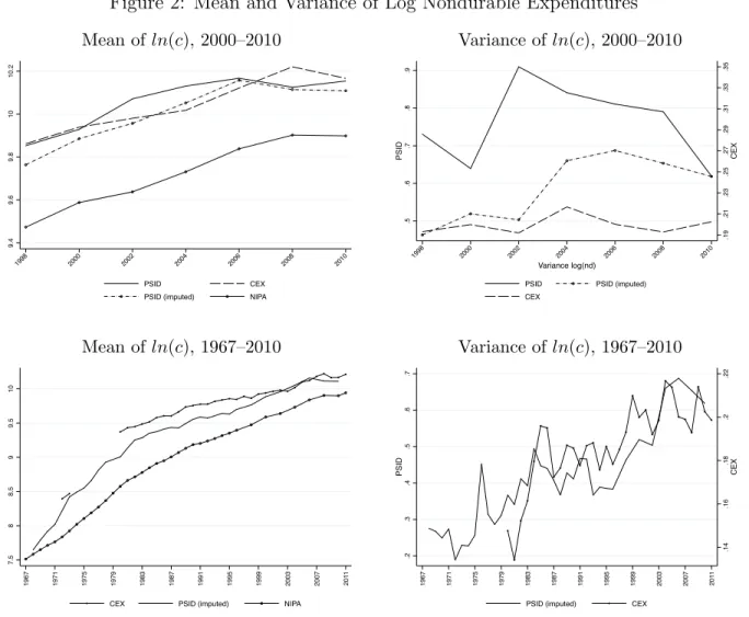
for nondurable expenditures that provide some external validity to the imputation method. These estimates are compared in Figure 2.
Although our baseline measure of consumption is nondurable consumption, we also con-sider three broader measures that alternatively include semi-durables, services from durable goods, or both, with details provided in Appendix A.3 to test the robustness of the imputa-tion and our findings.30 The imputation method uses pooled cross-sectional data from the CEX in 1972 and 1973, and from 1980 to 2010, and the following demand equation (following Blundell, Pistaferri, and Preston (2008)’s notation) for food, f, expressed in logs:
fi,t =Wi,t0 µ+p
0
tθ+β(Di,t)ci,t+ei,t, (16)
for each household i in period t with demographics, W, and relative price, p. Demand shifters controlling for nondurable expenditure are given by c, expressed in logs, and the budget elasticity β is allowed to vary with observed household characteristics, D. Finally, we allow for unobserved heterogeneity in the measurement error in food expenditures given by e. Appendix A.3 reports the results of this specification, in which we account for the measurement error in total expenditures with an instrumental variables methodology.31
Figure 2 provides external validity that the averages of imputed measures of nondurable consumption (in logs) are closely related to both the CEX and NIPA averages over time and lie consistently between the two series. Variances of imputed consumption and CEX consumption are also close throughout the period.
29Consumption variables from 1999 include healthcare expenses (e.g. hospital, doctor, and prescription
expenses), housing expenses (e.g. mortgage payments, rent, property taxes, and homeowner’s insurance), utilities, vehicle expenses (e.g. loan payments, down payments, repairs, car insurance, and gasoline costs), transportation expenses (e.g. taxi, bus, and train), education expenses, and adult care expenses. Additional consumption variables added in 2005 include cell phone, internet, and cable expenses, recreation and vacation expenses, furnishings, clothing, home repair, and charitable giving.
30Consumers also use durable goods to smooth non-durable consumption, implying that total consumption
including durables is more volatile over the life cycle. Yet, if the imputation method and the model are correct, our estimates of the impact of tax policy on insurance should not be affected by the inclusion of durable goods.
31To provide further external validity to the imputed values they are compared with reported nondurable
Figure 2: Mean and Variance of Log Nondurable Expenditures Mean of ln(c), 2000–2010
9.4
9.6
9.8
10
10.2
1998 2000 2002 2004 2006 2008 2010
PSID CEX
PSID (imputed) NIPA
Variance ofln(c), 2000–2010
.19 .21 .23 .25 .27 .29 .31 .33 .35 C EX .5 .6 .7 .8 .9 PSI D
1998 2000 2002 2004 2006 2008 2010
Variance log(nd)
PSID PSID (imputed)
CEX
Mean of ln(c), 1967–2010
7.5 8 8.5 9 9.5 10
1967 1971 1975 1979 1983 1987 1991 1995 1999 2003 2007 201
1
CEX PSID (imputed) NIPA
Variance ofln(c), 1967–2010
.14 .16 .18 .2 .22 C EX .2 .3 .4 .5 .6 .7 PSI D
1967 1971 1975 1979 1983 1987 1991 1995 1999 2003 2007 201
1
PSID (imputed) CEX
NOTE.— See Table A.2 notes for an explanation of the NIPA average and nondurable consumption impu-tation (PSID imp.).
4
Empirical Evidence
the impact on this insurance of active and passive tax policy changes from 1968 to 2010 observed from the decomposition defined in section 2.2.2.
4.1
The Autocovariance of Income and Consumption Growth
Figure 3 shows that income inequality increased from 1967 to 2010, measured as the variance of income growth. The variance of income growth experienced increases in the mid-1980s and a prolonged increase in the 1990s. Panel B of Figure 3 shows that consumption inequal-ity increased from 1967 to 2010, measured as the variance of consumption growth.32 The
variance of consumption growth experienced increases from the mid-1970s through the 1980s and again in the 2000s.33 The different timing of the increases in inequality stems from both
differences in the nature of the income shocks (permanent or transitory) and differences in the transmission of income shocks to consumption.
Figure 3: Variance of Income and Consumption Growth— 1967 to 2010 Income
.05
.1
.15
.2
1967 1971 1975 1979 1983 1987 1991 1995 1999 2003 2007 201
1
Income
Standard Two-yr
Consumption
0
.2
.4
.6
1967 1971 1975 1979 1983 1987 1991 1995 1999 2003 2007 201
1
Consumption
Standard Two-yr
NOTE.— Figure 3 shows the increase in income and consumption inequality from 1967–2010. Estimates, with standard errors, are reported in Tables E.1 and E.2.
Figure 4 shows the contemporary covariance of consumption and income growth by in-come quartiles. The covariance of consumption and inin-come is a key variable in the identi-fication of the insurance parameters. In the extreme case of full insurance, the covariance 32The variance of consumption growth also captures the heterogeneity in household’s responses to income
shocks and the measurement error from the imputation.
33Estimated values of these variances as well as their autocovariances and their standard errors are reported
would be zero. Deviations of this covariance from zero inform about changes in the insurance parameters.
The contemporary covariance of consumption and income is larger in the period 1980– 1992 period than in the periods 1967–1979 and 1993–2010. These differences across periods suggest lower insurance from income shocks during 1980–1992 than during 1967–1979 and 1993–2010.
Figure 4: Contemporary Covariances of Consumption and Income Growth, By Quartile Of Income Q1 (Bottom) -. 0 5 -. 0 3 -. 0 1 .01 .03 .05 .07 .09
1967 1971 1975 1979 1983 1987 1991 1995 1999 2003 2007 201
1 Standard Two-yr Q2 -. 0 5 -. 0 3 -. 0 1 .01 .03 .05 .07 .09
1967 1971 1975 1979 1983 1987 1991 1995 1999 2003 2007 201
1 Standard Two-yr Q3 -. 0 5 -. 0 3 -. 0 1 .01 .03 .05 .07 .09
1967 1971 1975 1979 1983 1987 1991 1995 1999 2003 2007 201
1 Standard Two-yr Q4 (Top) -. 0 5 -. 0 3 -. 0 1 .01 .03 .05 .07 .09
1967 1971 1975 1979 1983 1987 1991 1995 1999 2003 2007 201
1
Standard Two-yr
4.2
Variance of Permanent and Transitory Income Shocks
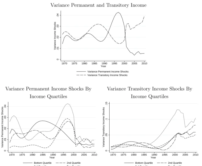
Figure 5 depicts a nonparametric estimate of the trends in the variances of permanent and transitory income shocks from 1968 to 2010. These estimates provide four types of evidence. First, we provide evidence on whether the increase in consumption inequality is due to permanent or transitory income shocks. Figure 5 shows that the variance of permanent income shocks increased in the early 1980s and late 1990s. The variance of transitory in-come shocks increased in the early and middle 1980s and in the 2000s. This suggests that changes in the variance permanent and transitory income shocks contributed to the increase in consumption inequality but at different times.
Second, the partial insurance parameter estimates (reported below in section 4.3) are identified by moment conditions that combine the variance of consumption growth and the variance of permanent and transitory income shocks. This suggests that we can anticipate the partial insurance estimates by comparing the variance of consumption growth and per-manent and transitory income shocks. For example, consider our findings that the variance of permanent income shocks increased in the 1990s (Figure 5) but the variance of consump-tion growth did not (Figure 3). This suggests that insurance to permanent income shocks must have increased in the 1990s to damp the transmission of permanent income shocks to consumption. As another example, consider our findings that the variance of transitory in-come shocks and the variance of consumption growth increased in the 2000s (Figures 5 and 3 respectively). This suggests that insurance to transitory income shocks may have decreased in the 2000s, allowing the increase in transitory income shocks to impact consumption.
Figure 5: Variance of Permanent and Transitory Income Shocks
Variance Permanent and Transitory Income
0
.01
.02
.03
.04
Variance Income Shocks
1970 1975 1980 1985 1990 1995 2000 2005 2010 Year
Variance Permanent Income Shocks Variance Transitory Income Shocks
Variance Permanent Income Shocks By Income Quartiles
0
.01
.02
.03
.04
Variance Permanent Income Shocks
1970 1975 1980 1985 1990 1995 2000 2005 2010 Year
Bottom Quartile 2nd Quartile 3rd Quartile Top Quartile
Variance Transitory Income Shocks By Income Quartiles
0
.05
.1
.15
Variance Transitory Income Shocks
1970 1975 1980 1985 1990 1995 2000 2005 2010 Year
Bottom Quartile 2nd Quartile 3rd Quartile Top Quartile
NOTE.— The trends are nonparametric estimates of a flexible trend. Figure E.3 finds the baseline trends in the estimates of the variance of permanent and transitory income shocks (reported in this figure) are similar to those using the method from Kopczuk, Saez, and Song (2010).
4.3
Partial Insurance: the Transmission of Income Shocks to
Con-sumption
comparisons of our estimates to other studies. The larger the partial insurance parameter (the closer to 1), the larger the fraction of households’ income shocks that transfers to consumption (i.e., the smaller the amount of insurance). We further investigate differences in partial insurance parameters across income quartiles.
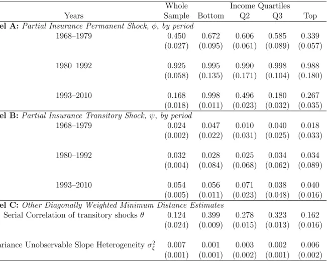
4.3.1 Partial Insurance Estimates
Table 2 reports the diagonally weighted minimum distance estimates. Panel A reports the partial insurance parameter to permanent income shocks was the highest in the period 1980– 1992 and the lowest in 1993–2010. This is consistent with the suggestive evidence from the autocovariance of income and consumption of a the relatively flat variance of consumption growth in the 1990s (Figures 3 and 4), and the increase in the variance of permanent income shocks in the 1990s.34 We observe the same general pattern of an increase in the transmission
of permanent income shocks to consumption from 1968–1979 to 1980–1992 followed by a subsequent decrease in 1993–2010 for all income quartiles (columns 2-4), except that the bottom income quartile does not experience the subsequent decrease in 1993–2010. This evidence suggests that the decrease in insurance to permanent income shocks in 1980–1992 contributed to the increase in consumption inequality in the 1980s.
Panel B reports the partial insurance parameter of transitory income shocks is an order of magnitude smaller than the partial insurance parameter of permanent income shocks. This suggests that households smooth consumption more relative to a transitory income shock than a permanent income shock. The partial insurance parameter of transitory in-come shocks increased from 0.024 in 1968–1979 to 0.054 in 1993-2010. The increase in the transmission of transitory income shocks to consumption is consistent with the evidence that both the variances of transitory income shocks and consumption growth increased in the 2000s (Figures 3 and 5). This evidence suggests that the decrease in insurance to tran-sitory income shocks in 1993–2010 contributed to the increase in consumption inequality in the 2000s.
Panel C reports the serial correlation parameter and the variance of unobservable slope heterogeneity. These estimates provide a check on external validity. If our model and estimation are fitting the data, then we’d expect our estimates to be similar to those in other studies. Our estimate of the serial correlation parameter is 0.124, which is similar to 34Kniesner and Ziliak (2002) use a similar semi-parametric decomposition of income shocks’ variance into
the 0.113 estimate in Blundell, Pistaferri, and Preston (2008). Our estimate of the variance of unobservable slope heterogeneity is 0.007, which is similar to the 0.010 estimate in Blundell, Pistaferri, and Preston (2008). The similarity in estimates suggests our model and estimation are fitting the data.
The standard errors in Table 2 are calculated using Gary Chamberlian’s (1984) method and reported in parentheses.35
4.3.2 Active and Passive Insurance Impacts
This section reports the level and change in total insurance, (1−φ) and (1−ψ), and the level and change in insurance if only active or passive changes in insurance would have occurred. These estimates are calculated from the decomposition presented in equation (12) with bootstrapped standard errors reported in parentheses. For brevity, we report only the estimates for the whole sample, with more detailed estimates by income quartile reported in Appendix E. 3.36 These estimates provide a baseline understanding of the ability of active
and passive tax policy changes to damp income inequality.
For convenience, Table 3 reports changes in insurance, that is (1−φ) in equation (12), rather than the partial insurance coefficient (φ). Panel A reports the insurance to permanent income shocks and Panel B reports the insurance to transitory income shocks. The first two columns report the level and change in total insurance, obtained from the estimates of φ
and ψ reported in Table 2. Columns 3–6 report the extent these changes are attributable to active and passive tax policy changes.
Columns 3 and 4 report that active tax policy changes led to a 45 percent decrease in insurance to permanent income shocks and a 24 percent decrease to insurance to transitory income shocks. Panel A reports a level decrease in the insurance to permanent income shocks of 0.026 between the first two periods and 0.223 between the last two periods. Panel B reports a level decrease in the insurance to transitory income shocks of 0.059 between the first two periods and 0.177 between the last two periods. These results suggest that changes in the tax structure decreased insurance and increased the transmission of income shocks 35Gary Chamberlian shows that the variance of the parameters can be estimated according to the equation
\
var( ˆΛ) = (G0AG)−1G0AV AG(G0AG)−1,whereGis the Jacobian matrix evaluated at the estimated
param-eters ˆΛ and A is a weighting matrix equal to diag(V−1) for our diagonally weighted minimum distance
estimates.
36Our findings add to the evidence that tax policy is an important factor for income and consumption
Table 2: Diagonally Weighted Minimum Distance Estimates
Whole Income Quartiles
Years Sample Bottom Q2 Q3 Top
Panel A:Partial Insurance Permanent Shock,φ, by period
1968–1979 0.450 0.672 0.606 0.585 0.339
(0.027) (0.095) (0.061) (0.089) (0.057)
1980–1992 0.925 0.995 0.990 0.998 0.988
(0.058) (0.135) (0.171) (0.104) (0.180)
1993–2010 0.168 0.998 0.496 0.180 0.267
(0.018) (0.011) (0.023) (0.032) (0.035)
Panel B:Partial Insurance Transitory Shock,ψ, by period
1968–1979 0.024 0.047 0.010 0.040 0.018
(0.002) (0.022) (0.031) (0.025) (0.033)
1980–1992 0.032 0.028 0.025 0.034 0.034
(0.004) (0.084) (0.068) (0.062) (0.089)
1993–2010 0.054 0.056 0.071 0.038 0.040
(0.005) (0.011) (0.023) (0.048) (0.016)
Panel C:Other Diagonally Weighted Minimum Distance Estimates
Serial Correlation of transitory shocksθ 0.124 0.399 0.278 0.323 0.162
(0.024) (0.009) (0.015) (0.013) (0.016)
Variance Unobservable Slope Heterogeneityσ2
ξ 0.007 0.001 0.003 0.002 0.006
(0.001) (0.001) (0.002) (0.001) (0.002)
to consumption. Said differently, active changes from 1968 to 2010 increased consumption inequality.
Columns 5 and 6 report that passive tax policy changes led to a 32 percent increase in insurance to permanent income shocks and a 16 percent increase to insurance to transitory income shocks. Panel A reports a level increase in the insurance to permanent income shocks of 0.025 between the first two periods and 0.154 between the last two periods. Panel B reports a level increase in the insurance to transitory income shocks of 0.05 between the first two periods and 0.109 between the last two periods. These results suggest that the nonlinear structure of the personal income tax interacted with changes in the income distribution in a way that increased insurance to permanent and transitory income shocks. Said differently, passive changes from 1968 to 2010 damped consumption inequality.
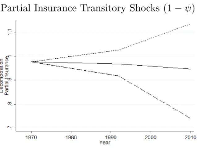
Figure 6 shows the overall change in insurance and the changes due to active and passive tax policy changes. All other changes in insurance, for example, due to changes in credit availability, is given by the difference between the overall change in insurance and the net change due to active and passive tax policy changes. Figure 6 shows that despite the large impact active and passive tax policy changes had on insurance, their impacts offset each other overall—motivating the importance of separating these two mechanisms. This explains why despite large changes in tax policy that led to large changes in disposable income, previous studies have not found a large impact of tax policy changes on the transmission of income shocks to consumption.
Table 3: Active and Passive Changes to Partial Insurance
Total Active Passive Level Change Level Change Level Change
Panel A:Partial Insurance Permanent Shock,(1−φ),by period
1968–1979 0.550 0.550 0.550 (0.027) (0.027) (0.027) 1980–1992 0.075 −0.475 0.523 −0.026 0.574 0.025
(0.058) (0.075) (0.001) (0.001) (0.002) (0.002) 1993–2010 0.832 0.757 0.300 −0.223 0.728 0.154
(0.018) (0.067) (0.006) (0.006) (0.005) (0.005)
Panel B:Partial Insurance Transitory Shock,(1−ψ),by period
1968–1979 0.976 0.976 0.976 (0.002) (0.002) (0.002) 1980–1992 0.968 0.008 0.917 −0.059 1.026 0.050
(0.004) (0.003) (0.009) (0.009) (0.005) (0.005) 1993–2010 0.946 0.022 0.740 −0.177 1.135 0.109
(0.005) (0.006) (0.019) (0.021) (0.024) (0.026)
Figure 6: Changes In Partial Insurance Permanent and Transitory Shocks, (1−φ) and (1−ψ) Partial Insurance Permanent Shocks (1−φ) Partial Insurance Transitory Shocks (1−ψ)
5
Conclusion
The federal income tax can affect the economy in several ways, including income and con-sumption inequality. This paper identifies and estimates the effects of two mechanisms by which the federal income tax affected consumption inequality between 1968 to 2010. We define changes in insurance due to changes in tax policy asactive changes in insurance. We define changes in insurance due to the interaction between changes in the income distri-bution and the nonlinear income tax schedule as passive changes in insurance. Separately identifying the impact of active and passive tax policy changes on insurance allows us to provide evidence on how tax policy changes impacted the transmission of income shocks to consumption.
We find that active tax policy changes between 1968 and 2010 decreased insurance to permanent income shocks by 45 percent and decreased insurance to transitory income shocks by 24 percent. Said differently, consumption inequality would have been substantially smaller during this period if tax policy had not changed between 1967 and 2010. This implies that tax policy is an important instrument to combat consumption inequality.
policy is a poor instrument for addressing consumption inequality.
References
Abowd, J. M., and D. Card (1989): “On the Covariance Structure of Earnings and
Hours Changes,” Econometrica, 57(2), 411–45.
Aguiar, M. A., and M. Bils (2011): “Has Consumption Inequality Mirrored Income
Inequality?,”NBER Working Paper, (16807).
Altonji, J. G., and A. Siow (1987): “Testing the response of consumption to income
changes with (noisy) panel data,”The Quarterly Journal of Economics, 102(2), 293–328.
Alvarez, F., and U. J. Jermann (2000): “Efficiency, Equilibrium, and Asset Pricing
with Risk of Default,” Econometrica, 68(4), 775–98.
Attanasio, Orazio P., E. H., and L. Pistaferri (2012): “The Evolution of
In-come, Consumption, and Leisure inequality in the US, 1980-2010,”NBER Working Paper, (17982).
Attanasio, O. P., and G. Weber (1995): “Is Consumption Growth Consistent with
Intertemporal Optimization? Evidence from the Consumer Expenditure Survey,”Journal of Political Economy, 103(6), 1121–57.
Auerbach, A. J., and D. Feenberg (2000): “The significance of federal taxes as
auto-matic stabilizers,”Journal of Economic Perspectives, 14(3), 37–56.
Autor, David H., L. F. K., andM. S. Kearney(2008): “Trends in US wage inequality:
Revising the revisionists,”The Review of Economics and Statistics, 90(2), 300–323.
Bargain, Olivier, M. D. H. I. D. N. A. P. N. P., and S. Siegloch (2014): “Tax
policy and income inequality in the US, 1979-2007,”Economic Inquiry, 53(2), 1061–85.
Blinder, A. S. (1973): “Wage discrimination: reduced form and structural estimates,”
Journal of Human Resources, pp. 436–55.
Blundell, Richard, H. L., and I. Preston (2013): “Decomposing changes in income
risk using consumption data,”Quantitative Economics, 4, 1–37.
Blundell, Richard, L. P. L., and I. Preston (2004): “Imputing consumption in the
PSID using food demand estimates from the CEX,”Institute for Fiscal Studies Working Paper, (04/27).
Blundell, R.,and L. Pistaferri(2003): “Income volatility and household consumption:
The impact of food assistance programs,” Journal of Human Resources, 38(S), 1032–50.
Blundell, R., L. Pistaferri, and I. Preston (2008): “Consumption inequality and
Bound, J., and A. B. Krueger(1991): “The Extent of Measurement Error in
Longitu-dinal Earnings Data: Do Two Wrongs Make a Right?,”Journal of Labor Economics, 9(1), 1–24.
Butrica, B. A., and R. V. Burkhauser (1997): “Estimating federal income tax
bur-dens for Panel Study of Income Dynamics (PSID) families using the National Bureau of Economic Research Taxsim model,” Maxwell Center for Demography and Economics of Aging, Paper No.12.
Caballero, R. J. (1990): “Consumption puzzles and precautionary savings,” Journal of
Monetary Economics, 25(1), 113–36.
Carroll, C. D. (2001): “Precautionary saving and the marginal propensity to consume
out of permanent income,” NBER Working Paper, (8233).
(2009): “Precautionary saving and the marginal propensity to consume out of permanent income,” Journal of Monetary Economics, 56(6), 780–90.
Carroll, C. D., and M. S. Kimball(2001): “Liquidity Constraints and Precautionary
Saving,” NBER Working Paper, (8496).
Cutler, D. M., and L. F. Katz(1992): “Rising Inequality? Changes in the Distribution
of Income and Consumption in the 1980’s,”American Economic Review, 82(2), 546–51.
Danziger, Sheldon, J. V. d. G., and E. Smolensky (1984): “Income Transfers and
the Economic Status of the Elderly,” in Economic Transfers in the United States, ed. by M. Moon, pp. 239 – 82. University of Chicago Press.
Deaton, A. (1991): “Saving and liquidity constraints,” Econometrica, 59(5), 1221–48.
Debacker, Jason, B. H. V. P. S. R., and I. Vidangos (2013): “Rising inequality:
Transitory or persistent? New evidence from a panel of US tax returns,”Brookings Papers on Economic Activity, pp. 67–122.
Dolls, Mathias, C. F., and A. Peichl (2012): “Automatic stabilizers and economic
crisis: Us vs. Europe,”Journal of Public Economics, 96(3-4), 27994.
Gillingham, R., and J. S. Greenlees (1990): “Indexing the Federal Tax System: a
cost-of-living approach,”Journal of Business & Economic Statistics, 8(4), 465–473.
Gottschalk, P., and R. A. Moffitt (2009): “The rising instability of US earnings,”
The Journal of Economic Perspectives, pp. 3–24.
Gottschalk, P., and T. M. Smeeding (1997): “Cross-national comparisons of earnings
and income inequality,” Journal of economic literature, pp. 633–687.
Guvenen, F. (2007): “Learning your earning: are labor income shocks really very
Hall, R. (1978): “Stochastic implications of the life cycle-permanent income hypothesis:
Theory and evidence,”Journal of Political Economy, 86(6), 97187.
Hall, R., and F. Mishkin (1982): “The sensitivity of consumption to transitory income:
Estimates from panel data of households,” Econometrica, 50(2), 261–81.
Heathcote, Jonathan, F. P., and G. L. Violante (2010): “Unequal we stand: An
empirical analysis of economic inequality in the United States, 1967–2006,” Review of Economic Dynamics, 13(1), 15–51.
Johnson, David S., T. M. S.,and B. B. Torrey(2005): “Economic inequality through
the prisms of income and consumption,”Monthly Labor Review.
Kniesner, T. J., and J. P. Ziliak (2002): “Tax reform and automatic stabilization,”
The American Economic Review, 92(3), 590–612.
Kopczuk, Wojciech, E. S., and J. Song (2010): “Earnings inequality and mobility in
the United States: evidence from social security data since 1937,”The Quarterly Journal of Economics, 125(1), 91–128.
Krueger, D., and F. Perri (2005): “Does income inequality lead to consumption
in-equality? Evidence and theory,” Federal Reserve Bank of Minneapolis, (Research Staff Report 363).
(2006): “Does income inequality lead to consumption inequality? Evidence and theory,” The Review of Economic Studies, 73(1), 163–193.
Ludvigson, S., and C. H. Paxson(2001): “Approximation bias in linearized Euler
equal-tions,”Review of Economics and Statistics, 83(2), 242–56.
MaCurdy, T. E. (1982): “The use of time series processes to model the error structure of
earnings in a longitudinal data analysis,”Journal of Econometrics, 18(1), 83–114.
Meghir, C., and L. Pistaferri(2004): “Income Variance Dynamics and Heterogeneity,”
Econometrica, 72(1), 1–32.
Moffitt, R. A., and P. Gottschalk (2002): “Trends in the transitory variance of
earnings in the United States,”The Economic Journal, 112(478), C68–C73.
(2011): “Trends in the covariance structure of earnings in the U.S.: 1969-1987,” Journal of Economic Inequality, 9(3), 439–59.
(2012): “Trends in the transitory variance of male earnings: Methods and evidence,” The Journal of Human Resources, 47(1), 204–36.
Oaxaca, R. L. (1973): “Male-female wage differentials in urban labor markets,”
P., A. O., and N. Pavoni (2011): “Risk Sharing in Private Information Models With
Asset Accumulation: Explaining the Excess Smoothness of Consumption,”Econometrica, 79(4), 1027–1068.
Pechman, J. A.(1973): “Responsiveness of the Federal Individual Income Tax to Changes
in Income,” Brookings Papers on Economic Activity, 4(2), 385–428.
Piketty, T., and E. Saez (2007): “How Progressive is the U.S. Federal Tax System? A
Historical and International Perspective,”Journal of Economic Perspectives, 21(1).
Primiceri, G. E., and T. V. Rens(2009): “Heterogeneous life-cycle profiles, income risk
and consumption inequality,” Journal of Monetary Economics, 56(1), 20–39.
Seegert, N.(2012): “Optimal taxation with volatility: A theoretical and empirical
decom-position,”Job Market Paper, University of Michigan.
Skinner, J. (1987): “A superior measure of consumption from the panel study of income
dynamics,” Economic Letters, 23(2), 213–16.
Slesnick, D. T. (1994): “Consumption, Needs and Inequality,” International Economic
Review, 35(3).
Storesletten, Kjetil, C. I. T.,andA. Yaron(2004a): “Consumption and risk sharing
over the life cycle,”Journal of Monetary Economics, 51(3), 609–633.
(2004b): “Cyclical Dynamics in Idiosyncratic Labor Market Risk,” Journal of Political Economy, 112(3), 695–717.
Violante, G. L. (2002): “Technological Acceleration, Skill Transferability, and the Rise
in Residual Inequality,” The Quarterly Journal of Economics, 117(1), 297–38.
Zeldes, S. P. (1989): “Consumption and Liquidity Constraints: An Empirical
Investiga-tion,”Journal of Political Economy, 97(2), 305–46.
Ziliak, J. P. (1998): “Does the Choice of Consumption Measure Matter? An Application
to the Permanent Income Hypothesis,”Journal of Monetary Economics, 41(1), 20116.
Ziliak, J. P., andT. J. Kniesner(2005): “The effect of income taxation on consumption
APPENDIX FOR ONLINE PUBLICATION
Appendix A
Data
A.1
Imputation of Nondurable Expenditures
The imputation method relies on measures of food and nondurable consumption. Food consumption is constructed as the sum of food at home and away from home, reported in both the PSID and CEX. Our baseline and preferred measure of nondurable consumption is constructed from the CEX as the sum of food, alcohol, tobacco, services, heating fuel, public and private transport (including gasoline), personal care, clothing, and footwear, as proposed by Attanasio and Weber (1995). Although the PSID had limited consumption variables until additional questions were added in 1999 and 2005, we use these additional data to construct a measure of consumption that we use as a gauge for the the quality of our imputed values of nondurables, aimed to provide some external validity to the imputation method.37
The imputation method uses pooled cross-section data from the CEX in 1972 and 1973 and from 1980 to 2008 and the following demand equation (following Blundell, Pistaferri, and Preston (2008)’s notation) for food, f, expressed in logs:
fi,t =Wi,t0 µ+p
0
tθ+β(Di,t)ci,t+ei,t, (A.1)
whereW includes demographics for each householdiin periodt, andpdenotes relative prices of goods obtained from the Bureau of Labor Statistics’ series of the CPI index components (All Urban Consumers). Demand shifters controlling for nondurable expenditure are given byc, expressed in logs, and the budget elasticityβ is allowed to vary with observed household characteristics, D. Finally, we allow for unobserved heterogeneity in the measurement error in food expenditures given by e.
Table A.1 reports the results of a 2SLS of equation (A.1), where we instrument for total expenditures to account for measurement error. Instruments include average hourly wages of husbands and wives by year, number of kids, and education. External instruments include demographics such as age, ethnicity, region, family size, and cohorts. This specification passes the test of over-identifying restrictions, as the test fails to reject the null hypothesis that instrumental variables are uncorrelated with the residuals (p-value of 18.7 percent).38
The estimates generally have the expected sign and magnitude. The price elasticity is -0.93, 37Consumption variables from 1999 include healthcare expenses (e.g., hospital, doctor, and prescription
expenses), housing expenses (e.g., mortgage payments, rent, property taxes, and homeowner’s insurance), utilities, vehicle expenses (e.g., loan payments, down payments, repairs, car insurance, and gasoline costs), transportation expenses (e.g., taxi, bus, and train), education expenses, and adult care expenses. Additional consumption variables added in 2005 include cell phone, internet, and cable expenses, recreation and vacation expenses, furnishings, clothing, home repair, and charitable giving.


![Studi Perbanyakan Vegetatif Tanaman Taka (Tacca Leontopetaloides (L.) Kuntze) Dan Pola Pertumbuhannya [Study on Vegetative Propagation of Polynesian Arrowroot (Tacca Leontopetaloides) and Its Growth Pattern]](data:image/gif;base64,R0lGODlhAQABAIAAAP///wAAACH5BAEAAAAALAAAAAABAAEAAAICRAEAOw==)