Chapter 10
Thermodynamic Curvature and Black Holes
George Ruppeiner
In my talk, I will discuss black hole thermodynamics, particularly what happens when you add thermodynamic curvature to the mix. Although black hole thermodynamics is a little off the main theme of this workshop, I hope nevertheless that my message will be of some interest to researchers in supersymmetry and supergravity. Black hole thermodynamics would appear very much in need of some microscopic foundation. We might ask: what are black holes made out of? I will give no answer, but I would like to suggest that what I present here might offer some guidance about the microscopic character of black holes.
Thermodynamic curvature is an element of thermodynamic metric geometry. A pioneering paper on this was by Weinhold [1] who introduced a thermodynamic energy inner product. This led to the work of Ruppeiner [2] who wrote a Riemannian thermodynamic entropy metric to represent thermodynamic fluctuation theory, and was the first to systematically calculate the thermodynamic Ricci curvature scalar R. A parallel effort was by Andresen et al. [3] who began the systematic applica-tion of the thermodynamic entropy metric to characterize finite time thermodynamic processes.
This talk presents a review of thermodynamic curvature R broad in scope, though far from complete in its coverage. I extend the themes discussed in a previous talk [4]. My main focus is on achieving some understanding of thermodynamic curvature in the black hole setting. To accomplish this, my working assumption is that for black holes, R follows the same physical interpretation as for ordinary thermodynamic systems, where R gives the size of organized microscopic structures. I present a review of what is known about ordinary thermodynamics, and what this might tell us about black holes.
G. Ruppeiner (
B
)Division of Natural Sciences, New College of Florida, Sarasota, FL 34243-2109, USA e-mail: [email protected]
S. Bellucci (ed.), Breaking of Supersymmetry and Ultraviolet Divergences 179
in Extended Supergravity, Springer Proceedings in Physics 153,
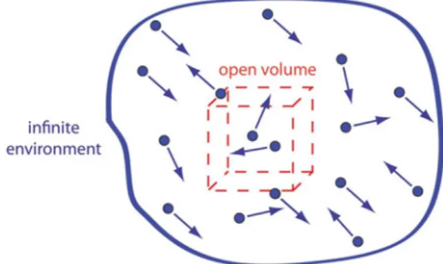
Fig. 10.1 An infinite
environ-ment of particles and an open volume, with fixed volume V , into which particles fluctuate in and out
10.1 What is Thermodynamic Curvature R?
Thermodynamic curvature comes from thermodynamic fluctuation theory. This clas-sical theory is described in every book on statistical mechanics; it is chapter twelve in Landau and Lifshitz [5]. For a fluid system, the basic set-up is shown in Fig.10.1. There is a infinite universe of particles and some imaginary open volume with fixed volume V , into which the particles can travel freely in and out. What is the probabil-ity of finding some energy U and some number of particles N in the open volume? Thermodynamic fluctuation theory gives the answer.
Let the particles in the open volume, and the environment consisting of the rest of the particles, be two thermodynamic systems. Denote the fixed thermodynamic state of the environment by “0”. The thermodynamic state of the open volume fluctuates about an equilibrium characterized by maximum total entropy. The probability of a fluctuation away from equilibrium is given by Einstein’s famous Gaussian thermo-dynamic fluctuation formula [5–8]:
probability∝exp
−V
2(Δ)
2
, (10.1)
where
(Δ)2=g
μνΔxμΔxν, (10.2)
x1 and x2 denote a pair of independent fluctuating thermodynamic variables of the open volume, Δxα = xα−xα0denotes the difference between xα and its equilibrium value x0α, where the total entropy is maximized, and gμν denotes the elements of the thermodynamic entropy metric discussed below.
gαβ= − 1
kBV
∂2S
∂Xα∂Xβ, (10.3)
where kB is Boltzmann’s constant [5,9,10]. Since probability depends only on the
thermodynamic state, the metric elementsgαβconstitute a second-rank tensor.gαβ
is a positive definite matrix, since the entropy has a maximum value in equilibrium. This is the condition of thermodynamic stability.
This is all found in Landau and Lifshitz [5]. Let me now get into some things Landau and Lifshitz did not say. The quadratic form(Δ)2in (10.2) has the look of a distance between thermodynamic states, a distance in the form of a Riemannian metric. The physical interpretation is that: the less the probability of a fluctuation between two states, the further apart they are.
A Riemannian metric in any context leads directly to a Ricci curvature scalar R [11], and this is certainly the case here. R is the only geometric scalar invariant function in thermodynamics, and so it must be very fundamental. The units of the thermodynamic curvature are those of volume per particle, and this limits its pos-sible physical interpretation greatly. Units alone suggest that R is a measure of the characteristic size of some sort of organized fluctuating structures within the system. R is readily calculable from the thermodynamic metric elementsgαβ. For exam-ple, inx1,x2=(T,ρ)coordinates, where T is the temperature andρis the particle number density, we have the Helmholtz free energy per volume f = f(T,ρ), the entropy per volume s= −f,T (where the comma notation indicates partial
differen-tiation), and the chemical potentialμ= f,ρ. The diagonal metric elements (g12 =0)
are [12]
g11 =
1 kBT
∂ s
∂T
ρ, (10.4)
and
g22 =
1 kBT
∂μ
∂ρ
T
. (10.5)
For a diagonal metric [11]
R= √1g ∂
∂x1
1
√g∂g∂ 22
x1 +∂∂ x2 1
√g∂g∂ 11
x2
, (10.6)
where
g=g11g22. (10.7)
A simple example is the ideal gas, in which there is no interaction between the particles. Here
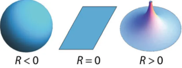
Fig. 10.2 Three surfaces with constant Ricci curvature scalar R the sphere, the plane, and the pseudosphere. For pure fluids, in Weinberg’s sign convention, R < 0 if attractive interparticle interactions dominate, and R>0 if repulsive interactions dominate. Regardless the sign convention for R, attractive interactions correspond to the geometry of the sphere, and repulsive interactions to the geometry of the pseudosphere
where h(T)is some function of the temperature with negative second derivative. Equation (10.6) now yields R=0 [2]. This suggests that R is some type of measure of interactions between particles.
Calculations in critical point models show that|R|diverges as the correlation volumeξd, where d is the spatial dimension of the system [2,9,13]. The connection of|R|to fluctuating structure size has also been established directly by means of a covariant thermodynamic fluctuation theory [9,12,14–16].
R is a signed quantity, as shown in Fig.10.2. I use the sign convention of Weinberg [17]. (Sign conventions differ among authors. I express all results reported here in Weinberg’s sign convention). For fluid and solid systems, an overall pattern is that R is negative for systems where attractive interparticle interactions dominate, and positive where repulsive interactions dominate. The sign of R alone thus offers direct information about the character of the interactions among the particles.
10.2 R for Ordinary Thermodynamics
R has been worked out in a number of cases in ordinary thermodynamics. On sys-tematic tabulation, patterns readily become evident. Such patterns might lend insight into the nature of black hole microscopic properties.
In this section I attempt a classification of the “basic food groups” of R for ordi-nary thermodynamics. Thermodynamics divides neatly into atomic and molecular systems, like fluids and solids, and discrete lattice systems, like magnetic spin sys-tems. I will treat them separately.
10.2.1 R for Fluid and Solid Systems, Basic Models
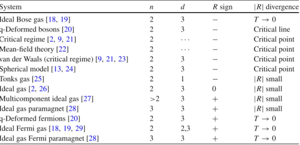
Table 10.1 The thermodynamic curvature R for a number of simple models for which R has only
one sign
System n d R sign |R|divergence
Ideal Bose gas [18,19] 2 3 − T →0 q-Deformed bosons [20] 2 3 − Critical line Critical regime [2,9,21] 2 · · · − Critical point Mean-field theory [22] 2 · · · − Critical point van der Waals (critical regime) [9,21,23] 2 3 − Critical point Spherical model [13,24] 2 3 − Critical point
Tonks gas [25] 2 1 − |R|small
Ideal gas [2,26] 2 3 0 |R|small
Multicomponent ideal gas [27] >2 3 + |R|small Ideal gas paramagnet [28] 3 3 + |R|small q-Deformed fermions [20] 2 3 + T →0 Ideal Fermi gas [18,19,29] 2 2,3 + T →0 Ideal gas Fermi paramagnet [28] 3 3 + T →0 Tabulated are the number of independent thermodynamic parameters n, the spatial dimension d, the sign of R, and the possible divergences of R. For some models, there is no particular spatial dimension d, and this is denoted by. . .. “|R|small” means that the value of|R|is on the order of the volume of an interparticle spacing or less
Table10.1shows R for a number of simple models for which R has only one sign. These models were worked out by a number of authors over a period of years. In these models interactions between particles may take place by virtue of a potential between the particles, or through quantum statistics. In either case, particles tend to either bunch together (attract) or to push apart (repel) compared with the ideal gas. The results in Table 10.1clearly show the relation between the character of the interparticle interactions and the sign of R. If interactions between particles are attractive, R is negative. Prominent here is the ideal Bose gas,1and the typical critical point models. If interactions are repulsive, R is positive. Prominent examples are ideal Fermi gasses. In systems with weak interactions, |R|is zero or “small,” where “small” means on the order of the molecular volumev,|R| ∼ vor smaller. Cases with|R| ∼ v are typical also of systems dominated by strong short-range repulsive interactions, such as dense liquids and solids. Table10.1also shows where
|R|diverges, typically either at absolute zero or at critical points.
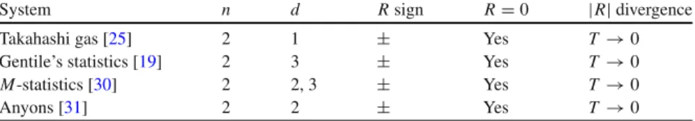
Table10.2 shows four additional models, each having R with both signs. The Takahashi gas has negative R for the gas-like phase, where attractive interactions dominate, and small|R|in the liquid-like phase. Increasing the density at constant low temperature yields a pseudophase transition from a gas-like phase to a liquid-like phase. This pseudophase transition is accompanied by a sharp positive spike in R. Conceptually simpler than the Takahashi gas are the remaining three models in Table 10.2, which are all quantum gasses intermediate between Fermions and Bosons, and
1The calculation of R for the ideal Bose gas was done with a continuous density of states, and so
Table 10.2 The thermodynamic curvature R for models where R has both signs
System n d R sign R=0 |R|divergence
Takahashi gas [25] 2 1 ± Yes T →0
Gentile’s statistics [19] 2 3 ± Yes T →0
M-statistics [30] 2 2, 3 ± Yes T →0
Anyons [31] 2 2 ± Yes T →0
In each case, R changes sign through R=0
with sign of R switching from positive to negative through R =0 on transitioning from Fermionic to Bosonic behavior. Gentile statistics have an integer parameter p giving the maximum occupation number of a state, with p=1 corresponding to a pure Fermi gas, and p→ ∞to a pure Bose gas. In the same spirit is the M-statistics model, with state occupation number M. For any temperature and chemical potential, R eventually transitions in sign from positive to negative as M increases from 1. R thus offers a convincing method of determining when the M-statistics model transitions from Fermionic to Bosonic. The quantum gas of anyons is intrinsically two-dimensional, and has particles with fractional spinαwhose variation allows us to change it continuously from a Bose gas to a Fermi gas (α:0→1); the sign of R changes correspondingly from negative to positive.
10.2.2 R for Fluid and Solid Systems, Lennard-Jones Potential
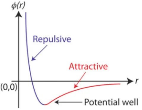
A major element in the study of fluid and solid systems is the Lennard-Jones type potential between particles, shown schematically in Fig.10.3. This potential approx-imates the interaction between particles in real fluids and solids. The Lennard-Jones type potential is strongly repulsive at short range and weakly attractive at long range. There is a minimum in the potential where repulsion and attraction balance, and where particles in a condensed liquid or solid phase like to reside. Fluid phases typically posses average separation distances between particles greater than that correspond-ing to the bottom of the potential well, and so the attractive part of the potential usually dominates. Hence, R should be mostly negative for real pure fluids, which is indeed the case. The study of the Lennard-Jones type interaction supplements that for the simple models above, and takes us a long way towards completing the picture for R for fluid and solid systems.
Fig. 10.3 The Lennard-Jones
type potential, in which two particles separated by a distance r experience a potentialφ(r), repulsive at short range and attractive at long range
T along curves with the specifiedv. Particle configurations corresponding to each situation are also shown alongside the schematic graphs.
Figure10.4a shows the ideal gas, which has R=0. Figure10.4b shows the behav-ior of R perhaps more typical of weakly interacting systems. Here, widely spaced particles interact via the attractive tail of the Lennard-Jones potential. Typically R is negative, and 0<|R| v. I characterize such situations as having “small”|R|, even in cases such as near ideal gases wherevmight get very large. The idea is that at size scales of one molecular volume, the system gets “grainy,” and thermodynamic properties such as R based on averages have increasing difficulty being accurate.
The liquid state is shown in Fig.10.4c. We have a compactly arranged, disorga-nized system of particles held together by attractive interactions, and with negative R, and|R| ∼v. On compressing the liquid state, there is the possibility of the sys-tem organizing into a crystalline solid state, where the predominant interaction is repulsive in character, with R changing sign to positive, and|R| ∼v, as shown in Fig.10.4d. Typical is a discontinuous jump from the liquid into the solid state [35]. An essential case is the critical point regime, with R shown in Fig.10.4e. There are two curves for R, separated by the critical temperature Tc. The curve at lower
temperature represents R along the coexistence curve for both liquid and vapor phases, and the curve at higher temperature represents R along the critical isochore v =vc, wherevcis the critical molar volume. R diverges to negative infinity at the
critical point along both curves. On the right side of Fig.10.4e, I sketch a near critical point particle configuration where a loose cluster has been formed by the attractive long-range tail of the Lennard-Jones type potential. The size of this cluster is given by the correlation lengthξ, with|R| ∼ ξ3. Another critical point theme is shown
in Fig.10.4f, where we have equal values of R for the coexisting liquid and vapor phases, Rl =Rv, as the two phases have identical organized droplet sizes [32–34].
Fig. 10.4 Schematic graphs for R and corresponding particle configurations: a the ideal gas, with R=0; b the weakly interacting gas, with negative R and 0<|R| v, wherevis the molecular volume; c the liquid, with negative R and|R| ∼v; d the transition from liquid to solid, with R changing sign to positive in the solid, typically discontinuously; e the critical point, with R→ −∞ and|R| ∼ ξ3; f the coexisting gas and liquid phases, with R equal in the vapor and the liquid phases very near the critical point, Rl=Rv; g an organized compact repulsive cluster held up by
Fig. 10.5 R for Water in
the coexisting liquid and vapor phases from the triple point to the critical point. Demonstrated are the points made in Fig.10.4b–g
Figure 10.4h shows the ideal Bose gas, with R always negative, and with R diverging to negative infinity as T → 0. Figure10.4i shows the ideal Fermi gas, with R always positive, and with R diverging to positive infinity as T → 0. The ideal Fermi gas shows the same qualitative behavior in 3D [18, 19] or 2D [29]. Figure10.4j shows the gas of anyons with 0 <α< 1. As we cool at constantv, starting from a high T , R starts with the Bosonic negative sign, but eventually there is a transition to the Fermionic positive sign. Aside from its intrinsic interest, the natural spatial dimension, two, of the anyon gas matches the dimension of black hole event horizons.
Lest the reader think that this is all theoretical, I show R for Water in Fig.10.5, along the coexistence curve in both the liquid and vapor phases. Figure 10.5was worked out with data from the NIST Chemistry WebBook [37,38]. R is in units of cubic nanometers, and is shown from the critical point T = Tcto the triple point
T = Tt, where Tt is the triple point temperature. Demonstrated are a number of
the principles sketched in Fig.10.4. The predominant sign of R is negative, as the attractive tail of the Lennard-Jones type potential dominates in the fluid.
In conclusion, for fluid and solid systems major elements of the thermodynamic curvature seem to be understood in principle, at least for cases with n=2 independent thermodynamic parameters. Cases with n >2, such as fluid mixtures, are largely unexplored.
10.2.3 R for Discrete Systems
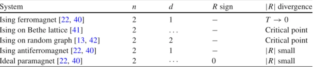
Table 10.3 The thermodynamic curvature R for several simple spin models for which R has only
one sign
System n d R sign |R|divergence
Ising ferromagnet [22,40] 2 1 − T →0 Ising on Bethe lattice [41] 2 . . . − Critical point Ising on random graph [13,42] 2 2 − Critical point Ising antiferromagnet [22,40] 2 1 − |R|small Ideal paramagnet [22,40] 2 · · · 0 |R|small
the fluid systems, then, we might think of ferromagnetic interactions as somehow “attractive.” We might also logically think of antiferromagnetic interactions, which tend to disalign adjacent spins, as “repulsive,” and with positive R. But there is little evidence that it works out like this. Mirza and Talaei [39] worked out R for a model with frustrated spins, and found a regime with large positive R. Perhaps the presence or absence of frustration is the key to interpreting the sign of R for spin systems. More calculations in spin systems would appear indicated before any definitive judgement could be made.
For spin systems, we commonly have a temperature T and a magnetic field H (more than one magnetic field may be present, but this possibility is not explored here). For such models, the partition function gets worked out in terms of β = 1/T and h = −H/T ; namely, Z = Z(β,h). The partition function leads to the thermodynamic potential per spinφ(β,h)=ln Z, and the metric elementsgαβ =
φ,αβ, in coordinatesx1,x2=(β,h)[9]. Here, we set kB=1. It is fashionable in
magnetic models to write R as
R=
φ,11 φ,12 φ,22
φ,111φ,112φ,122
φ,112φ,122φ,222
2φφ,11 φ,12 ,12 φ,22
2
. (10.9)
Many of the results for discrete models were worked out with this formula. Table10.3lists R for some spin models simple enough that R has only one sign (or R=0). The first three models in Table10.3have ferromagnetic nearest neighbor interactions. For these, R is negative, with a divergence R → −∞either as T →0 (for d=1), or at a critical point with T >0 (for d=1), as interspin coupling brings about a long-range ordering of aligned spins. This situation would appear analogous to the fluid critical point regime. The Ising antiferromagnet has a negative R with magnitude of the order of a lattice spacing, and is similar in this sense to the liquid state of the previous section.
Table 10.4 The thermodynamic curvature R for discrete models for which R has both signs
System n d R sign R=0 |R|divergence
Potts model(d>2)[13,43] 2 1 ± Yes T →0 Finite Ising ferromagnet [44] 2 1 ± Yes T →0 Ising-Heisenberg [45] 2 1 ± Yes T →0 Kagome Ising lattice [39] 2 2 ± No Critical line
per spin q. For q >2, and nonzero magnetic field, there are significant regimes of positive R at low temperature. An abrupt change in the sign of R is present in the one-dimensional Ising ferromagnet of finite N spins. R is appropriately negative for large N , but sharply increases to large positive values as N is decreased through a volume N∗ ∼ |R(N → ∞)|. Work calculating R is in progress for the one-dimensional Ising-Heisenberg model, which shows ferromagnetism, antiferromagnetism, ferri-magnetism, and frustration. The ferrimagnetic phases show substantial regimes of positive R. R for the kagome Ising lattice has recently been worked out, mostly in zero magnetic field. This model has a critical line T =Tc(H)in(T,H)space along
which R diverges on both sides, negative on the high T side with dominant ferro-magnetic interactions, and positive on the low T side with dominant ferriferro-magnetic interactions.
The physical interpretation of R for discrete systems is less conclusive than that for the fluid and solid systems. More worked examples are clearly necessary.
10.3 R for Black Hole Thermodynamics
This section discusses black hole thermodynamics, mostly in the context of general relativity [46]. String theory and other quantum black holes are beyond the scope of this talk.
10.3.1 Introduction
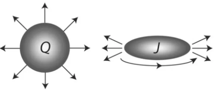
Fig. 10.6 Extremal black holes have so much charge Q that they are on the verge of exploding
out under their electrostatic repulsion, or so much angular momentum J that they are on the verge of spinning apart. Both of these scenarios, or any combination of them, are forbidden by cosmic censorship
Frequently discussed is the idea of extremal black holes. Could we add enough charge to a black hole so that it explodes outward under its electrostatic repulsion, as in Fig.10.6? Or could we add enough angular momentum so that it tears apart under its spin? Cosmic censorship forbids both these scenarios, or any combination of them. We refer to black holes as extremal if they are as close as possible to these mechanical limits. For the Kerr-Newman black hole, the condition of mechanical stability is
M4−J2−M2Q2>0. (10.10)
At the extremal limit, the black hole temperature T =0, and cosmic censorship is a way of expressing the unattainability of absolute zero temperature. It is important to appreciate, however, that the third law of thermodynamics will not always hold for black holes, as extremal black holes do not always have zero area. Hence, the black hole entropy does not always go to zero at zero temperature. This marks an important difference between black hole thermodynamics and ordinary thermodynamics.
Fig. 10.7 Fluctuating event
horizon. Are particles associ-ated with these fluctuations?
Table 10.5 Comparison
between pure fluid thermodynamics and Kerr-Newman black hole thermodynamics
Pure fluid Kerr-Newman Conserved variables (U,N,V) (M,J,Q)
Conjugate variables (T,μ,−p) (T, , )
Entropy? Yes Yes
Thermodynamic laws (0,1,2)? Yes Yes
Third law (3)? Yes No
Extensive? Yes No
Thermodynamically stable? Yes No Statistical mechanics? Yes Unclear
10.3.2 Kerr-Newman Black Hole Thermodynamics
Consider now the Kerr-Newman black hole thermodynamics, beginning with a com-parison to pure fluids; see Table10.5. First, I identify the conserved variables; these play a special role in thermodynamic fluctuation theory [49]. For Kerr-Newman black hole thermodynamics, the conserved variables are(M,J,Q), with corresponding conjugate quantities temperature T , angular velocity, and electric potential[50]. Like pure fluid thermodynamics, black hole thermodynamics has well established notions of entropy, and zeroth, first, and second laws(0,1,2)of thermodynamics. The third law(3)of thermodynamics, however, is not obeyed in Kerr-Newman black hole thermodynamics since the entropy does not go to zero at zero temperature.
this point poses few difficulties for the black hole thermodynamic fluctuation theory employed here.
Significant is the frequent absence of black hole thermodynamic stability. One manifestation of this are negative heat capacities, which are a fixture of gravita-tional thermodynamic problems. A black hole lacking thermodynamic stability can-not reach thermodynamic equilibrium with its environment, a significant deficit for the physical interpretation of any quantity, such as R, coming from thermodynamic fluctuation theory. The Kerr-Newman black hole thermodynamics is not stable for any set of values of (M,J,Q) [52]. However, stable black hole cases do exist. These result on either restricting the number of fluctuating variables, adding an AdS background, or altering the assumptions about the black hole’s topology. Stable ther-modynamic cases get most of the attention in this talk.
There is no consensus on the question of the correct microstructure support-ing black hole thermodynamics. Strsupport-ing theorists have attempted to calculate such microstructures, particularly for near extremal black holes, starting with Strominger and Vafa [53]; see Bellucci and Tiwari [54,55] and Wei et al. [56] for recent refer-ences.2In string theory calculations, the microscopic model is always explicit. By contrast, for general relativity solutions there is no evident microscopic foundation, and I direct my efforts to these in this talk.
10.3.3 Laws of Black Hole Thermodynamics
The Bekenstein-Hawking area law [57,58] sets the black hole entropy SB H
propor-tional to the area A of the event horizon:
SB H
kB =
1 4
A L2 p
, (10.11)
where
Lp=
G
c3 (10.12)
is the Planck length. Here,is Planck’s constant divided by 2π, G is the universal gravitation constant, and c is the speed of light. The area A may be calculated in terms of the conserved variables, given a black hole solution from general relativity. Such a calculation yields the full black hole thermodynamics. For example, here is the formula for A for the Kerr-Newman black hole [59]:
2If a paper starts with a spacetime metric, and calculates the thermodynamic from the area of
A=4π
2M2−Q2+2M4−J2−M2Q2. (10.13)
The black hole entropy may be added to the ordinary entropy So to get the total
entropy of the universe:
Suniver se=SB H+So. (10.14)
We generalize the second law of thermodynamics in the obvious way, that in any process starting from some initial state and going to some final state:
ΔSuniver se≥0. (10.15)
Drop now the subscript “BH” (SB H → S), and turn to the first law of black hole
thermodynamics. Writing M =M(S,J,Q)leads to
d M=T d S+d J+d Q, (10.16)
where we define the temperature
T = ∂
M
∂S
J,Q
, (10.17)
the angular velocity
=
∂ M
∂J
S,Q
, (10.18)
and the electric potential
=
∂ M
∂Q
S,J
. (10.19)
The first law of black hole thermodynamics (10.16) expresses the change in black hole energy d M to mechanical work terms,d J andd Q, and a heat term T d S.
Also essential is the 0’th law of black hole thermodynamics, which equates T to the effective surface tension of the event horizon. Calculations show this quantity to be constant over the event horizon, resulting in a unique value for the black hole temperature T .andare similarly constant over the event horizon [59].
not naturally say how this property translates to black hole thermodynamics. This point will be discussed further below in connection with black hole phase transitions.
10.3.4 Black Hole Thermodynamic Curvature R
Black hole thermodynamics leads naturally to corresponding rules for black hole ther-modynamic fluctuations, described by an information metric [49,60–62] of the type in (10.2). In conserved independent coordinates(x1,x2,x3, . . .)=(X1,X2,X3, . . .)
=(M,J,Q,· · ·), the thermodynamic metric for black hole fluctuations is (in appro-priate units)
gαβ= − ∂ 2S
∂Xα∂Xβ, (10.20)
where S is the black hole entropy. The form of the thermodynamic metric in (10.20) requires us to know S=S(X1,X2,X3, . . .). Frequently, however, we know instead M = M(Y1,Y2,Y3, . . .), where(Y1,Y2,Y3, . . .) =(S,J,Q, . . .). In this event, simplification results on writing the thermodynamic metric in the Weinhold energy form, with an additional prefactor 1/T [9,63]:
gαβ= 1
T
∂2M
∂Yα∂Yβ. (10.21)
No matter how the thermodynamic metric is written, however, we will get the same value for R for a given thermodynamic state, since R is a thermodynamic invariant.3 Thermodynamic fluctuation metrics must be positive definite for thermodynamic stability. With two independent fluctuating variables, this requires three conditions:
g11 >0, (10.22)
g22 >0, (10.23)
and
g11g22−g122 >0. (10.24)
3The line element (10.2) transforms as a scalar, since probability is a scalar quantity. Hence, the
Fig. 10.8 The event horizon
broken up into Planck area
pixels. The dark pixels are
portrayed as correlated. I propose that|R|measures the average number of correlated
pixels
Pioneering papers introducing thermodynamic curvature R into the black hole arena are [60, 65, 66]. In particular, Åman and Pidokrajt [60] first evaluated R for sev-eral solutions from gensev-eral relativity. For nondiagonal thermodynamic metrics with n =2, such as those in (10.20) and (10.21):
R= −√1
g
∂
∂x1
g
12
g11√g
∂g11
∂x2 −
1
√g∂g∂ 22
x1
+ ∂∂
x2
2
√g∂g∂ 12
x1 −
1
√g∂g∂ 11
x2 −
g12
g11√g
∂g11
∂x1
, (10.25)
where
g=g11g22−g212. (10.26)
But what is the physical interpretation of the black hole thermodynamic curvature R? In my view there is only one rational way to approach this question, and that is to follow the ideas developed in ordinary thermodynamics. It has been argued [29] that the natural units of the thermodynamic curvature are the square of the Planck length L2p. Figure10.8shows the event horizon broken up into Planck area pixels. Perhaps
|R|measures the correlation between fluctuating Planck length pixels? Since I bring no microscopic theory of black holes into play in this talk, I have no direct evidence for such a conjecture. But, by analogy with the case in ordinary thermodynamics, how else could we interpret the black hole thermodynamic curvature?
Table 10.6 The thermodynamic curvature R for black hole solutions from general relativity
Name of solution Dimension Variables Stable R sign R=0 |R|divergence Reissner-Nordström[60] 3+1 (M,Q) None 0 – None Kerr [60] 3+1 (M,J) None + No Extremal Kerr-Newman [29,60,69] 3+1 (M,J,Q) None + No Extremal Black hole [70] 4+1 (M,J) None + No Extremal Small black ring [70] 4+1 (M,J) None ± Yes Ext + crit line The solutions shown here have no regimes of thermodynamic stability. “Extremal” denotes a curve in the space of variables with T =0, and “crit” denotes a critical line with T =0, along which|R|
diverges
10.3.5 Solutions from General Relativity
The thermodynamic curvature R for black holes has been worked out for a number of systems, and I make no attempt to be complete in my reporting below. Rather, I present some thoughts about how results from various general relativity solutions might be compared with one another, and to solutions from ordinary thermodynamics. In Tables10.6and10.7, I consider only thermodynamic states with S>0, M >0, and T > 0. Within this physical range of variables, the solutions divide into two categories, those for which there are no regimes satisfying thermodynamic stability (10.22)–(10.24), and those for which there are such regimes. In either category, R can be readily worked out from (10.25); it is real in all the cases I calculated. However, the physical interpretation I have presented for R for ordinary thermodynamics is based on fluctuation theory, and this assumes thermodynamic stability. I key on the stable cases below.
Table 10.6 shows results for R for several general relativity solutions having no stable thermodynamic states. Tabulated are the dimension (spatial+time), the fluctuating conserved variables, whether or not there are regimes of thermodynamic stability (no cases in Table10.6), the sign of R (or an indication “0” if R is identically zero), whether or not there are places where the sign of R changes through zero, and whether or not there are divergences |R| → ∞. Of the older solutions: Reissner-Nordström, Kerr, and Kerr-Newman, none are thermodynamically stable for any thermodynamic state. Also, not thermodynamically stable are the two solutions listed with a higher dimension=4+1. Some of the older solutions have been worked out in higher dimensions, but with no reports of thermodynamically stable cases [68].
Table10.7shows results for R for several general relativity solutions with “some” or “all” states thermodynamically stable. Thermodynamic stability results on either adding an AdS background, restricting the number of fluctuating variables, or altering the assumptions about the black hole’s topology.
Table 10.7 The thermodynamic curvature R for black hole solutions from general relativity
Name of solution Dimension Variables Stable R sign R=0 |R|divergence BTZ [60,66] 2+1 (M,J) All 0 0 None RN-AdS [60,71–73] 3+1 (M,Q) Some ± Yes Ext + crit line K-AdS [72,74,75] 3+1 (M,J) Some − No Critical line Restricted KN [29,49] 3+1 (J,Q) All + No Extremal Large black ring [70] 4+1 (M,J) All − No Ext + crit line These solutions all have at least some thermodynamically stable regimes. The characterization of
R is based only on states in the stable regime. “Extremal” denotes a curve in the space of variables
with T =0, and “crit” denote a critical line with T =0 along which|R|diverges
is shown schematically in Fig.10.9a, and it resembles the behavior for the ideal gas in Fig.10.4a.
In the thermodynamically stable regime, Reissner-Nordström-AdS black holes have an extremal curve T =0, as well as a line of critical points where|R|diverges to infinity. This critical line obtains for Q<Qc, where the critical value Qcdepends
on the cosmological constant. For a fixed Q>Qc, as we reduce T from a large value,
R diverges to positive infinity at the extremal curve. However, for fixed Q<Qc, as
we reduce T from a large value, R diverges to negative infinity along the critical line. As T is decreased further, we enter a thermodynamically unstable regime followed by a stable regime where R increases.
The general black hole thermodynamic behavior for RN-AdS has been associated with a phase transition analogous to a van der Waals model by Chamblin et al. [76,77]. A number of researchers have calculated R for this case [60,71–73]. The behavior of R for RN-AdS is shown schematically in Fig.10.9b. For Q > Qc the
behavior of R resembles that in the Fermi gas, shown in Fig.10.4i. For Q<Qc, R
resembles the critical point behavior in Fig.10.4e. This correspondence is certainly consistent with the association with the van der Waals model. I add that the Q<Qc
curve in Fig.10.9b has a bump resembling the one in Fig.10.4g.
Kerr-AdS black holes have no extremal curve in the thermodynamically stable regime. However, a critical line depending on the cosmological constant bounds the thermodynamically stable regime at low T . Along this critical line, R diverges to negative infinity. For the Kerr-AdS black hole thermodynamics, R is always negative. Figure10.9c sketches R as T is decreased from a large value at constant J . The sketch resembles the critical point behavior in Fig.10.4e. However, once we cross the critical line, there are no more thermodynamically stable regimes. Banerjee et al. [78,79] have discussed phase transitions in AdS black holes using the Ehrenfest relations, with special attention to the orders of the phase transitions.
Fig. 10.9 Schematic graphs for R for thermodynamically stable general relativistic black hole
solutions: a the BTZ solution, with R =0; b the RN-AdS solution, with R diverging to positive infinity at the extremal curve for Q>Qc, and with R diverging to negative infinity, at temperature
Tc >0, along the critical line for Q <Qc; c the K-AdS solution, with R diverging to negative
infinity at the critical line, d the restricted KN(J,Q)solution, with R diverging to positive infinity at the extremal limit; e the large black ring solution, with R diverging to positive infinity at the
extremal curve, and with R diverging to negative infinity along the critical line
The large black ring solution also has significant regimes of stability, bounded by an extremal curve and a critical line. R diverges to positive infinity at the extremal curve, and to negative infinity along the critical line.
A few patterns present themselves for the thermodynamically stable general rel-ativity solutions considered in this section. In all cases, the divergence of R at the extremal curve is to positive infinity, resembling in this sense the divergence for the ideal Fermi gasses from ordinary thermodynamics. Where there are critical lines (with|R|diverging with T =0), the divergence of R is to negative infinity, resem-bling the critical point divergences in ordinary thermodynamics. But I have consid-ered too few cases here to assert with any confidence that these patterns are general. Further study is obviously necessary.
10.3.6 Discussion of “Inconsistencies”
Much debated in black hole thermodynamics has been the possibility raised by Davies [50] that the curve of diverging heat capacity CJ,Q = T(∂S/∂T)J,Q in
the Kerr-Newman black hole solution corresponds to a phase transition. Diverging heat capacities are a feature of second-order phase transitions in ordinary fluid and spin systems, so Davies’ association would appear logical.
Closer examination, however, raises some questions about Davies’ correspon-dence. First, an ordinary thermodynamic system generally has at its foundation some known microscopic model. Such a model offers direct insight not only into the char-acter of the thermodynamic variables, but into the microscopic signatures of any thermodynamic anomaly. In the absence of a known microscopic model we have dif-ficulty answering basic questions. If some heat capacity diverges, how could we be sure that we have not just made an inappropriate choice of thermodynamic variables, which reveals infinities with no really fundamental significance? What do we make of curves in thermodynamic state space where one heat capacity diverges, but the other heat capacities stay regular? What if various heat capacities diverge along different curves, as happens in the Kerr-Newman black hole [29,52], as in Fig.10.10. Which curve corresponds to a true phase transition? One of them? All of them? Perhaps it is safer to associate curves of diverging R with black hole phase transitions. R has a unique status in identifying microscopic order from thermodynamics. and ordering at the microscopic level is at the foundation of phase transitions.
Fig. 10.10 Characteristic
curves for the Kerr-Newman black hole. The curve along which CJ,Qdiverges is the
Davies curve. R diverges
at the extremal limit and along curves corresponding to a change of thermodynamic stability, which have diverging
CJ,and C,Q. R does not
diverge along the Davies
curve. Hereα=J2/M4and β=Q2/M2
a nonstatistical force holding the assembly together, and a result R =0, where the unknown constituents move independently of each other, would make perfect sense.
10.4 Conclusions
What are black holes made out of? This question has not been answered here. How-ever, one way to address this question is by following an agenda of matching the statistical mechanics of known microscopic models to black hole thermodynamic solutions from general relativity, or other theories of gravity. I hope that I have con-vinced the audience that the thermodynamic curvature R has a contribution to make to this game.
I have given a broad survey of thermodynamic curvature R, one spanning results in fluids and solids, spin systems, and black hole thermodynamics. R results from the unique thermodynamic information metric giving thermodynamic fluctuations. R has a unique status in thermodynamics as being a geometric invariant, the same for any given thermodynamic state no matter what coordinates we calculate in. In ordinary thermodynamics, the sign of R indicates the character of microscopic interactions, and|R|indicates the average size of organized fluctuations. Although I have given no direct evidence that this interpretation holds for black hole thermodynamics, if we believe in the broad generality of thermodynamic principles, this interpretation of R should transcend specific scenarios.
Acknowledgments I thank George Skestos for travel support, and I thank the conference organizer
Stefano Bellucci of INFN for giving me the opportunity to present my work.
References
1. F. Weinhold, Thermodynamics and geometry. Phys. Today 29(3), 23 (1976)
2. G. Ruppeiner, Thermodynamics: a Riemannian geometric model. Phys. Rev. A 20, 1608 (1979) 3. B. Andresen, P. Salamon, R.S. Berry, Thermodynamics in finite time. Phys. Today 37(9), 62
(1984)
4. G. Ruppeiner, Thermodynamic curvature: pure fluids to black holes. J. Phys.: Conf. Series 410, 012138 (2013)
5. L. Landau, E. Lifshitz, Statistical Physics (Pergamon, New York, 1977) 6. R.K. Pathria, Statistical Mechanics (Butterworth-Heinemann, Oxford, 1996)
7. A. Einstein, On the general molecular theory of heat. Ann. Phys. (Leipzig) 14, 354 (1904) 8. A. Einstein, The theory of the opalescence of homogeneous fluids and liquid mixtures near the
critical state. Ann. Phys. (Leipzig) 33, 1275 (1910)
9. G. Ruppeiner, Riemannian geometry in thermodynamic fluctuation theory. Rev. Mod. Phys.
67, 605 (1995)
10. G. Ruppeiner, Riemannian geometry in thermodynamic fluctuation theory. Rev. Mod. Phys.
68, 313(E) (1996)
11. D. Laugwitz, Differential and Riemannian Geometry (Academic, New York, 1965)
12. G. Ruppeiner, Thermodynamic curvature measures interactions. Am. J. Phys. 78, 1170 (2010) 13. D.A. Johnston, W. Janke, R. Kenna, Information geometry, one, two, three (and four). Acta
Phys. Pol. B 34, 4923 (2003)
14. G. Ruppeiner, New thermodynamic fluctuation theory using path integrals. Phys. Rev. A 27, 1116 (1983)
15. G. Ruppeiner, Thermodynamic critical fluctuation theory? Phys. Rev. Lett. 50, 287 (1983) 16. L. Diósi, B. Lukács, Covariant evolution equation for the thermodynamic fluctuations. Phys.
Rev. A 31, 3415 (1985)
17. S. Weinberg, Gravitation and Cosmology (Wiley, New York, 1972)
18. H. Janyszek, R. Mrugała, Riemannian geometry and stability of ideal quantum gases. J. Phys. A: Math. Gen. 23, 467 (1990)
19. H. Oshima, T. Obata, H. Hara, Riemann scalar curvature of ideal quantum gases obeying Gentile’s statistics. J. Phys. A 32, 6373 (1999)
20. B. Mirza, H. Mohammadzadeh, Thermodynamic geometry of deformed bosons and fermions. J. Phys. A: Math. Gen. 44, 475003 (2011)
21. D. Brody, N. Rivier, Geometrical aspects of statistical mechanics. Phys. Rev. E 51, 1006 (1995) 22. H. Janyszek, R. Mrugała, Riemannian geometry and the thermodynamics of model magnetic
systems. Phys. Rev. A 39, 6515 (1989)
23. D.C. Brody, D.W. Hook, Information geometry in vapour–liquid equilibrium. J. Phys. A: Math. Theor. 42, 023001 (2009)
24. W. Janke, D.A. Johnston, R. Kenna, Information geometry of the spherical model. Phys. Rev. E 67, 046106 (2003)
25. G. Ruppeiner, J. Chance, Thermodynamic curvature of a one-dimensional fluid. J. Chem. Phys.
92, 3700 (1990)
26. J. Nulton, P. Salamon, Geometry of the ideal gas. Phys. Rev. A 31, 2520 (1985)
27. G. Ruppeiner, C. Davis, Thermodynamic curvature of the multicomponent ideal gas. Phys. Rev. A 41, 2200 (1990)
29. G. Ruppeiner, Thermodynamic curvature and phase transitions in Kerr-Newman black holes. Phys. Rev. D 78, 024016 (2008)
30. M.R. Ubriaco, Stability and anyonic behavior of systems with M-statistics. Physica A 392, 4868 (2013).arXiv:1302.4719[hep-th]
31. B. Mirza, H. Mohammadzadeh, Nonperturbative thermodynamic geometry of anyon gas. Phys. Rev. E 80, 011132 (2009)
32. G. Ruppeiner, Thermodynamic curvature from the critical point to the triple point. Phys. Rev. E 86, 021130 (2012)
33. G. Ruppeiner, A. Sahay, T. Sarkar, G. Sengupta, Thermodynamic geometry, phase transitions, and the Widom line. Phys. Rev. E 86, 052103 (2012).arXiv:1106.2270[hep-th]
34. H.-O. May, P. Mausbach, Riemannian geometry study of vapor–liquid phase equilibria and supercritical behavior of the Lennard–Jones fluid. Phys. Rev. E 85, 031201 (2012)
35. H.-O. May, P. Mausbach, G. Ruppeiner, Thermodynamic curvature for attractive and repulsive intermolecular forces. Phys. Rev. E. 88, 032123 (2013)
36. E. Johansson, K. Bolton, P. Ahlström, Simulations of vapor water clusters at vapor–liquid equilibrium. J. Chem. Phys. 123, 024504 (2005)
37. NIST Chemistry WebBook, available at the Web Sitehttp://webbook.nist.gov/chemistry/
38. W. Wagner, A. Pruss, The IAPWS formulation 1995 for the thermodynamic properties of ordinary water substance for general and scientific use. J. Phys. Chem. Ref. Data 31, 387 (2002)
39. B. Mirza, Z. Talaei, Thermodynamic geometry of a kagome Ising model in a magnetic field. Phys. Lett. A 377, 513 (2013)
40. G. Ruppeiner, Application of Riemannian geometry to the thermodynamics of a simple fluc-tuating magnetic system. Phys. Rev. A 24, 488 (1981)
41. B.P. Dolan, Geometry and thermodynamic fluctuations of the Ising model on a Bethe lattice. Proc. R. Soc. London A 454, 2655 (1998)
42. W. Janke, D.A. Johnston, R.P.K.C. Malmini, Information geometry of the Ising model on planar random graphs. Phys. Rev. E 66, 056119 (2002)
43. B.P. Dolan, D.A. Johnston, R. Kenna, The information geometry of the one-dimensional Potts model. J. Phys. A: Math. Gen. 35, 9025 (2002)
44. D.C. Brody, A. Ritz, Information geometry of finite Ising models. J. Geom. Phys. 47, 207 (2003)
45. To be submitted.
46. J.D. Bekenstein, Black-hole thermodynamics. Phys. Today 33(1), 24 (1980)
47. C.W. Misner, K.S. Thorne, J.A. Wheeler, Gravitation (Freeman, San Francisco, 1973) 48. G.N. Lewis, Generalized thermodynamics including the theory of fluctuations. J. Am. Chem.
Soc. 53, 2578 (1931)
49. G. Ruppeiner, Stability and fluctuations in black hole thermodynamics. Phys. Rev. D 75, 024037 (2007)
50. P. Davies, The thermodynamic theory of black holes. Proc. R. Soc. London A 353, 499 (1977) 51. P.T. Landsberg, D. Tranah, Thermodynamics of non-extensive entropies. Collect. Phenom. 3,
73 (1980)
52. D. Tranah, P.T. Landsberg, Thermodynamics of non-extensive entropies. Collect. Phenom. 3, 81 (1980)
53. A. Strominger, C. Vafa, Microscopic origin of the Bekenstein–Hawking entropy. Phys. Lett. B
379, 99 (1996)
54. S. Bellucci, B.N. Tiwari, State-space correlations and stabilities. Phys. Rev. D 82, 084008 (2010)
55. S. Bellucci, B.N. Tiwari, Thermodynamic geometry and topological Einstein-Yang-Mills black holes. Entropy 14, 1045 (2012)
56. S.-W. Wei, Y.-X. Liu, Critical phenomena and thermodynamic geometry of charged Gauss– Bonnet AdS black holes. Phys. Rev. D 87, 044014 (2013)
58. S. Hawking, Black holes and thermodynamics. Phys. Rev. D 13, 191 (1976) 59. L. Smarr, Mass formula for Kerr black holes. Phys. Rev. Lett. 30, 71 (1973)
60. J. Åman, I. Bengtsson, N. Pidokrajt, Geometry of black hole thermodynamics. Gen. Relativ. Gravit. 35, 1733 (2003)
61. D. Pavón, J.M. Rubí, Thermodynamical fluctuations of a massive Schwarzschild black hole. Phys. Lett. 99A, 214 (1983)
62. D. Pavón, J.M. Rubí, Kerr black hole thermodynamical fluctuations. Gen. Relativ. Gravit. 17, 387 (1985)
63. P. Salamon, J.D. Nulton, E. Ihrig, On the relation between entropy and energy versions of thermodynamic length. J. Chem. Phys. 80, 436 (1984)
64. H. Quevedo, Geometrothermodynamics of black holes. Gen. Relativ. Gravit. 40, 971 (2008) 65. S. Ferrara, G. Gibbons, R. Kallosh, Black holes and critical points in moduli space. Nuc. Phys.
B 500, 75 (1997)
66. R.G. Cai, J.H. Cho, Thermodynamic curvature of the BTZ black hole. Phys. Rev. D 60, 067502 (1999)
67. K.S. Thorne, R.H. Price, D.A. Macdonald, Black Holes: The Membrane Paradigm (Yale Uni-versity Press, New Haven, 1986)
68. J.E. Åman, N. Pidokrajt, Geometry of higher-dimensional black hole thermodynamics. Phys. Rev. D 73, 024017 (2006)
69. B. Mirza, M. Zamaninasab, Ruppeiner geometry of RN black holes: flat or curved? JHEP 1006, 059 (2007)
70. G. Arcioni, E. Lozano-Tellechea, Stability and critical phenomena of black holes and black rings. Phys. Rev. D 72, 104021 (2005)
71. J. Shen, R.-G. Cai, B. Wang, R.-K. Su, Thermodynamic geometry and critical behavior of black holes. Int. J. Mod. Phys. A 22, 11 (2007)
72. A. Sahay, T. Sarkar, G. Sengupta, On the thermodynamic geometry and critical phenomena of AdS black holes. JHEP 1007, 82 (2010)
73. C. Niu, Y. Tian, X.-N. Wu, Critical phenomena and thermodynamic geometry of Reissner-Nordström-anti-de Sitter black holes. Phys. Rev. D 85, 024017 (2012)
74. R. Banerjee, S.K. Modak, S. Samanta, Second order phase transition and thermodynamic geometry in Kerr-AdS black holes. Phys. Rev. D 84, 064024 (2011)
75. Y.-D. Tsai, X.-N. Wu, Y. Yang, Phase structure of the Kerr-AdS black hole. Phys. Rev. D 85, 044005 (2012)
76. A. Chamblin, R. Emparan, C.V. Johnson, R.C. Myers, Charged AdS black holes and catastrophic holography. Phys. Rev. D 60, 064018 (1999)
77. A. Chamblin, R. Emparan, C.V. Johnson, R.C. Myers, Holography, thermodynamics, and fluc-tuations of charged AdS black holes. Phys. Rev. D 60, 104026 (1999)
78. R. Banerjee, S. Ghosh, D. Roychowdhury: New type of phase transition in Reissner-Nordstrom-¨ AdS black hole and its thermodynamic geometry. Phys. Lett. B 696, 156 (2011)
79. R. Banerjee, S. Modak, D. Roychowdhury, A unified picture of phase transition: from liquid– vapour systems to AdS black holes. JHEP 1210, 125 (2012)