Selection works both ways: BMI and marital formation
among young women
Michael Malcolm•Ilker Kaya
Received: 16 September 2013 / Accepted: 17 April 2014
ÓSpringer Science+Business Media New York 2014
Abstract The literature on entry into marriages has almost universally regarded a high body mass index (BMI) to be a disadvantage for women in the marriage market. But the theoretical effect of BMI on marital entry is actually uncertain because women who anticipate poor outcomes in the marriage market are more likely to accept early offers, while women with more desirable characteristics can afford to wait for a better match. Using data from the 1997 National Longitudinal Survey of Youth, we show that female entry into marriage does decline as BMI rises, but that early marriage is nonlinear in BMI. Women with an extremely high BMI or with a BMI in the most attractive range are less likely to marry early.
Keywords BMIObesityMarital formation
JEL Classification I10J12
1 Introduction
Marital status and obesity have undergone substantial and coincident changes. About 69 % of American adults were overweight or obese as of 2010, a figure which has increased by more than 50 % in the last 30 years.1 Marriage rates are 39 % lower than they were in 1950, with 17 % of this drop occurring since 2000.
M. Malcolm (&)
Department of Economics, West Chester University of Pennsylvania, West Chester, PA, USA e-mail: [email protected]
I. Kaya
Department of Economics, American University of Sharjah, Sharjah, United Arab Emirates e-mail: [email protected]
Marriages that do form are delayed; the proportion of women between 25 and 34 who have never been married is more than 150 % higher than it was in 1970. This paper explores one aspect of the relationship between marital status and obesity.
The relationship between body mass index (BMI) and marital status is complex, and features bidirectional causality. A low BMI is a desirable characteristic in the marriage market, but at the same time being married can alter the incentives for investment in one’s health. Our paper focuses on the first point—the relationship between BMI and entry into marriage, specifically for women.
Being obese is generally regarded to be a negative attribute in the marriage market, especially for women. For example, Averett et al. (2008) find that the negative association between BMI and marital entry is significant for both genders, but is much stronger for women than it is for men. Analyses of Internet dating websites find that a low body weight is a desirable characteristic for women (e.g. Hitsch et al.2010).2
But even if we take for granted that a low BMI makes women more desirable in the marriage market, the translation between desirability and entry into marriages is not immediate. If we think of selection as a two-way process, the effect of desirability on marital entry is theoretically ambiguous. While it may be the case that obese women have more difficulty locating high-quality partners, they consequently have more incentive to commit to a relationship with matches that do arrive. That is, women with less desirable physical characteristics may actually be more likely to enter into marriages quickly because of bad expectations about future prospects. By contrast, women who perceive themselves to be the most desirable might delay getting married because they hope to locate a better match. Overall, the selection effect of BMI into marital entry is ambiguous.
Our paper uses data from the 1997 cohort of the National Longitudinal Survey of Youth (NLSY97) to investigate this relationship. In contrast to earlier work, we find mixed results on the effect of BMI on marital entry. Overall, marital probability does decline as BMI rises, but early marriages are different. We find evidence that women with a BMI in the most attractive range are lesslikely to enter into early marriages, as are women with a very high BMI. Similarly, extrapolating over the whole life cycle, increases in BMI are associated with a later age at first marriage. But, for women who marry early, increases in BMI are associated with alowerage at first marriage. Earlier work, by combining women in different age groups into a single sample to develop parameter estimates, has not detected this effect. By better understanding how our characteristics and our behavioral choices impact incentives and outcomes related to family structure, we can make some progress in understanding changes in family dynamics.
The paper proceeds as follows. Section2 briefly reviews the literature on the relationship between BMI and marriage. Section3presents a theoretical model of the relationship between marital formation and characteristics like BMI that index desirability. Section4 discusses the data and results. Section5concludes.
2
2 Related literature
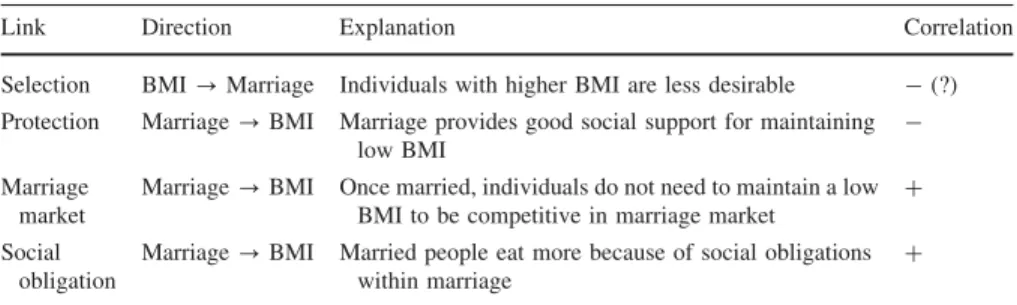
Averett et al. (2008) describe four causal links between marriage and BMI. The table below summarizes these links, and gives the implied correlation between marriage and BMI (Table1).
With respect to the three hypotheses that posit a causal link from marriage to BMI, the consensus appears to be that the overall effect is positive. Averett et al. (2008) find that marriage results in an increase in BMI for both partners and that BMI falls again following divorces. This finding is supported by Averett et al. (2013), who find a positive impact on BMI both for marital and cohabiting relationships.3
The main focus of this paper relates to selection. With respect to link, it does appear unequivocal that a high BMI is an undesirable characteristic for women in terms of their ability to locate partners. Cawley et al. (2006) find that overweight teenage girls have difficulty dating, and Ali et al. (2014) find that overweight white teenage girls are less likely to have engaged in sexual activity of any kind. Hitsch et al. (2010) find that overweight women find fewer matches on dating websites.4 Importantly, these papers analyze only the ability to locate a match, and there is a clear negative selection effect. Marriage is not the same thing observationally, because it involves not only locating a match, but choosing to form a commitment. The effect of deteriorated attractiveness on the marriage market appears to be that women with a higher BMI have more difficulty locating husbands and, when they do, they marry husbands with less desirable characteristics. Oreffice and Quintana-Domeque (2010) show significant assortative matching between husbands and wives. Specifically, they find that BMI is the most important anthropometric covariate for women, and that heavier women tend to marry husbands who are shorter, and with lower income and education levels. Chiappori et al. (2012) explicitly calculate the tradeoff between BMI and various other attributes in the marriage market. Offer (2001) argues that the importance of low BMI for women on the marriage market has grown in recent decades because of the declining value of female household production. Lin et al. (2012) find that black women under-invest in maintaining a healthy BMI because of the incarceration rate of black men and consequent poor expectations about the marriage market.5Mukhopadhyay (2008) finds a negative selection effect for both marriage and cohabitation.
In summary, it appears that the BMI?marriage link rationalizes a negative empirical correlation between BMI and marital status, while the marriage?BMI link rationalizes a positive correlation in the data. This presents an econometric difficulty. One-shot analysis of the relationship between contemporaneous marital status and BMI is difficult to parse because of the concatenated causal effects, and
3
There are improvements in some health outcomes, including mental health and alcohol abuse.
4
There are also negative consequences in the employment market. Hammermesh and Biddle (1994) is the seminal paper. This effect, of course, can spill over into the marriage market because it affects potential gains from marriage.
5
there are various strategies for dealing with this issue. Averett et al. (2008) regress BMI on marital status and contrast outcomes with and without individual fixed effects in order to purge selection bias. Mukhopadhyay (2008) lags obesity by one period before the marriage to capture the selection effect. Averett and Korenman (1996) use a seven-year lag.
Despite the extensive literature on this point, earlier authors seem not to have recognized that a negative sign for the selection effect into marriage is not necessarily obvious. Recent literature on marital formation treats the problem as a sequence of offers, which can be accepted or rejected. To put it succinctly, selection works both ways—women differ in terms of the offers that they receive, but they also choose whom and when to marry among offers that are forthcoming. Women with a high BMI may have fewer and lower-quality opportunities to marry, but they have more incentive to select into offers that do arrive. We proceed now to a theoretical analysis that explores this possibility, followed by an empirical analysis shows this non-monotonic effect, especially among marriages that occur before age 25.
3 Theory
We present a simple model showing that a higher desirability parameter does not necessarily translate into a higher marriage rate in any given period. Suppose that a woman lives through an infinite sequence of periods in which she faces probability
pof locating a partner each period, wherepis our proxy for desirability. The quality of arriving partners is indexed byx, wherexhas distributionf(x) and is independent and identically distributed across arrivals.6 We assume that this distribution has positive support over the interval [xL,xH].
When a woman receives a match of qualityxshe has two choices. First, she can enter into a marriage, which generates lifetime utilityh(x): the net present value of a marital union for a woman, including the risk of divorce.h(x) is a weakly increasing function of partner quality x. Under standard Nash bargaining models, a higher-Table 1 Theoretical links between marriage and BMI
Link Direction Explanation Correlation
Selection BMI?Marriage Individuals with higher BMI are less desirable -(?) Protection Marriage?BMI Marriage provides good social support for maintaining
low BMI
-Marriage market
Marriage?BMI Once married, individuals do not need to maintain a low BMI to be competitive in marriage market
?
Social obligation
Marriage?BMI Married people eat more because of social obligations within marriage
?
6
quality husband can lead to higher marital surplus, but the fraction of that surplus that accrues to the wife is dependent upon the bargaining shares. In the extreme case, female marital utility could be constant in partner quality,h(x)=h, if the man claims all of the surplus brought to the marriage from his partner quality. Otherwise, when the surplus is split,h(x) is increasing inx.
The second option is that the woman can reject the match and remain single. The current-period utility from remaining single is normalized to 0. In subsequent periods, single women receive a new match each period with probability p, with
xdrawn independently for each match.
Given the structure of the problem, the equilibrium is a reservation-type equilibrium where matches are accepted when their value exceeds some thresholdx. LettingE designate the expected value of a draw from the match distributionf(x), we can use the stationarity of the problem to calculate it as such:
E¼r x
xL
0þd pEþX 1
i¼1
dið1pÞipE
!
" #
fðxÞdxþr xH
xh x
ð Þ fðxÞdx
¼rx
xL dp
1dð1pÞEfðxÞdxþr xH
x
hð Þ x fðxÞdx
ð1Þ
In words, when the draw ofxfalls in the interval½xL;x, the match is rejected and the current utility is 0. In future periods, a match arrives with probabilityp, leading to a reiteration of the same problem. It is possible in this model to have a succession of one or more periods with no match before the next match arrives. Future payoffs are discounted at rated. When the draw of partner quality xfalls in the interval
x; xH
½ , the match is accepted, leading to utilityh(x).
Where new draws lead to an expected valueE, the woman enters into a marriage with her current partner whenever her utility in marriage is higher than her expected utility of remaining single. Again, by remaining single, the woman in future periods receives a draw with probabilityp, but also faces a chance of repeated periods with no forthcoming match.
hð Þ x 0þd pEþX 1
i¼1
dið1pÞipE
!
ð2Þ
Assuming forward-rational expectations, we can combine (1) and (2) to calculate the reservation partner qualityx. For the extreme case wherehð Þ ¼x his constant, thenx¼0. If all matches generate the same (positive) utility, then the first match will always be accepted. However, whenh(x) is increasing inx, then the reservation quality levelxis increasing inp. The expected value of a new match is increasing in
probability of accepting offers therefore falls as p rises. Among offers that are forthcoming, women with good rematch prospects reject more offers.
To link this to observable data, the empirically observed probability that a woman with rematch probability p will accept offers for marriage in any given period is pPrðxxÞ. This emphasizes the two-step nature of the process. To observe a marriage in the data, there must be both an offer and an acceptance. This observable marriage rate pPrðxxÞ can be either increasing or decreasing in p
since PrðxxÞis decreasing inp. The most desirable women get more offers, but they also reject more offers. Thus, it is possible in the data to observe an increase or a decrease in the number of marriages resulting from the selection effect of a BMI in the most desirable range.
The implicit assumption that higher desirability leads necessarily to more marriage can be generated as the special case of this model where h(x)=h is constant. In this case, all matches are accepted and so the marriage rate in any given period is justp. But once we allow for increasing husband quality to raise the wife’s utility, it is important to take account of both steps of the process—offer and then acceptance.
While our model focuses on forward-rational choices from one side of the market, this result can easily be interpreted in the context of two-way matching models. For example, in the Gale-Shapley stable marriage problem (Gale and Shapley1962), the solution algorithm involves men sequentially proffering offers to their most preferred single woman, but female acceptance of these offers is only conditional. For the most desirable women, a match (characterized as an engagement) may dissolve if the woman receives a proposal from a more desirable man later on. So although the most desirable women may enjoy better initial offers, they also have more opportunities to subsequently dissolve their relationships with their initial partners.
To relate this to earlier literature, Averett et al. (2008) assert that ‘‘obesity does not necessarily prevent marriage but it may influence marital timing and mate quality.’’ This statement is correct, but the influence on marital timing is not obvious. Either direction is possible, since there are contrary effects pulling in opposite directions.
4 Data and results
The sample uses all available data in the NLSY97 from 1997 to 2010. There are 4,385 women in the sample, all of whom were between age 13 and age 17 at the first observation in 1997. The actual sample size is reduced because of missing data issues for some variables.7
A steadily rising proportion of women in the sample married as they aged. Figure1shows the proportion of women who are married at various ages, both for
7
all women in the sample and for women with 12 or fewer years of education. Early marriage rates are higher for women with 12 or fewer years of education, converging as age rises.
BMI is calculated usingBMI¼weightðin KGÞ heightðin MÞ
½ 2. A BMI below 18.5 is considered to
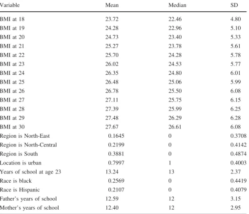
be underweight. A BMI between 18.5 and 25 is in the healthy range, while BMI’s between 25 and 30, and those above 30, are classified as in the overweight and obese range, respectively. Calculated BMI’s below 10 or above 45 are dropped from the sample, as these presumably are the consequence of misreported height and weight data.8 Table2 gives descriptive statistics on BMI by age. Mean BMI rose from 23.72 to 27.67 as the women in our sample aged from 18 to 30. The distributions are right-skewed, with the mean exceeding the median. Correlations between a woman’s BMI at ages between 18 and 29 are high. Even over intervals as long as 10 years, these correlations are all greater than 0.7.9
We will first use nonparametric techniques to contrast women at various ages who choose to marry with those who choose to remain single. These are difficult to interpret causally, but they present a clear picture of the data. We then proceed to reduced-form structural models to develop estimates of the magnitude and statistical significance of these relationships.
To begin exploring the selection effect of BMI into marital entry, we consider the pool of women who are single at ageXand contrast the BMI characteristics at age
Xbetween those women who are married at ageX?2 and those women who are still single at ageX?2.
There are a two methodological notes. First, the time interval between the age
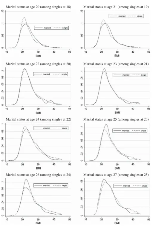
X BMI observation and the ageX?2 marital observation is not a full two years because the BMI observation is taken at the end of the year, but the marital observation at age X?2 is taken in August. So, in reality the gap is around 18 months, which is a typical engagement period.10 The idea is that some people will be forming commitments but report themselves as single at ageXand then will have married by ageX ?2. Second, at each age, a few of the single women were pregnant at the ageXBMI observation, so these were dropped from the sample.11 Figure2 presents kernel density estimates that illustrate what we describe above.12Among the population of women who are single at ageX, we estimate the density of BMI’s from ageXamong those women who are married at ageX?2 and those women who are still single at ageX?2. This allows us to contrast the BMI characteristics of these two groups. Among women who are single at ageX, who is more likely to be married at age X?2?
8
In various years, between 6 and 118 observations were dropped for a BMI out of range: less than 3 % of the sample in any given year.
9
The full results are available upon request from the author.
10 Average Engagement Length, and Other Wedding Planning Statistics (2013). 11
Fewer than 5 % of females from our sample, in any year, were unmarried and pregnant. We do not drop women who were pregnant at ageX?2, since the analysis focuses on the effect of BMI at ageXon entry into marriages in succeeding periods.
12
Fig. 1 Proportion married by age
Table 2 Descriptive statistics
Variable Mean Median SD
BMI at 18 23.72 22.46 4.80
BMI at 19 24.28 22.96 5.10
BMI at 20 24.73 23.40 5.33
BMI at 21 25.27 23.78 5.61
BMI at 22 25.70 24.28 5.78
BMI at 23 26.02 24.53 5.77
BMI at 24 26.35 24.80 6.01
BMI at 25 26.48 25.06 5.99
BMI at 26 26.78 25.50 6.08
BMI at 27 27.11 25.75 6.15
BMI at 28 27.39 25.99 6.25
BMI at 29 27.48 26.29 6.28
BMI at 30 27.67 26.61 6.08
Region is North-East 0.1645 0 0.3708
Region is North-Central 0.2199 0 0.4142
Region is South 0.3881 0 0.4874
Location is urban 0.7997 1 0.4003
Years of school at age 23 13.24 13 2.37
Race is black 0.2569 0 0.4419
Race is Hispanic 0.2107 0 0.4079
Father’s years of school 12.59 12 3.15
Mother’s years of school 12.40 12 2.95
Marital status at age 20 (among singles at 18) Marital status at age 21 (among singles at 19)
Marital status at age 22 (among singles at 20) Marital status at age 23 (among singles at 21)
Marital status at age 24 (among singles at 22) Marital status at age 25 (among singles at 23)
Marital status at age 26 (among singles at 24) Marital status at age 27 (among singles at 25)
For early marriages, those occurring between ages 18–20 and between ages 19–21, there is a distinctly nonlinear pattern. In these age groups, marriage is actually most likely among women who start out as moderately overweight. Those with a BMI in the most desirable range and those with a BMI in the obese range are more likely to be single. These choices can be easily rationalized in terms of our theoretical model—women with a high BMI have trouble locating partners, but women with a low BMI do not marry early because they will face no trouble locating matches later on and can afford to continue searching. For women entering into first marriages at the ages of 22, 23 and 24, we can see a slight nonlinearity of the variety mentioned above, although the distributions are close. However, by age 25, there is a clear negative selection effect of BMI into marriage.
To be clear, this is a descriptive analysis rather than a causal analysis. While the temporal structure purges reverse-causation problems, there could be unobserved covariates with BMI that are also correlated with marital choices. Nevertheless, there are two important points to take away. First, the relationship between BMI and future marital status is notprima facienegative, either theoretically or empirically. Second, there is a potential that the underlying structural parameters vary by age. In other words, low BMI may have a positive selection effect into marriage for women in some age groups and a negative effect for women in other age groups.
The most serious barrier to a causal interpretation of these results is that individual socioeconomic conditions are correlated with BMI, and of course socioeconomic conditions also affect choices related to marital entry.13We proceed by developing reduced form parametric models that control for these socioeconomic variations.
Averett et al. (2008) control for education levels, race, region and whether the respondent lives in an urban or a rural area. Regional variations and the urban/rural divide create differences in marriage market opportunities. Education levels and race are standard controls in the literature. We begin with these controls, and for some regressions we also add educational attainment of the respondent’s mother and father as a more direct control for the family’s socioeconomic status. However, measurements of the parents’ education levels are not available for all respondents and including these variables reduces the sample size by almost 25 %. Thus, throughout we report results both with and without these regressors. Table2 contains descriptive statistics for these control variables.
First, in line with what other authors have done, we consider a regression for whether a woman ever married at any point over the panel; the oldest women in the 2010 wave of this dataset are 30. We consider this as a function of the woman’s BMI at age 20 and also add the demographic controls discussed above, also measured at age 20. This is similar to the approach followed by Averett and Korenman (1996), who use a seven-year lag.14However, we measured education at age 23 in order to capture variations in human capital and job market potential.
13
The literature on the correlation between BMI and socioeconomic status is extensive. Baum and Ruhm (2009) investigate important intermediating factors.
14
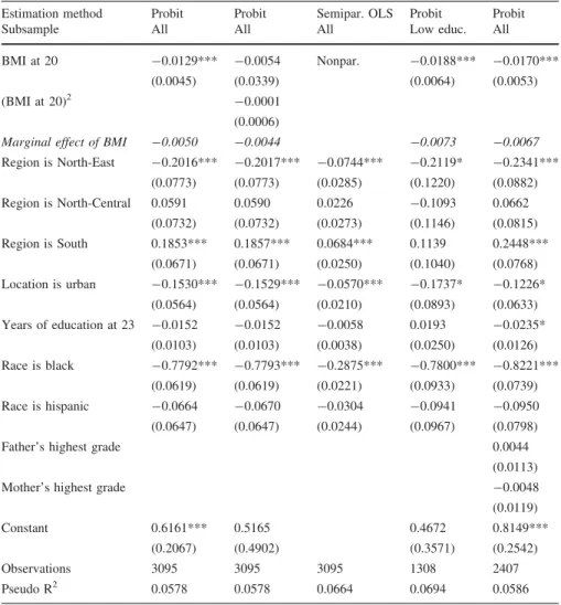
Table3 presents the results, along with calculated marginal effects of a BMI increase, evaluated at the mean. In line with what other authors have found, the association between marital entry and BMI is negative and the coefficient is significant at the 1 % level. In the probit specification using the entire sample, each unit increase in BMI is associated with a 0.5 % decline in the probability of marriage. For the subsample of women with 12 or fewer years of education, the marginal effect is 0.73 %.
In these specifications, BMI enters the model linearly, which may be overly restrictive. To address potential nonlinearities, we first consider a parametric Table 3 Was woman ever married over panel?
Estimation method Probit Probit Semipar. OLS Probit Probit
Subsample All All All Low educ. All
BMI at 20 -0.0129*** (0.0045)
-0.0054 (0.0339)
Nonpar. -0.0188*** (0.0064)
-0.0170*** (0.0053) (BMI at 20)2 -0.0001
(0.0006)
Marginal effect of BMI -0.0050 -0.0044 -0.0073 -0.0067
Region is North-East -0.2016*** (0.0773) -0.2017*** (0.0773) -0.0744*** (0.0285) -0.2119* (0.1220) -0.2341*** (0.0882) Region is North-Central 0.0591
(0.0732) 0.0590 (0.0732) 0.0226 (0.0273) -0.1093 (0.1146) 0.0662 (0.0815) Region is South 0.1853***
(0.0671) 0.1857*** (0.0671) 0.0684*** (0.0250) 0.1139 (0.1040) 0.2448*** (0.0768) Location is urban -0.1530***
(0.0564) -0.1529*** (0.0564) -0.0570*** (0.0210) -0.1737* (0.0893) -0.1226* (0.0633) Years of education at 23 -0.0152
(0.0103) -0.0152 (0.0103) -0.0058 (0.0038) 0.0193 (0.0250) -0.0235* (0.0126) Race is black -0.7792***
(0.0619) -0.7793*** (0.0619) -0.2875*** (0.0221) -0.7800*** (0.0933) -0.8221*** (0.0739) Race is hispanic -0.0664
(0.0647) -0.0670 (0.0647) -0.0304 (0.0244) -0.0941 (0.0967) -0.0950 (0.0798)
Father’s highest grade 0.0044
(0.0113)
Mother’s highest grade -0.0048
(0.0119) Constant 0.6161*** (0.2067) 0.5165 (0.4902) 0.4672 (0.3571) 0.8149*** (0.2542)
Observations 3095 3095 3095 1308 2407
Pseudo R2 0.0578 0.0578 0.0664 0.0694 0.0586 Italicized row is not independent variables, but calculated marginal effects
specification with a quadratic term in BMI, which fails to produce any significant relationship. Finally, to allow for as much generality as possible, we consider a semiparametric OLS model in which the control variables enter linearly but where BMI enters nonparametrically.15 The semiparametric estimate of the relationship between BMI and marriage probability is shown in Fig.3. There is a downward slope overall, but it is mostly active for BMI’s higher than about 25. For BMI’s in the healthy range, changes in BMI have little impact on marital probability. Above a BMI of about 25, increases in BMI are strongly associated with lower marital probability. This nonlinearity is consistent with a penalty specifically associated with obesity rather than with BMI increases over all ranges. The results in Conley and Glauber (2007), for example, suggest an ‘‘obesity penalty.’’
The signs of the other coefficients are as expected. Girls from the Northeast and who live in urban areas are less likely to marry (or at least they delay their marriages past the age observed in this sample), as are blacks. Increases in education are associated with declines in marital probability, although the coefficient is not significant at conventional levels.
While the results presented in Table3appear to be a standard negative selection result, the descriptive results cited earlier suggest that the story might be different for early marriages. Thus, we repeat the same exercise as above, but instead of considering whether a woman was ever married over the panel, we study whether the woman was married at age 25.16
These results are presented in Table4. Using a linear term in BMI appears to show no significant effect of BMI on early marital entry, but this is only a numerical artifact that results from a strongly nonlinear effect. When we include a quadratic expansion for BMI, the higher-order term is significant at the 5 % level. The signs Fig. 3 Semiparametric estimate—was woman ever married?
15
Robinson (1988) first proposed this estimator and outlined its properties. We again use a Gaussian kernel for the nonparametric component, with bandwidth chosen to minimize mean square error.
16
of the coefficients imply that the probability of early marriage initiallyrisesas BMI rises, and then begins to fall. Direct calculation using the model with the full sample shows that maximum marriage probability for these early marriages occurs at
BMI=25.3, slightly overweight, and falls in either direction. The same relationship is clear from the semiparametric estimate, which is shown in Fig.4. Marriage probability falls as BMI rises higher than aroundBMI=25 (the obesity penalty), but it also falls as BMI dropslowerthan this critical value. This can be rationalized in terms of the model presented earlier. Women with a BMI that is too high have difficulty locating partners, but women with a BMI in the most desirable range do Table 4 Was woman married at age 25?
Estimation method Probit Probit Semipar. OLS Probit Probit
Subsample All All All Low educ. All
BMI at 20 -0.0065 (0.0048)
0.0685* (0.0364)
Nonpar. -0.0115* (0.0067)
0.1105** (0.0438) (BMI at 20)2 -0.0014**
(0.0007)
-0.0022*** (0.0008)
Marginal effect of BMI -0.0023 0.0007 -0.0041 0.0011
Region is North-East -0.3896*** (0.0832) -0.3915*** (0.0833) -0.1227*** (0.0271) -0.4689*** (0.1289) -0.4102*** (0.0956) Region is North-Central 0.0199
(0.0760) 0.0186 (0.0760) 0.0080 (0.0261) -0.1718 (0.1176) 0.0549 (0.0847) Region is South 0.1222*
(0.0694) 0.1251* (0.0694) 0.0428* (0.0239) -0.0049 (0.1059) 0.1876** (0.0795) Location is urban -0.1588***
(0.0585) -0.1590*** (0.0585) -0.0558*** (0.0200) -0.1445 (0.0917) -0.1512** (0.0659) Years of education at 23 -0.0477***
(0.0108) -0.0475*** (0.0108) -0.0166*** (0.0037) 0.0366 (0.0262) -0.0562*** (0.0132) Race is black -0.7443***
(0.0665) -0.7461*** (0.0665) -0.2402*** (0.0211) -0.8677*** (0.0993) -0.7917*** (0.0800) Race is hispanic -0.0786
(0.0670) -0.0835 (0.0670) -0.0338 (0.0233) -0.1655* (0.0986) -0.1001 (0.0831)
Father’s highest grade -0.0024
(0.0118)
Mother’s highest grade 0.0007
(0.0125) Constant 0.6476*** (0.2157) -0.3428 (0.5221) -0.0259 (0.3745) -0.7225 (0.6264)
Observations 3027 3027 3027 1289 2354
Pseudo R2 0.0578 0.0589 0.0635 0.0808 0.0638 Italicized row is not independent variables, but calculated marginal effects
Dependent variable equal to 1 if woman was ever married by age 25. Geographical variables are those measured at age 20. West is the dropped region and white/other is the dropped racial category. Standard errors are given in parentheses. Marginal effects are evaluated at the mean
not marry early because they can afford to wait for higher-quality matches later. Note that the effect of education onearlymarital entry is negative and significant. When we restrict our estimation to the subsample of women with no college education, the quadratic term is no longer significant, and in fact the marginal effect of BMI is negative even for early marriages; the coefficient is significant at the 10 % level. It is worth noting that, both for early marriages and for marriages across the entire panel, the negative impact of BMI on marital probability is stronger for women with low education than it is across the entire sample. This may be evidence for a result along the lines of Chiappori et al. (2012) that various marriageability attributes can trade off for each other. BMI appears to be a more important factor for women who are less competitive on human capital dimensions.
We have presented the previous specifications to contrast them with closely-related specifications that appear elsewhere in the literature, and have shown that the results may crucially depend upon the age group chosen. Another empirical strategy is to attack the question by studying the determinants of age at first marriage. OLS is inappropriate for this estimation because many women, about 56 %, have never married over the sample period. Over 90 % of Americans eventually marry, and so true age at marriage is a latent variable in our dataset. If we letyindicate a woman’s true age at first marriage, we observeyas long asy\y*, but only observe that the woman is not yet married by agey* wheny[y*. Here,y* is the oldest age at which women in our dataset our observed, which is age 30.
With this in mind, we use a tobit model to study how age at marriage is impacted by BMI, and other control variables, where we regard age at marriage to be a latent variable that is censored above at age 30. In order to capture the selection effect, we again need to consider BMI before marriage as the determinant. Our strategy is to fix BMI at age 20 and determine how this impacts age at marriage. This specification implicitly exploits the fact that intertemporal correlation in BMI for an individual is high, so that BMI at age 20 is informative about the pre-marriage desirability characteristics for a woman who marries at a later age.
Table5 presents the results of this tobit regression. Across specifications, a higher BMI is associated with a higher age at first marriage. This result is significant at the 10 % level for the estimation over the full sample, but is significant at the 5 % level for the subsample of no-college women. We again note that the marginal effect is substantially stronger for low-educated women. Each unit increase in BMI is associated with a 0.12-year increase in age at first marriage for women with no college versus a 0.07-year increase for all women.
Table 5 Determinants of age at first marriage
Estimation method Tobit Tobit Tobit Tobit
Subsample All All Low educ. All
BMI at 20 0.0675*
(0.0367) -0.2333 (0.2719) 0.1184** (0.0562) 0.0945** (0.0411)
(BMI at 20)2 0.0055
(0.0049)
Marginal effect of BMI 0.0675 0.0358 0.1184 0.0945
Region is North-East 2.1436*** (0.6270) 2.1543*** (0.6268) 3.3020*** (1.0953) 2.7111*** (0.6881) Region is North-Central -0.7097
(0.5756) -0.7099 (0.5753) 1.0680 (0.9898) -0.5303 (0.6145) Region is South -2.0806***
(0.5216) -2.0845*** (0.5214) -1.6473* (0.8692) -2.1664*** (0.5733) Location is urban 1.1539**
(0.4704) 1.1498** (0.4702) 1.1218 (0.8050) 0.9133* (0.5080) Years of education at 23 0.4373***
(0.0810) 0.4386*** (0.0810) 0.1704 (0.2155) 0.4253*** (0.0954) Race is black 7.2317***
(0.5198) 7.2298*** (0.5196) 8.4546*** (0.8616) 7.4354*** (0.6009) Race is hispanic -0.3972
(0.5029) -0.3724 (0.5031) -0.1664 (0.8009) 0.2222 (0.6077)
Father’s highest grade 0.0899
(0.0852)
Mother’s highest grade 0.0208
(0.0898) Constant 22.96*** (1.63) 26.89*** (3.87) 24.12*** (3.10) 20.91*** (1.93)
Observations 3058 3058 1287 2377
Pseudo R2 0.0264 0.0265 0.0321 0.0270
Number of censored observations (age[30) 1,732 1,732 722 1,326 Italicized row is not independent variables, but calculated marginal effects
Dependent variable equal to age at first marriage, which truncated for the NLSY97 above age 30. Geographical variables are those measured at age 20. Women who were pregnant at age 20 are dropped from the sample. West is the dropped region and white/other is the dropped racial category. Standard errors are given in parentheses. Marginal effects are evaluated at the mean
When examining over a woman’s entire life cycle, a higher BMI creates a barrier to marriage, as other researchers find, but the story may be different for early marriages. Figure5 shows an analogous semiparametric regression of age at first marriage, but specifically for women who married at some point over the sample (before age 30). In this case, we see that estimated age at first marriagedeclinesas BMI rises, until BMI reaches approximately 28, at which point age at first marriage begins rising with increases in BMI.
In line with the previous result, we estimate a parametric model of age at first marriage specifically for women who married at some point over the panel. This is less than half of all women in the sample. The specifications above use BMI at a fixed age, and then exploit intertemporal correlation in BMI’s across age groups. A different empirical strategy is to analyze age at first marriage as a function of the woman’s BMI two years prior to the marriage.17Of course, this estimation is only possible for women who married over the sample period. We rescale BMI as a percentile relative to other women at that age. In other words, ‘‘BMI two years before marriage’’ could be BMI at age 19 for one woman and BMI at age 28 for another woman. But these two cannot be measured against the same scale because the entire BMI distribution shifts as women age. Thus, BMI measurements and all other continuous variables for this analysis are normalized to percentiles relative to all women in that age demographic.
The results of these OLS regressions are given in Table6. Women with a higher rank in the percentile BMI distribution prior to marriage are, on average, those women who marry at ayoungerage. The result is significant at the 1 % level for the full sample, and is consistent with the semiparametric estimate in Fig.5. Again we see that the selection effect of high BMI into delayed marital entry is not obvious. At least among women who marry before the age of 30, it appears that those with a higher BMI are actually more likely to marry at ayoungerage.
Fig. 5 Semiparametric estimate—age at first marriage for women married over observation period
17
To summarize the results, the kernel density estimates in Fig.2 show that the relationship between BMI and entry into marriage may be nonmonotonic, especially for early marriages. In line with what other authors have found, Table3and Fig.3 show that the probability of entry into marriage before the age of 30 is negatively impacted by BMI, especially for BMI’s in the obese range. But when we restrict ourselves to marriages before the age of 25, as given in Table4 and Fig.4, the relationship is nonmonotonic. Early marriages are less likely among women with high BMIandamong women with a BMI in the most desirable range; the maximum Table 6 Determinants of age at first marriage among married women
Estimation method OLS OLS OLS OLS
Subsample All All Low educ. All
% BMI two years before marriage -0.8183*** (0.2666) -0.0812 (1.0417) -0.4997 (0.3636) -0.6458** (0.2905) (% BMI two years before marriage)2 -0.7534
(1.0293)
Marginal effect of % BMI -0.8183 -0.8037 -0.4997 -0.6458
Region is North-East 0.9215*** (0.2580) 0.9280*** (0.2582) 0.7354** (0.3665) 0.8335*** (0.2847) Region is North-Central -0.1550
(0.2255) -0.1589 (0.2256) -0.5944* (0.3166) -0.2423 (0.2401) Region is South -0.1306
(0.2030) -0.1325 (0.2030) -0.3284 (0.2827) -0.1609 (0.2211) Location is urban 0.9450***
(0.1796) 0.9408*** (0.1798) 0.2986 (0.2504) 0.9730*** (0.1944) % Highest grade two years before marriage 1.4803***
(0.2622) 1.4670*** (0.2629) -2.4536*** (0.4319) 1.1443*** (0.3039) Race is black 0.5726***
(0.2223) 0.5723*** (0.2224) 1.6196*** (0.3110) 0.6633** (0.2563) Race is hispanic -0.8766***
(0.1917) -0.8794*** (0.1918) -0.5471** (0.2569) -0.2105 (0.2347)
Father’s highest grade 0.1045***
(0.0338)
Mother’s highest grade 0.0918**
(0.0361) Constant 21.8733*** (0.3034) 21.7643*** (0.3380) 22.9730*** (0.4088) 19.4921 (0.5066)
Observations 1396 1396 667 1112
R2 0.0911 0.0914 0.1205 0.1278
Italicized row is not independent variables, but calculated marginal effects
Dependent variable equal to age at first marriage. All variables are those measured two years before marriage. BMI and education level are rescaled as percentiles relative to all observed women at that age. West is the dropped region and white/other is the dropped racial category. Standard errors are given in parentheses
point is slightly above the upper limit for a healthy BMI. When we study age at first marriage extrapolated over a woman’s entire life cycle, Table5 shows that age at first marriage increases in BMI. But if we restrict our sample to those women who married during the sample period, Table6and Fig.5show that, for these women, age at first marriage actually declines as BMI rises, at least up to some critical point well into the overweight range.
5 Conclusion
Averett et al. (2008) stated that ‘‘theory suggests a clear sign for the selection effect—those who are healthy (i.e. thinner) are most likely to be selected into marriage.’’ We emphasize here that ‘‘selected into marriage’’ is not the same thing as ‘‘marry’’. Selection works both ways. Different women may face a different arrival rate and quality of partners, but they also make a choice about whether to marry potential spouses who do arrive. These two contrasting effects pull the impact of desirability on marital entry in opposite directions—higher desirability means a higher probability of finding a match, but italsomeans good future prospects and hence the ability to reject suboptimal matches with low risk.
By taking another look at longitudinal data on BMI and marital behavior, we have explored this possibility and have shown that this nonmonotonic theoretical effect is in fact represented in women’s observed choices. Early marriages are less likely among women with very high BMI’sandamong women with BMI’s in the most attractive range. Correspondingly, age at first marriage overall rises in BMI, but early marriages are different.
Helen Coster was widely lampooned for an April, 2013 article in the Daily Princetonian, where she urged young women not to wait too long before getting married to a high-quality husband, but her argument captures the essence of this decision problem. Even women with access to high-quality matches may forego early partnering as long as they expect their future prospects to be strong.
As potential spouses delay marriage, the marriage market endogenously becomes more dynamic, even at later ages. We have shown in this paper that, in their decisionmaking, women apparently take into account not only their present set of opportunities but also their future set of likely opportunities. Otherwise, it is difficult to rationalize any circumstance under which women with higher desirability characteristics are less likely to enter into marriages.
References
Averett, S., & Korenman, S. (1996). The economic reality of the beauty myth. Journal of Human Resources, 31(2), 304–330.
Averett, S. L., Sikora, A., & Argys, L. M. (2008). For better or worse: Relationship status and body mass index.Economics & Human Biology, 6(3), 330–349.
Baum, C. L, I. I., & Ruhm, C. J. (2009). Age, socioeconomic status and obesity growth.Journal of Health Economics, 28(3), 635–648.
Cawley, J., Joyner, K., & Sobal, J. (2006). Size matters the influence of adolescents’ weight and height on dating and sex.Rationality and Society, 18(1), 67–94.
Chiappori, P. A., Oreffice, S., & Quintana-Domeque, C. (2012). Fatter attraction: Anthropometric and socioeconomic matching on the marriage market.Journal of Political Economy, 120(4), 659–695. Conley, D., & Glauber, R. (2007). Gender, body mass, and socioeconomic status: New evidence from the
PSID.Advances in Health Economics and Health Services Research, 17, 253–275.
Coster, H. (2013, April 4). Advice for the young women of Princeton (and colleges everywhere).The Daily Princetonian.
Gale, D., & Shapley, L. S. (1962). College admissions and the stability of marriage.The American Mathematical Monthly, 69(1), 9–15.
Hamermesh, D. S., & Biddle, J. E. (1994). Beauty and the labor market.The American Economic Review, 84(5), 1174–1194.
Health, United States (2011). National Center for Health Statistics.
Hitsch, G. J., Hortac¸su, A., & Ariely, D. (2010). What makes you click?—Mate preferences in online dating.Quantitative Marketing and Economics, 8(4), 393–427.
Lin, W., McEvilly, K., & Pantano, J. (2012). Obesity and Marriage Markets. Working paper. Mukhopadhyay, S. (2008). Do women value marriage more? The effect of obesity on cohabitation and
marriage in the USA.Review of Economics of the Household, 6(2), 111–126.
Offer, A. (2001). Body weight and self-control in the United States and Britain since the 1950s.Social History of Medicine, 14(1), 79–106.
Oreffice, S., & Quintana-Domeque, C. (2010). Anthropometry and socioeconomics among couples: Evidence in the United States.Economics & Human Biology, 8(3), 373–384.