IMPROVING ENRICHMENT STRATEGIES IN OUTCOME-DEPENDENT SAMPLING DESIGNS AND ADAPTIVE BIOMARKER-THRESHOLD DESIGNS
Ting Wang
A dissertation submitted to the faculty at the University of North Carolina at Chapel Hill in partial fulfillment of the requirements for the degree of Doctor of Philosophy in the
Department of Biostatistics in the Gillings School of Global Public Health.
Chapel Hill 2020
c 2020 Ting Wang
ABSTRACT
Ting Wang: Improving Enrichment Strategies in Outcome-Dependent Sampling Designs and Adaptive Biomarker-Threshold Designs
(Under the direction of Haibo Zhou and Xiaofei Wang)
In many study areas, such as epidemiological studies and clinical trials, both enrichment schemes and estimation methods have been investigated to achieve more efficient estimates of interest given fixed budget. In this dissertation, we study how to improve outcome-dependent-sampling (ODS) designs in epidemiological studies and adaptive enrichment designs in the ongoing randomized clinical trials, in the ways of both enrichment strategies and estimation methods. Bayesian method plays an important role in all topics by providing robust posterior or reasonable prediction based on all the available information.
In Topic 1, we propose a new cost-effective sampling design, the extreme outcome dependent sampling (EODS) design and a Bayesian inference procedure, for studies with a continuous outcome. Compared to existing ODS designs, the new EODS design adopts a strategy to use the smallest and largest outcomes to identify supplemental samples. The EODS design provides an alternative way to make efficient use of limited resources, especially in multi-state studies, by targeting the more informative subjects for sampling. We develop a Bayesian Markov Chain Monte Carlo (MCMC) method for the EODS design. Our method can incorporate the information of all subjects, including those with unobserved exposure, and provide an unbiased and efficient estimator through posterior inference. Simulation results indicate that the newly proposed EODS scheme, coupled with the proposed MCMC estimator, is more efficient than the existing ODS designs and the simple random sampling design with the same sample size.
we propose the likelihood dependent sampling (LDS) design, for studies with a continuous outcome. Compared to existing ODS designs, the LDS design selects supplemental samples from those subjects with the smallest estimated conditional likelihood values, and thus allows those subjects to directly impact the likelihood function. The proposed LDS design provides a new way to make efficient use of the limited resources for second stage sampling. Bayesian MCMC method is also used for inference of data from LDS design. Simulation results indicate that the newly proposed sampling scheme, coupled with the proposed MCMC estimator, is more efficient than existing ODS designs and the simple random sampling design.
ACKNOWLEDGEMENTS
TABLE OF CONTENTS
LIST OF TABLES . . . x
LIST OF FIGURES . . . xi
CHAPTER 1: INTRODUCTION . . . 1
CHAPTER 2: LITERATURE REVIEW . . . 5
2.1 Outcome-Dependent Sampling Designs . . . 5
2.1.1 Case-control, Case-cohort and Outcome-Dependent Sampling Designs 5 2.1.2 Statistical Inference Methods for ODS Designs . . . 11
2.2 Motivating Designs . . . 21
2.2.1 Extreme Value Design and Examples . . . 21
2.2.2 Biomarker-Driven Clinical Trials . . . 24
2.3 Bayesian methods and Missing Data Approaches . . . 36
2.3.1 Bayesian MCMC . . . 37
2.3.2 Other Missing Data Approaches . . . 42
2.3.3 Predictive Probability of Success through Bayesian Method . . . 45
2.4 Outline of Proposed Work . . . 47
2.4.1 Bayesian Inference for Extreme-Outcome Dependent Sampling Design 47 2.4.2 Bayesian Inference for Likelihood-Dependent Sampling Design . . . . 50
2.4.3 Design and Analysis of Biomarker-Integrated Clinical Trials with Adaptive Threshold Detection and Flexible Patient Enrichment . . . 53
CHAPTER 3: BAYESIAN INFERENCE FOR EXTREME OUTCOME-DEPENDENT SAMPLING DESIGN . . . 60
3.1 Introduction . . . 60
3.3 Bayesian MCMC Inference . . . 62
3.4 Simulation Studies . . . 65
3.5 Analysis of the Collaborative Perinatal Project Data . . . 69
3.6 Concluding Remarks . . . 72
CHAPTER 4: BAYESIAN INFERENCE FOR LIKELIHOOD-DEPEND-ENT SAMPLING DESIGN . . . 74
4.1 Introduction . . . 74
4.2 Designs and Data Structure . . . 74
4.3 Bayesian MCMC Inference . . . 76
4.4 Simulation Studies . . . 78
4.5 Analysis of the Collaborative Perinatal Project Data . . . 81
4.6 Concluding Remarks . . . 83
CHAPTER 5: DESIGN AND ANALYSIS OF BIOMARKER-INTEGRA-TED CLINICAL TRIALS WITH ADAPTIVE THRESHOLD DETEC-TION AND FLEXIBLE PATIENT ENRICHMENT . . . 85
5.1 Introduction . . . 85
5.2 Design . . . 87
5.2.1 Notation and assumptions . . . 87
5.2.2 Design procedures . . . 88
5.3 Methods . . . 89
5.3.1 Estimator of biomarker threshold and its asymptotic variance . . . . 89
5.3.2 Calculation of the Predictive Probability of Success / Failure . . . 91
5.4 Estimation and Test of Treatment Effects . . . 92
5.5 Simulation Studies . . . 93
5.6 Analysis of the JAVELIN Lung 200 Data . . . 103
5.7 Concluding Remarks . . . 104
CHAPTER 6: SUMMARY AND FUTURE RESEARCH . . . 107
6.1 Summary . . . 107
LIST OF TABLES
3.1 Simulation results of the EODS design with NormalX . . . 67
3.2 Simulation results of the EODS design with a mixture distribution ofX . . . 68
3.3 Analysis results of the EODS design for the Collaborative Perinatal Project data set . . . 71
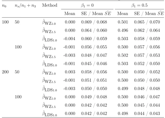
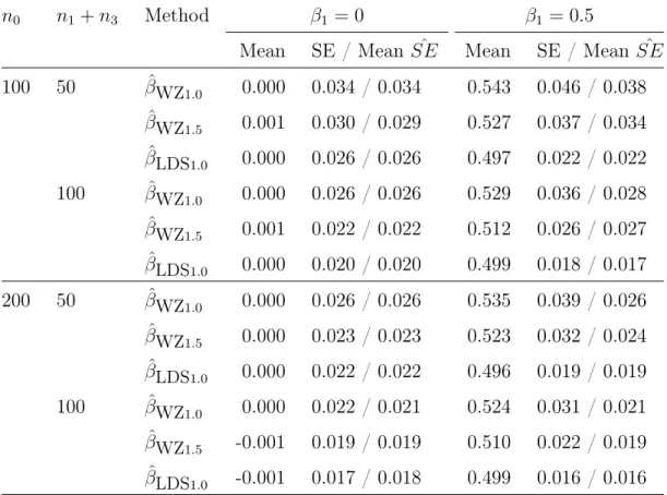
4.1 Simulation results of the LDS design with Normal X . . . 79
4.2 Simulation results of the LDS design with a mixture distribution of X . . . . 80
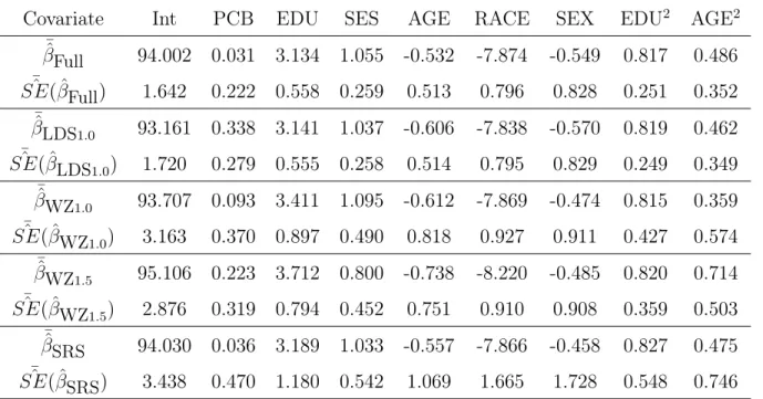
4.3 Analysis results of the LDS design for the Collaborative Perinatal Project data set . . . 82
5.1 Threshold Estimation, Futility Rate and Other Operating Characteristics . . 96
5.2 Test and Estimation of Treatment Effect in Positives . . . 98
5.3 Test and Estimation of Treatment Effect in Negatives . . . 99
5.4 Test and Estimation of Overall Treatment Effect . . . 100
5.5 Threshold Estimation, Futility Rate and Other Operating Characteristics of The Special Case . . . 101
5.6 Test and Estimation of Treatment Effects of The Special Case . . . 101
5.7 Major change of design outputs whenc0 = 0.5 and t= 0.5 . . . 102
5.8 Response Rates in Barlesi et al. (2018) . . . 103
5.9 Threshold Estimation, Futility Rate and Other Operating Characteristics of the example . . . 104
5.10 Test and Estimation of Treatment Effects of the example . . . 105
LIST OF FIGURES
2.1 Flow chart of some common Biomarker-Driven Designs. . . 28 2.2 Flow chart of some enriched Biomarker-Driven Designs. . . 31 2.3 Flow Chart of the Biomarker Enrichment and Adaptive
CHAPTER 1: INTRODUCTION
[Why ODS?] If budget permitted, investigators would like to collect all the data in a study population. However, this is usually not the case as large epidemiology studies or clinical trials typically require recruiting thousands of subjects and long time to follow up. In many epidemiological studies, the primary outcome variable is easy to obtain, while some exposure variables are expensive to measure. This motivates statisticians to develop outcome-dependent sampling (ODS) designs. In such designs, the probability of observing the exposure/covariate for a subject depends on the observed value of the outcome variable. By oversampling certain subjects, ODS design allows investigators to concentrate the resources on the segment of the population that are most informative in explaining the outcome/exposure relationship. ODS designs, coupled with appropriate analysis, provides more efficient estimates than standard statistical analysis based on a simple random sample.
[Development of ODS designs] For studies with binary outcome (i.e. the disease occurrence status), case-control design has been widely used since Cornfield (1951), Cox (1970), and Breslow and Cain (1988). When the disease is rare, much of the information collected on disease free subjects is redundant. Case-control design addresses this issue by oversampling the cases. Zhou et al. (2002) developed ODS schemes for continuous outcome, with further development by Weaver and Zhou (2005), Song et al. (2009) and Zhou et al. (2014). Ding et al. (2014) applied ODS designs to failure-time data and Pan et al. (2018) analyzed the secondary outcome for data obtained from the ODS design. We will review them in detail in the next chapter.
that when we are interested in regression of some response y on covariate x, “the selection of individuals with values ofxvarying within broad limits would give us more precision.". Royall (1970) further revived the old idea of purposive selection and showed that in many situations purposive selection, such as choosing the largest x values, will be superior to probability proportional to size selection with the appropriate regression estimators. This motivates us to consider using extreme sampling based on outcome to select the supplemental samples in the ODS designs. Moreover, stratified extreme sampling can further make estimation more robust.
[Motivation: likelihood dependent sampling] In ODS and PDS designs, we search both lower and upper tails of the distribution of the observed Y values or use the predicted chance of a subject’s unobserved X, conditional on its Y and Z, locating in (−∞, XL] or (XU,∞), as the criterion to select the supplemental samples. However, we never know whether
the lower tail or the upper tail has better candidates as the supplemental samples. Thus, a criterion providing us the order of the qualification for the supplemental sample of all samples except SRS would help us find more informative supplemental samples. This motivates us to consider the conditional likelihood, the conditional density of outcome and the covariate of interest, as a new criterion. The conditional likelihood contains the information of both Y and estimated X with small likelihood implying the rarity of the sample and thus considered as more informative. Moreover, we can use lower tail of the likelihood as the unique direction to find the better supplemental sample instead of searching both lower and upper tails of the outcome or the estimated covariate of interest.
there often exists no validated “optimal" thresholds at patient randomization. The need for a study design that builds a prospective procedure to co-investigating biomarker threshold and treatment effects in the identified patient population during the trial has motivated the development of adaptive threshold detection and patient enrichment designs (ATED) (Simon and Simon, 2013; Lai et al., 2014; Ohwada and Morita, 2016; Simon and Simon, 2017; Zhang et al., 2017; Diao et al., 2018; Xu et al., 2019). In these designs, the target population is adaptively learned, the biomarker threshold is adaptively estimated, and future patient enrollment is restricted to the patients who are identified as “positives". However, these designs have largely ignored investigation of the estimation accuracy of the biomarker threshold and the estimation of treatment effects. They also focus on testing the treatment effect in biomarker-positive patients, aggressively excluding biomarker-negative patients in early stage, thereby preventing accurate estimation of the biomarker threshold and the treatment effect in biomarker-negative patients.
CHAPTER 2: LITERATURE REVIEW
2.1 Outcome-Dependent Sampling Designs
2.1.1 Case-control, Case-cohort and Outcome-Dependent Sampling Designs
In this section, we will review case-control, case-cohort and Outcome-Dependent Sampling (ODS) designs.
Case-control and Case-cohort Designs
In epidemiological observational studies, the investigators would like to concentrate resources where there is the greatest amount of information. This motivates statisticians to develop different outcome-dependent sampling strategies according to the nature of the primary outcome. When the primary outcome is binary, case-control design (Cornfield, 1951; Cox, 1970; Breslow and Cain, 1988) is often preferred. Case-control studies are retrospective. Study subjects with the outcome of interest (case) are compared to a control group, and then researchers retrospectively retrieve the exposure and covariate information. As discussed in Breslow and Powers (1978) and Prentice and Pyke (1979), the prospective and retrospective models lead to identical maximum likelihood estimates of the odds ratios for case-control data. This means that standard logistic regression could be applied to the case-control study as if the data had been obtained in a prospective study.
other covariates are measured on these four random subsamples. When the disease and exposure is rare, four groups would have quite different sizes. The observations from the small groups will have more information than observations from the larger groups. Hence, this two stage design will be more efficient than a similar one stage design. Breslow and Cain (1988) considers the two-stage case-control study, and proposed a modified logistic regression.
In the first stage, disease status and easy to obtain covariates are obtained for a large number of subjects. Then in the second stage, expensive exposure is measured for a case-control sample from the general population. Flanders and Greenland (1991) showed how to use pseudo-likelihood approach to analyze two stage case-control data. Zhao and Lipsitz (1992) reviewed twelve two-stage designs, which include two-stage case-control and case-cohort as special case.
The case-cohort study design was originally proposed by Prentice (1986), which is also a well known outcome-dependent sampling design used to study the association between a time-to-event outcome and risk factors. In case-cohort design, the expensive exposure is only measured on a simple random sample (SRS) of the full cohort and on all the failure individuals. The main advantage of the case-cohort study design over a cohort study is that full covariate data are only needed on the cases and SRS individuals, not all the original cohort, potentially saving time and money if measures such as biomarkers or genotypes are required. And the advantage of a case-cohort study over a nested case-control study is that the same SRS can be used as the comparison group for studying different diseases, rather than identifying a new set of controls for each disease. Also, the process of obtaining measurements on baseline samples from individuals in the SRS can be initiated at any time after the original cohort has been set up, whereas in a nested case-control study the cases need to be identified before the controls can be defined and the measurement process begin.
event (Prentice, 1986),. Different weighting methods have been described in detail (Barlow et al., 1999) and compared by simulation (Onland-Moret et al., 2007). The usual standard error estimates from the Cox PH model are not valid in the weighted versions, and should be replaced by alternatives such as a robust jack-knife estimator (Barlow, 1994).
Outcome-Dependent Sampling Designs with continuous outcomes
In many studies, the primary outcome is measured on a continuous scale. Outcome-Dependent Sampling (ODS) design was proposed for the continuous outcome, which includes a simple random sample from the underlying population and some additional supplemental samples that are drawn from regions of the outcome space that are of particular interest. The advantage of such ODS designs is that, while providing overall information about the population, it allows the investigators to oversample certain segments of the population that are believed to be more informative.
However, for data obtained via complex sampling designs such as those described above, the usual methods of analysis are no longer applicable. In particular, maximum likelihood assuming i.i.d data and ordinary least squares both render estimators that are inconsistent, as was shown by Holt et al. (1980). In practice, investigators usually dichotomize the continuous outcome based on whether it is above or below a certain cut off point. However, some efficiency is lost by converting a continuous outcome into dichotomous scale (Suissa, 1991). The choice of the cut off point is also subjective, which has the risk of misclassification.
In order to address this issue, Zhou et al. (2002) proposed an Outcome-Dependent Sampling design for a study with a continuous outcome. Let Y denote the continuous outcome and let X denote the vector of covariates. Assume that the domain of Y can be partitioned into K mutually exclusive strata, Ck = (ak−1, ak], k= 1, ..., K, where ak are known constants and
satisfy −∞=a0 < a1 < .. < aK =∞. In the ODS design, a simple random sample of size
n0 is selected from the full population, and then supplemental samples of size nk is chosen
through simple random sampling from each of the kth stratum: Ck, k = 1, ..., K.
cumulative distribution and density function ofX, respectively. Also,F(u) =P r(Y ≤u)and F(u|x) = P r(Y ≤u|x). Then the likelihood function for the sample with full observations is
L(β, GX) = { n0
Y
i=1
fβ(yi|xi)gX(xi)} ×[ K Y k=1 nk Y j=1
fβ(yj, xj|yj ∈Ck)]
= {
n0
Y
i=1
fβ(yi|xi)× K Y k=1 nk Y j=1
fβ(yj|xj)
F(ak|xj)−F(ak−1|xj)
}
× {
n0
Y
i=1
gX(xi)× K Y k=1 nk Y j=1
[F(ak|xj)−F(ak−1|xj)]gX(xj)
F(ak)−F(ak−1)
}
= L1(β)×L2(β, gX). (2.1)
Zhou et al. (2002) adopted the empirical likelihood approach (Owen, 1988, 1990; Vardi, 1985) in their paper. They choose to leave GX unspecified and obtain an empirical likelihood
function of GX over all distributions whose support contains the observed X values in the
ODS sample.
Weaver and Zhou (2005) took an estimated likelihood approach for the regression analysis under continuous outcome ODS design. They made an attempt to incorporate the information in the samples with X unobserved, also called non-validation sample, as the continuous outcomeY is often measured for all the observations. LetN be the size of the full population, and let nV be the size of the ODS sample. Then, nV =
K P
k=0
nk. Let nV¯ = N −nV , then
these nV¯ subjects for whom X is not observed are referred to as the non-validation sample. In addition, let S0, Sk, k = 1, ..., K be the index set of the simple random sample, and the supplemental samples, respectively. Then V =
K S
k=0
Sk is the index set of the validation sample
(ODS sample). compared to that Zhou et al. (2002) used only the validation sample to develop the likelihood function.The full sample likelihood is proportional to
LF(β, GX) = [ Y
i∈V
fβ(Yi|Xi)][ Y
i∈V
dGX(Xi)][ Y
j∈V¯
where fY(y;β) is the marginal density of Y , i.e. fY(y;β) = R
fβ(y|x)dGX(x).
Let Nk be the number of observations in the kth stratum, n0,k is the number of the
first-stage SRS sample in the kth stratum. In addition, let Vk represent the index set of the
observations in the validation sample that belong to kth stratum. Then there arenk+n0,k
observations in the index set Vk. Using the law of total probability, the distribution of X can
be written as
GX(x) = P r{X ≤x}= K X
k=1
P r{Y ∈Ck}P r{X ≤x|Y ∈Ck}
Weaver and Zhou (2005) proposed using the following GˆX(x) to consistently estimate
GX(x), the distribution function ofX:
ˆ
GX(x) = K P
k=1
Nk
N Gˆk(x), whereGˆk(x) = P
i∈Vk
I{Xi≤x}
nk+n0,k
Then the marginal density of Y can be consistently estimated by the following estimator:
ˆ
fY(Yj;β) = K X
k=1
Nk
N(nk+n0,k) X
i∈Vk
fβ(Yj|Xi) (2.3)
Replacing equation (2.3) into (2.2), and perform a log transformation, we have the following estimated log-likelihood:
ˆ
lF(β) = lF(β,GˆX) = [ X
i∈V
logfβ(Yi|Xi)] + [ X
j∈Vˆ log{
K X
k=1
Nk
N(nk+n0,k) X
i∈Vk
fβ(Yj|Xi)}] (2.4)
The proposed estimator is obtained from maximizing this estimated likelihood. Estimated likelihood method can be traced back to Pepe and Fleming (1991); Carroll and Wand (1991). The general idea is to nonparametrically estimate some components of the likelihood function (often a distribution function or a conditional distribution function) using the validation
Song et al. (2009) developed a semiparametric efficient estimator for this setting. Replace g(Xi)with gi, then maximize the following log-likelihood:
lF(β, gi) = X
i∈V
logfβ(Yi|Xi) + X
i∈V
loggi+ X
j∈V¯
log{X
i∈V
gifβ(Yj|Xi)} (2.5)
under the constraint that P i∈V
gi = 1. Song et al. (2009) recommended maximizing the
restricted loglikelihood using the mixed Newton method with the fixed-point algorithm involved.
Zhou et al. (2011) studied the partial linear model in the continuous outcome ODS setting. The main difference between Zhou et al. (2011) and previous research is that the functional form of the exposure X is not specified in the partial linear model. Similar to previous notations, the partial linear model has the following form:
E(Y|X, Z) =g(X) +ZTγ (2.6)
where g is an unknown smooth function. Zhou et al. (2011) derived a penalized likelihood based on the validation sample data assuming thatgis a spline function. Qin and Zhou (2010) also studied the partial linear model under the same ODS design. But they incorporated the non-validation sample information into the likelihood. Zhou et al. (2011) proposed a two-stage outcome-auxiliary-dependent sampling design (OADS). Suppose W is an auxiliary variable for the exposureX, meaning that W provides no additional information about Y when X and Z are known. The OADS design is as follows: In the first stage, outcomeY, auxiliary variable W, and other covariates Z are observed for all individuals. In the second stage, expensive exposure X is measured on a simple random sample and supplemental samples chosen from each stratum based on the partition of the domain of Y ×W. An estimated likelihood method is developed for this OADS design.
distributional tails. Same as in ODS, an SRS sample is selected from the general population in the first stage. Before obtaining supplemental samples, a model forE(X|Y, Z)is fitted using the first phase simple random sample. Based on this model, the chances of a new subject’s X, conditional onY = yand the collection of all other covariatesZ = z, will be in(−∞, XL]and (XU,∞) are predicted by φˆ1(y, z) = ˆP r(X < XLlY, Z) and φˆ3(y, z) = ˆP r(X > XUlY, Z),
respectively. In the second stage, supplemental samples are drawn from those whose X values are more likely to be in the two tails withφ1ˆ (y, z)> c1 andφ3ˆ (y, z)> c3, where0< c1, c3 <1. Thus the likelihood for validation sample is,
L(β, G) = {
n0
Y
i=1
fβ(Y0i|X0i, Z0i)g(X0i, Z0i)} × { Y
k=1,3
nk
Y
j=1
fβ(Ykj, Xkj, Zkj|φk(Ykj, Zkj)> ck)}
(2.7) Zhou et al. (2014) also used an empirical likelihood procedure. It is shown that PDS design, with appropriate analysis will lead to more efficient estimates than ODS designs.
Ding et al. (2014) considered an outcome-dependent sampling ODS scheme for failure-time data with censoring. Like the case-cohort design, the ODS design enriches the observed sample by selectively including certain failure subjects. They presented an estimated maximum semi-parametric empirical likelihood estimation (EMSELE) under the proportional hazards model framework. Yu et al. (2015) applied the outcome-dependent sampling design to survival data with right censoring under the additive hazards model and developed a weighted pseudo-score estimator for the regression parameters.
Pan et al. (2018) used the inverse probability weighted and augmented inverse probability weighted estimating equations to analyze the secondary outcome for data obtained from the ODS design, which is robust to second- and higher-order moment misspecification and leads to more precise estimates of the parameters by effectively using all the available participants. 2.1.2 Statistical Inference Methods for ODS Designs
Semiparametric maximum likelihood estimation and related methods
In the likelihood derived by Zhou et al. (2002), the cumulative distribution of X, GX,
cannot be factored out of the likelihood, thus we must apply estimation methods which in someway account for this infinite-dimensional nuisance parameter. One method that has received a lot of attention over the past two decades, especially for discrete outcome regression models, is the method of semiparametric maximum likelihood estimators (SPMLEs).
Before Zhou et al. (2002), Lawless et al. (1999) derived SPMLEs along with several semiparametric approaches for data from the stratified ODS design.They didn’t consider the "enriched" random sampling design in which a stratified sample is augmented with an SRS. They assumed that the response Y and all covariates would be completely observed for individuals selected into the ODS, but for the individuals in the nonvalidation sample, the only information retained would be stratum membership rather than a value for Y itself. While they did derive an approximation to the observed information matrix which might serve to adequately estimate the asymptotic variance matrix, Lawless et al. (1999) did not present theoretical asymptotic results for their SPMLEs. They provided a lucid and up-to-date review of semiparametric methods for the ODS regression problem in a way that unified problems from the ODS, measurement error and missing data literature.
Cosslett (1981a,b, 1993) also developed SPMLEs for similar ODS problems. Cosslett (1981a) presented a methods for obtaining SPMLEs with data from general discrete
choice-based sampling designs, which include sampling designs similar to those used in case-control studies as well as the enriched random sampling design; Cosslett (1981b) derived the cor-responding asymptotic results. Cosslett (1993) extended the semiparametric estimation methods to allow for a continuous outcome, but did not present general asymptotic results for this case. In addition, Cosslett (1981a,b) presented excellent, thorough reviews of the econometric literature for parameter estimation when the data have been obtained through an ODS design.
from two-stage designs in which outcome and exposure status are obtained for all individuals selected at the first stage; data on other important covariates are then obtained for a stratified subsample of the first-stage observations whether the strata are defined by the cross-classification of disease and exposure. Their methods adapt a conditional likelihood function that was developed for choice-based data by Manski et al. (1981); Hsieh et al. (1985). Breslow and Cain’s modifications allow researchers to make use of the extra information regrading the marginal association between exposure and disease that is available for individuals selected at the first stage, but who were not sampled at the second-stage.
Other authors have developed estimation methods for ODS problems that are closely related to the semiparametric maximum likelihood methods described here. Imbens and Lancaster (1996) developed efficient generalized methods of moments estimators for complete data from ODS designs where the outcome is assumed to be continuous. To obtain estimators using their methods, one would solve a system of estimating equation which are very similar to the score equation that would be obtained using the methods of Zhou et al. (2002). Jewell (1985); Quesenberry Jr and Jewell (1986) developed iterative least squares methods for estimating the parameters of the linear regression model with an unspecified error distribution for data obtained via an ODS design.
The idea of empirical likelihood comes from Owen (1988, 1990). Empirical likelihood approach allows statisticians to take advantages of the likelihood method, and yet without having to assume the form of the underlying distribution. Especially when we face the challenge of specifying the covariate distribution, it is better to leave the covariate distribution unspecified and derive an empirical likelihood function overall all distributions whose support contains the observed values.
In Owen (1988), it is shown that empirical likelihood ratio functions can be used to construct confidence intervals for the sample mean, and many other statistical functionals. Owen (1990) further extended the method to multivariate parameters. Owen (1991) and Kolaczyk (1994) have extended empirical likelihood methodology to several problems such as linear regression, generalized linear model and so on.
Qin and Lawless (1994) establishes the link between empirical likelihood and general estimating equation. Consider i.i.d. random variables x1, ..., xn with distribution F, and
a p-dimensional parameter θ associated with F. Suppose that there are r functionally independent unbiased estimating equations gj(x, θ), j = 1, ..., r, i.e. E{gj(x, θ)} = 0. Let
g(x, θ) = (g1(x, θ), ..., gr(x, θ))0. Then we want to maximize the empirical likelihood function
L(F) = n Y
i=1
dF(xi) = n Y
i=1
subject to the constraints that
pi ≥0,
X
i
pi = 1,
X
i
pig(xi, θ) = 0
The maximum could be found by using a Lagrange multipliers. Let
H =X i
logpi+ρ(1− X
i
pi)−nλT X
i
pig(xi, θ)
where ρ andλ= (λ1, ..., λr)T are Lagrange multipliers. Take derivatives ofH with respect to
pi, we have
pi = 0, pi = 1
n
1 1 +λTg(x
i, θ)
λ can be written as a function of θ based on the following constraint,
0 = X
i
pig(xi, θ) = 1
n
X
i
1 1 +λTg(x
i, θ)
g(xi, θ)
.
Now the empirical likelihood function can be rewritten as,
LE(θ) = n Y i=1 {1 n 1 1 +λ(θ)Tg(x
i, θ)
}. (2.9)
The estimate θˆthat maximizes above is called the maximum empirical likelihood estimate (MELE).
Reilly and Pepe (1995) developed a mean score method, which allows the validation sample to be outcome-dependent. Compared to Pepe and Fleming (1991) and Carroll and Wand (1991), the mean score method are applicable to a wider range of study designs. However, their method requires the outcome to be discrete. Weaver and Zhou (2005) proposed another estimated likelihood when the validation sample is not SRS. The main idea is to express the distribution function as a weighted average of the conditional distributions within each stratum, then a consistent estimator is based on the empirical cumulative distribution of all sampled observations from each stratum. The details are in Section 2.1.2.
Motivated by computational consideration, Chatterjee et al. (2003) proposed a relatively simple estimator with high efficiency based on the pseudoscore, the score equations estimated by a weighted empirical covariate distribution, a smoother, consistent estimate of covariate distribution with weights determined by the regression model, consequently improving the efficiency of estimation of parameters of interest.
Let Ri denote the indicator of whether (Ri = 1) or not subject i is selected at phase II.
Chatterjee et al. (2003) assumed that (Ri, Yi, Xi, Zi), i= 1, ..., N, are i.i.d random vectors
and that
P(R= 1|Y, X, Z) =P(R= 1|Y, Z) =π(Y, Z)
that is, the X’s are missing at random (MAR) in the sense of Rubin (1976). LetG denote conditional covariate distribution of X given Z, then for fixed G, the conditional likelihood of observed data is proportional to
L(β, G) = Y i∈V
fβ(Yi|Xi, Zi) Y
j∈V¯ Z
fβ(Yj|x, Zj)dG(x|Zj)
where V =i:Ri = 1 denotes the validation or phase-II sample. The score function is
S(β, G) = ∂logL(β, G)
∂β =
X
i∈V
Sβ(Yi|Xi, Zi) + X
¯
R
Sβ(Yj|x, Zj)fβ(Yj|x, Zj)dG(x|Zj) R
Chatterjee et al. (2003) employed the empirical estimate
GN(x|z) = P
iI{Xi≤x,Zi=z,Ri=1}
P
iI{Zi=z,Ri=1}
where IA denotes the indicator function of the event A.
Thus,
dG(x|Z) = dP(X ≤x|Z, R= 1)P(R= 1|Z)
P(R = 1|X =x, Z)
The pseudoscore (PS) function is
SP S(β, G∗, π) = X
i∈V
Sβ(Yi|Xi, Zi) + X
j∈V¯
R
Sβ(Yj|x, Zj)hπβ(Yj, x, Zj)dG∗(x|Zj) R
hπ
β(Yj, x, Zj)dG∗(x|Zj)
where
hπβ(Yj, x, Zj) =
fβ(y|x, z) R
π(y, Z)fβ(y|x, z)dy
For more general missing covariate patterns, Chen (2004) proposed a semiparametric modeling approach for the covariates. In this approach, the covariate distribution is first decomposed into the product of a series of conditional distributions according to the overall missing-data patterns, and the conditional distributions are then represented in the general odds ratio form. The general odds ratios are modeled parametrically, and the other components of the covariate distribution are modeled nonparametrically.
Let p(x, z)be the joint density function of X and Z, and let (x0, z0) be a fixed point in the sample space. Chen (2004) defined the general odds-ratio function as
η(x, x0, z, z0) =
p(x|z) = η(x, x0, z, z0)p(x|z0)
p(x0|z0)/p(x0|z)
and
p(x, z) = η(x, x0, z, z0)p(x|z0)
p(x0|z0)/p(x0|z) p(z)
In the missing-covariate problem, Chen (2004) proposed model the odds-ratio function parametrically asη(x, x0, z, z0, γ) whereγ is a parameter of finite dimension. A particularly simple form of the log odds-ratio function is the bilinear form,
logη(x, x0, z, z0, γ) =γ(x−x0)(z−z0)
which covers generalized linear models with canonical links. As shown later, a parametric odds-ratio model is sufficient for carrying out the likelihood computation and making inferences on the regression parameters for missing-covariates with arbitrary missing patterns. Both p(x|z0) and p(z) are modeled nonparametrically to increase the robustness of the model.
Maximum semiparametric likelihood is used to find the parameter estimates. The proposed method yields a consistent estimator for the regression parameter when the odds ratios are modeled correctly. In general, the semiparametric covariate modeling strategy increases the robustness against covariate model misspecification when compared with the parametric modeling strategy proposed by Lipsitz and Ibrahim (1996).
Zhang and Rockette (2005) proposed a semiparametric maximum likelihood method which extends the methods of Wild (1991); Lawless et al. (1999) for related problems. This approach requires no parametric specification of the selection mechanism or the covariate distribution. Sufficient conditions are given in Zhang and Rockette (2005) for the existence and consistency of the SPMLE. Furthermore, Zhang and Rockette (2007) implemented the SPMLE with an EM algorithm.
used profile likelihood and EM algorithms to estimate asymptotic variance and confidence intervals. Zhao et al. (2009) compared the efficiency of proposed SPMLE with that of efficient estimating function methods discussed in Robins et al. (1994); Holcroft et al. (1997); Chatterjee et al. (2003); Chen and Breslow (2004); Mcleish and Struthers (2006) through simulation and recommended SPMLE because of its efficiency and ease of implementation. Methods based on probability weighting
For sample data obtained from complex sampling mechanism, such as the ODS designs considered here, one commonly applied approach is to estimate the complete data log likelihood with a weighted log likelihood function where the weights for sampled individuals are set equal to the inverse of their selection probabilities and the weights for non-sampled individuals are set equal to zero; this method of weighting the likelihood is similar to the Horvitz-Thompson approach used frequently in survey sampling. For data from the ODS design described in Section 2.1.2, the weighted log likelihood function is
lW(β) = X
i∈V 1 ˜
p(Yi)
lnf(Yi|Xi;β)
= K X k=1 1 ˜ pk X
i∈Vk
lnf(Yi|Xi;β)
(2.10)
wherep˜(Yi)is the selection probablity for theith individual andp˜k is the common selection
probability for all individuals in thekth stratum. The probability weighted estimator,βˆW, is
obtained as a solution to the weighted score equations
UW(θ) = K X k=1 1 ˜ pk X
i∈Vk
∂lnf(Yi|Xi;β)
∂β = 0 (2.11)
Holt (1980); Holt et al. (1980); Lawless et al. (1999) applied this approach to linear regression models for continuous outcomes with data obtained though ODS designs. Godambe and Vijayan (1996) showed that the probability weighted score equations are nearly optimal in the class of design unbiased estimating equations if the study population is finely stratified such that the Y values in the same stratum are nearly constant. A loss of efficiency results when applying this approach to populations that are not so finely stratified. Numerical studies presented in many of the paper metioned above showed that the probability weighted estimators are competing estimators. Jewell (1985) observed that the probability weighted estimator can be especially inefficient when the tails of the outcome distribution are oversam-pled because the most weight would be given to the intermediate, less informative values of the dependent variable. Despite their inefficiencies, an obvious advantage of the probability weighted estimators is that they can be easily applied.
is that their likelihood function conditions on the expensive covariates with missing values instead of the fully observed additional variables.
2.2 Motivating Designs
2.2.1 Extreme Value Design and Examples
The focus of most of the literature in two-phase or multi-phase designs has been on innovative analysis methods and only a few research papers discussed how to use two-phase design to achieve high estimation efficiency while minimizing the cost of data collection. Based on the ODS framework and its several extensions, to further improve current results, we may consider using different sampling methods in the design, especially for sampling the supplemental samples.
Purposive selection was first discussed by Bowley (1925), which is defined as “Here the unit of selection is a district or group, every member of which is included in the sample. The selection is so made that the aggregate of the districts gives the same results as the universe in respect of certain quantities". Neyman (1934) presented the first well-rounded discussion of inferences from samples of a finite population on the basis of randomization introduced by the sample selection procedures, that is, of what is now known as probability sampling. The paper also contains a comparative evaluation of purposive selection and random sampling using his new method of confidence intervals. Neyman (1934) assumed that the groups could be stratified by values ofyand then further sub-stratified by the size of the group. A stratified random sample would then provide a sample mean approximately equal to the population mean for the control variable. With these assumptions he showed that a purposive sample could be efficient only under restrictive conditions concerning the linearity of the regression which would rarely be met in practice. While, he suggested an instance when we may select individuals purposely with great success, which is just the case when we are interested in regression of some response y on covariatex, “in which case the selection of individuals with values of x varying within broad limits would give us more precision.".
sampling", and showed that in many situations purposive selection, such as choosing the largest x values, will be superior to probability proportional to size selection with the appropriate regression estimators. Furthermore, if we are not sure the regression model is valid then balanced sampling, which balanced the sample by making the sample mean equal to the population mean for some known control variable, has desirable robustness properties within a whole class of polynomial models, a model-based approach, to inference. (Royall and Herson, 1973).
Quinn Patton (2002) have presented typologies of purposive sampling techniques. Since we hope the supplementary sample has more extreme interesting covariate(s), maximum variation sampling and extreme or deviant case sampling are further discussed as below.
Instead of seeking representativeness through equal probabilities, maximum variation sampling (MVS), also known as heterogeneous sampling, is a purposive sampling technique used to capture a wide range of perspectives relating to the thing that you are interested in studying; that is, maximum variation sampling is a search for variation in perspectives, ranging from those conditions that are view to be typical through to those that are more extreme in nature. The basic principle behind maximum variation sampling is to gain greater insights into a phenomenon by looking at it from all angles (Etikan et al., 2016). This can often help the researcher to identify common themes that are evident across the sample.
Extreme sampling has been applied to many areas. In business, Karmel and Jain (1987) compared the extreme sampling methods and estimation methods from Royall (1970) and Royall and Herson (1973) with random sampling schemes for estimating capital expenditure, and concluded that the use of extreme sampling has the potential for very substantial gains in efficiency. In Genetics, Li et al. (2011) and Barnett et al. (2013) used extreme phenotype sampling to enrich the presence of causal rare variants and therefore achieved an increase in power of the test compared to random sampling. Makowsky et al. (2011) demonstrated that extreme (selective) sampling strategies can be beneficial in the context of mediation analyses, which is a very popular topic in a variety of research disciplines including psychology, sociology, education, health behavior, and program evaluation. Other papers or books (Fowler, 1992; Deyo, 1987; Wu et al., 2018) also employed extreme sampling in psychology, sociology, medical science and so on.
A note on purposive sampling is that for some purposive sampling strategies, preparation can help investigators find knowledgeable and reliable informants most efficiently. The sample can be taken from knowledge from previous studies (Tongco, 2007). In ODS and PDS designs, the SRS sample from the whole population can be employed as the previous (or prior) knowledge for further sampling. Thus, if the sampling strategy only depends on the observed values, we can look the missing data as “missing at random” (MAR). Then, for likelihood-based inference, the missing-data mechanism can be ignored. Thus, we can involve purposive sampling into our quantitative design, though it is a non-probability sampling scheme.
estimation; more precisely, optimality in this respect would be the result of blending an appropriate mode of “randomization" with corresponding “purposive" elements. Thus, we have further studied the stratified extreme sampling.
2.2.2 Biomarker-Driven Clinical Trials
It is common knowledge in most diseases that some patients will benefit from a given therapy but others will not. The challenge is to identify such patients a priori. In clinical oncology, recent developments in the molecular biology and genetics of cancer have led to effective approaches in “precision" medicine (Wang et al., 2019), the practice of basing treatment on specific genetic or other biomarkers or patient characteristics, often by the application of “targeted" agents, those that target a specific biologic pathway, tumor-specific genetic abnormality or other biologic characteristic. In the context of clinical trials, this approach has led to the search for more efficient designs that attempt to take advantage of the increased information available on each patient.
A biomarker is any measure (genetic, molecular, imaging) of a biological or clinical condition used in clinical practice for diagnosis, prognosis or prediction. Predictive biomarkers are crucial for biomarker-driven clinical trials. The results of such trials can be used to determine which treatment will yield optimal efficacy and minimize harm to specific subgroups of patients.
Common Designs for Biomarker-Driven Clinical Trials
When there exists a binary biomarker (e.g. EGFR mutation (Jackman et al., 2009)) or a continuous biomarker with known optimal cutoff (e.g. Oncotype Dx (Paik et al., 2004)) when the trial is planned, several designs of biomarker-driven clinical trial have been commonly used in practice (Mandrekar and Sargent, 2009; Freidlin et al., 2010).
patients and avoiding unnecessary experimental therapy for biomarker-negative patients. However, a design targeted on biomarker-positive patients collects no information about biomarker-negatives. Such a design is suitable only when the biomarker’s utility in selecting optimal treatments for patient subgroups has been confirmed.
In practice, the association between drug benefit and biomarker positivity is often not firmly established. Often the treatment is expected to benefit primarily biomarker-positive patients, but it may also benefit biomarker-negative patients, perhaps to a lesser extent. In such cases, the efficiency gain of a biomarker-positive trial is not as large and also comes with the important limitations of an inability to make inferences for the overall patient population and for the biomarker-negative patients. It is more appropriate to use an all-comer design in such cases. A biomarker-stratified design (BSD) is an all-comer design that randomizes all eligible patients with stratification on biomarker status. In a BSD (Fig 2.1 (b)), all screened patients are randomized to one of two treatments (Experimental E or Control C) with biomarker as a stratification factor. BSD allows a complete assessment of the effects of the new drug relative to the standard drug overall as well as in the biomarker-defined subgroups.
between the arms so that biomarker-guided (strategy) trials require significantly larger sample sizes to detect a treatment effect of a given magnitude.
questionable.
Enriched Biomarker-Driven Clinical Trials
When the proportion of biomarker-positive patients is small, all-comer BSD trials are inef-ficient as a large proportion of biomarker-negative patients are enrolled, treated and followed for the clinical endpoints. Biomarker-negative patients contribute to our understanding of how the drug works differently in patient subgroups with different biomarker status, and how the drug works in all patients combined but the cost-benefit ratio may be high. An alternative strategy involves supplementing the biomarker-positive patients with a subset of biomarker-negative patients. Wang et al. (2018) and Wang et al. (2018) investigated the properties of enrichment strategies with all-comer design, such as BSD, and the optimal selection of the proportion of biomarker-negative patients when testing hypotheses involving multiple treatment parameters for a binary outcome measure as well as time-to-event endpoint. In this section, we review these designs which implement enrichment strategies to improve trial efficiency. Enrichment in these designs should be distinguished from the commonly used term “enrichment design" for a targeted design (i.e., a biomarker-positive only design).
(b) for a BSD.
While conceptually appealing, a biomarker-guided (strategy) design has low efficiency and has not been commonly used in practice because many patients receive the same treatment in both guided and un-guided arms, diluting the treatment difference and reducing the statistical power. The efficiency of the biomarker-guided design can be improved by increasing (enriching) the proportion of the patient subgroup that carries more information for comparison of two strategies and other treatment measures (Fig 2.2 (c)). This type of design is referred to as the enriched guided design (EBGD). The EBGD enriches the cohort(s) of biomarker-positive patients in each arm and drops a proportion of biomarker-negatives after screening. The optimal enrichment proportions, for which the variance of the relevant estimator is minimized, is found numerically by the Newton method or a grid search.
is to define an auxiliary variable based on easily available demographic and clinical data. For example, it is well established that EGFR mutations are more commonly observed in patients with adenocarcinomas and no prior history of smoking, as well as in females and those of Asian descent (Kerr, 2013). Other factors associated with a higher prevalence of EGFR mutations include patients with well-differentiated tumors, small primary tumor size, and advanced clinical stage (Thakur and Gadgeel, 2016). A score for EGFR mutations (i.e. the auxiliary variable) is based on a predictive model with these prognostic variables obtained from external data sources. One such model is a logistic regression with covariates selected stepwise or by another method.
Adaptive Threshold Enriched Designs
All above designs assume that at baseline a binary biomarker or a continuous biomarker with a known optimal cutoff dichotomizing patients into positives and negatives and patients are randomized to the available treatments with stratification on dichotomized biomarker levels. In practice, however, biomarkers are often continuous or ordered categorical variables with no validated “optimal" thresholds available at patient randomization. This has motivated the development of threshold-adaptive enrichment trials, in which the target population is adaptively learned and the enrollment criteria defined by the cutoff of a continuous biomarker is adaptively updated.
Several authors have proposed identifying and validating the subgroup within the same clinical trial. In the adaptive signature design (Freidlin and Simon, 2005), the subgroup is identified using the first stage data while the treatment effect is tested in the subgroup using the second stage data. The treatment effect is also tested in all patients based on data from both stages. Specifically, using data from stage 1 patients, for each biomarker j one fits the single biomarker logistic model
logit(pi) = µj +λjti+βjtixij (2.12)
where λj is the treatment main effect, ti is the treatment indicator for the ith patient, βj is
the treatment-covariate interaction effect and xij is the level of biomarkerj in theith patient.
A biomarker j is considered promising if the interaction with treatment is significant at a pre-specified level. Patients are included in the subgroup in stage 2 if the predicted treatment effect, the new treatment versus control arm odds ratio, exceeds a specified threshold (R) for at least Gof the significant biomarkers (i.e.,eλj+βjxij > R).
Jiang et al. (2007) proposed a change-point model:
where λ(t)and λ0(t) denote the hazard functions for experimental and control respectively, µis the main treatment effect, η is the main biomarker effect, γ is treatment by biomarker interaction, τ is the treatment group indicator (0for control and 1 for experimental ), I () is an indicator function, and c0 denotes the unknown cutoff value. The overall treatment effect is first tested. If the null hypothesis is not rejected, c0 is estimated and a permutation p-value is computed to test the treatment effect in the positive subgroup.
Freidlin et al. (2010) extended the method in Freidlin and Simon (2005) by using cross validation for estimating the subgroup and testing the treatment effect. The trial population is split into K cohorts of equal size with K = 10. At the kth step, k = 1, ..., K, cohort k is used as a validation cohort and the rest of the patients are part of the development cohort. Since each subject appears in exactly one of the validation cohorts, at the end of the cross-validation procedure each subject is classified as being in the subgroup or not. The subgroup development is implemented in the same way as in Freidlin and Simon (2005).
Simon and Simon (2013) described a trial with adaptive enrichment with a single continuous biomarker and a binary outcome. The best subgroup is defined as a subgroup where the treatment effect is positive. Let xi denote a vector of covariates measured on patient i.
Let zi be the treatment assignment for patient i: zi = 1 for experimental and zi = 0 for
control. Finally, let yi be the outcome for patient i whereyi = 1 for response and yi = 0 for
non-response.
f(x) = I{pT(x)> pC(x)} (2.14)
where pT(x) and pC(x) are the probabilities of response for a patient with covariate vector
x under treatment. For each m > m0, let fˆm(x) be an estimate of f(x), computed after accrual of m patients. The data available for developingfˆm(x) arex1, ..., xm−1, y1, ..., ym−1,
and z1, ..., zm−1.
patients (covariates, treatment status, outcome). Restrict entry into the clinical trial to only patients fˆm = 1. Repeat until a total of n patients have been enrolled. At each interim
analysis during the study, let l(ξ, p0, p1) denote the log-likelihood of the data with regard to the unknown constants p0 ≤p1 subject to the constraintspC(x) =p0 for all x,pT(x) =p0 for x≤ξ, and p1 for x > ξ. Given a discrete set of candidate cutpointsξ1, ..., ξK, the optimal
ξ ∈ {ξ1, ..., ξK}should be
ˆ
ξ =argmaxξ{maxp0,p1l(ξ, p0, p1)} (2.15)
An adaptive enrichment approach was also considered by Lai et al. (2014) with the best subgroup maximizing the utility equal to the Kullback-Leibler information number, I = n4p(µ−µ0)2+/σ2, where pis the prevalence of patient subgroup, µand µ0 are the means of responses for the new treatment and control treatment respectively, s+ denotes max(s,0) and σ2 is common known variance of the responses. Maximizing this utility is the same as maximizing √p(µ−µ0)+, and is the same as maximizing the power of the treatment comparison. Zhang et al. (2017) proposed a utility where power is additionally multiplied by the prevalence of the subgroup. Defining the best subgroup based on utility allows for a trade-off between the size of the subgroup and the treatment effect in the subgroup. For example, if a single biomarker and the treatment effect follow a change-point model, selecting the subgroup with the higher treatment effect, as considered in Jiang, Freidlin and Simon (2007), might not be the best choice. When the difference between the treatment effects below and above the change point is small, the whole population should be considered and not only the subgroup above the change point. The tradeoff between the treatment effect and the subgroup size should be taken into account when selecting the best subgroup.
Simon and Simon (2017) applied a Bayesian method to Simon and Simon (2013). Suppose we accrue patients sequentially in K blocks. In the kth block we accrue 2nk patients with
for block k, let Dk= [X1,y1,z1, ...,Xk,yk,zk]. The enrollment function in the first block is
D1(x) = 1 for all x and inkth (k > 1) block is
Dk(x) =
1 : Π(pT(x)> pC(x) +|Dk−1)> ηk(Dk−1)
0 : otherwise
(2.16)
where Π(·,·) denotes the prior for (pT, pC) (π(β0, α0, β, α) when employing logistic model), ≥0 is some pre-specified, minimum relevant treatment efficacy, and ηk(Dk−1) is a single parameter per block over which we optimize on the values among {a1, ..., aM} ⊂[0,1].
In kth block, choose optimal ηk to maximize expected future patient outcome (EFPO):
Z
X
max{E[pT(x)|D0k], E[pC(x)|D0k]}dG(x) (2.17)
where D0k ={x, y, z : Π(pT(x)> pC(x) +|Dk)> ηk} Thus, the subset which benefits,
ˆ
Ω ={x s.t E[pT(x)|Dk]> E[pC(x)|Dk] +} (2.18)
Diao et al. (2018) proposed a 2-stage biomarker threshold adaptive design (BTAD) by employing Cox regression model for survival endpoints to Simon and Simon (2013) with different criteria for determination of the biomarker threshold based on stage 1 data considered. Specifically, they proposed BTAD 1 as:
λ(t|X ≤c, A) =λ1c(t)exp(β1cA)
λ(t|X > c, A) = λ2c(t)exp(β2cA)
(2.19)
where A = 1 for treatment and A = 0 for control, and the optimal biomarker threshold estimated bycˆ=argminc{min{βˆ1c,βˆ2c}}, and BTAD2 as:
with the optimal biomarker threshold estimated by cˆ=argmaxc|γ3c|.
However, all above designs have largely ignored investigation of the accuracy of the enrollment criteria (biomarker threshold) and the estimated treatment effects. Moreover, one of potential limitations of these existing designs, especially those of Simon, is that they only focused on the estimation of treatment effect in biomarker-positive patients, which may aggressively exclude “negative" patients in early stage and disallow estimation of treatment effect in biomarker-negative patients. In many cases, treatment effect in biomarker-negatives and overall treatment are still of interest when the treatment effect is small yet still postive. In addition, including some proportion of "negative" close to the cutoff will increase the accuracy of cutoff estimation.
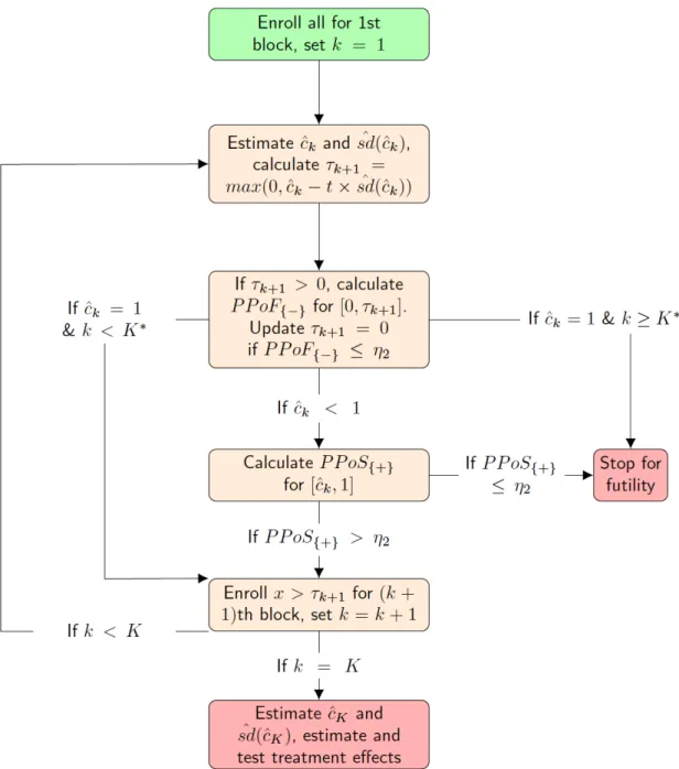
In Topic 3, we propose a group-sequential adaptive enrichment design, in which the optimal biomarker threshold is regularly updated using a grid search for maximizing utility, involving a trade off between the size of the positive population and the treatment effect in that population. Patients with a positive biomarker defined by the updated biomarker threshold are all enrolled and patients with a negative biomarker will be enrolled or excluded according to the Predictive Probability of Failure for such patients. Stopping for futility is also considered based on the Predictive Probability of Success for biomarker-positive patients. 2.3 Bayesian methods and Missing Data Approaches
As in Song et al. (2009), conditional on the sample size and the first-stage sample, the individual (Xi,Yi) falling into kth stratum is selected for observation, giving Ri = 1
(Ri = 0 if Xi is not observed), with prespecified probability pk. Then we have a ’missing at
random (MAR)‘ structure: P r(Ri = 1|Yi) = K Q
k=1
pI{Yi∈Ck}
k . Thus, we can cast the two-stage
outcome-dependent sampling design into a general missing-data framework.
parameters of the missing-data mechanism are distinct from the parameters of the sampling model, i.e., the joint distribution of (Xi,Yi), are said to be ignorable missing. In these cases,
the missing-data mechanism can be ignored in making likelihood-based inferences about the parameters of the sampling model.
2.3.1 Bayesian MCMC
Bayesian methods is increasingly popular for use in social science and other application areas where the data are observations from an informative sample. An informative sampling design leads to inclusion probabilities that are correlated with the response variable of interest. Model inference performed on the observed sample taken from the population will be biased for the population generative model under informative sampling since the balance of information in the sample data is different from that for the population.
Chen (2004) mentioned that the parametric modeling approach has two disadvantages: (1) parametric covariate models are not robust to model misspecification, and thus a large bias may be introduced into the regression parameter estimator if the model is misspecified, and (2) computing the estimates of the regression para meter involves intractable integrations when either a nonlinear regression model or a nonnormal covariate model is involved.
However, Bayesian methods can overcome the first disadvantage by estimating the prior according to historical data or SRS data in our design and employing noninformative hyperprior if needed. Moreover, Bayesian methods can model nonnormal covariate models with no limitation.
The Bayesian MCMC methods was first proposed by Tanner and Wong (1987), in which the missing data were sampled iteratively from their conditional distributions. Let Xmis and
Xobs be the missing values and observed values respectively. Letθ be the parameters of the
sampling model. Then at each iteration t sample,
Xmis(t) ∼ p(Xmis|Xobs, θ(t−1))
θ(t) ∼ p(θ|Xobs, X
(t)
After convergence of the Gibbs sampler, we can treat sampled values of θ as draws from their marginal posterior distributionp(θ|Xobs). Inferences about θ can then be made using
the posterior samples.
Fully Bayesian methods for missing covariate data in regression problems are quite straightforward conceptually. To carry out inference for (β, α)based on the observed data posterior, given by
p(β, α|Y, Xobs)∝ n Y
i=1
( Z
Xmis,i
p(Yi|β, Xobs,i, Xmis,i)×p(Xmis,i|Xobs,iα)dXmis,i )!
(2.21)
we do the following:
1. Specify the covariate distributionp(Xmis,i|Xobs,i, α).
2. Specify a joint distribution for(β, α), in which (β, α) can be taken independent or dependent a priori. Also, the joint prior distribution can be proper or improper.
3. To sample from the posterior p(β, α|Y, Xobs), do the following:
– Sample fromp(β|Y, Xobs, α, Xmis)
– Sample fromp(α|Y, Xobs, β, Xmis)
– Sample fromp(Xmis|Y, Xobs, β, α)
If the observed data likelihood can be factored, then the efficiency of the Gibbs sampler can be increased by sampling the parameters according to that factorization.
have missing covariates. Further, denote the ith row of X0 byx
0
0i = (x0i1, ..., x0ip) and the
ith component of Y0 by Y0i. The joint power prior for (β, α)takes the form
π(β, α|a0, D0,obs)∝π∗(β, α|a0, D0,obs)π0(β, α) (2.22)
where
π∗(β, α|a0, D0,obs) = n0
Y
i=1
Z
X0,mis,i
(p(Y0i|β, X0,obs,i, X0,mis,i)a0p(x01i|α1)a0i1
×
p−1
Y
j=1
p(x0i,p−j+1|x0i1, ..., x0i,p−j, αp−j+1)a0i,p−j+1)dX0,mis,i
(2.23)
p(y0i|β, X0,obs,i, X0,mis,i) is the complete-data likelihood for the ith subject with the current
data D = (n, Y, X) replaced by the historical data D0, the joint covariate distribution in the above equation is the same as for the current data with D replaced by D0, and D0,obs = (n0, Y0, X0,obs) is the observed historical data.
The termπ0(β, α)is called the “initial prior” of(β, α), that is, π0(β, α)is the prior of(β, α) before observing the historical data. The quantity 0 < a0 <1 is a scalar prior parameter that weights the complete-data likelihood of the historical data relative to the current study. To properly weight the historical complete-data likelihood, let a0i,p−j+1 =a0 if X0i,p−j+1 is observed anda0i,p−j+1 = 1ifX0i,p−j+1 is missing,i= 1, ..., n,j = 1, ..., p. The prior parameter a0 can be interpreted as a precision parameter that controls the heaviness of the tails of the joint prior for(β, α). It is reasonable to take a vague prior for π0(.), and take β and α to be independent at this stage. The parameter a0 can be taken as fixed or random. When a0 is taken to be random, a beta prior is a reasonable choice Ibrahim et al. (2002).
missing data, parameter estimation can become too computationally intensive and inefficient. The proposed parametric modeling scheme for the distribution of the covariates Ibrahim et al. (2002) as a sequence of one-dimensional conditional distributions is quite useful in the Bayesian context since it greatly reduces the number of nuisance parameters that have to be specified, thus greatly easing the computational strategies.
Ibrahim et al. (2005) reviewed four common approaches for inference in generalized linear models (GLMs) with missing covariate data: maximum likelihood (ML), multiple imputation (MI), fully Bayesian (FB), and weighted estimating equations (WEEs). They used a real dataset and a detailed simulation study to compare the four methods. In comparing the ML, MI, FB, and WEE methods based on correctly specified covariate models, ML, MI, and FB were quite comparable to each other, whereas WEE performed slightly worse.
For the non-ignorable informativeness, one approach is to account for it by parameterizing the sampling design into the Bayesian model (Little, 2004). The Bayesian approach is well equipped to handle complex design features such as clustering through random cluster models (Scott and Smith, 1969), stratification through covariates that distinguish strata, nonresponse (Little, 1982; Rubin, 1987; Little and Rubin, 1986) and response errors. Moreover, the Bayesian approach may yield better inferences for small sample problems where exact frequentist solutions are not available, by propagating error in estimating parameters (Little, 2004).
The specification of the joint distribution of the data and the missing data mechanism mainly focuses on two types of models: selection models and pattern-mixture models (Glynn et al., 1986; Little, 1993).
As in a general missing-data regression problem, let W= (Wij)denote a rectangular data
set involving the response and all covariates, wherei= 1, ..., n for individuals and j = 1, ..., k for variables. We partition W into observed and missing values, W= (Wobs,Wmis). Let
R= (Rij)be the missing-data indicator for W, with value 1 if Wij is observed and 0 if Wij
full data is
f(W, R|β, θ) = f(Wobs, Wmis, R|β, θ) (2.24)
Selection models specify the joint distribution of Wi and Ri through models for the
marginal distribution of Wi and the conditional distribution of Ri given Wi:
f(Wobs, Wmis, R|γ, φ) =f(Wobs, Wmis|γ)fR|W(R|Wobs, Wmis, φ) (2.25)
An advantage of the selection model factorization is that it includes the model of interest term f(Wobs, Wmis|γ)directly.
On the other hand, pattern-mixture models specify the marginal distribution of Ri and
the conditional distribution of Wi given Ri:
f(Wobs, Wmis, R|δ, ν) =f(R|δ)f W|R(Wobs, Wmis|R, ν) (2.26)
The pattern mixture model corresponds more directly to what is actually observed, i.e., the distribution of the data within subgroups having different missing data patterns.
a stratified sampling design). These approaches are designed for inference about simple mean and total statistics, rather than inference for parameters that characterize an analyst-specified population model that is the focus for our proposed method.
Savitsky et al. (2016) constructed a sampling-weighted pseudo posterior distribution by exponentiating each unit likelihood contribution, under the analyst-specified model, by its sampling weight, to produce, p(yi|δi = 1, λ)wi. Exponentiating by the sampling
weight, wi ∝1/πi, constructs the pseudo likelihood used to estimate the pseudo posterior
when convolved with the prior distributions for model parameters, λ. Savitsky et al. (2016) demonstrate that estimation of the model parameters from the pseudo posterior distribution is asymptotically unbiased. This approach provides a “plug-in” approximation to the population likelihood (forn observations), in that the sampling inclusion probabilities, πi, are assumed
fixed.
2.3.2 Other Missing Data Approaches
Besides Bayesian method, in this subsection, we briefly review other missing data ap-proaches.
The EM algorithm
Dempster et al. (1977) presented a general approach to iterative computation of maximum-likelihood estimates when the observations can be viewed as in complete data, which was named EM algorithm since each iteration consists of an expectation step followed by a maximization step. They considered two sample space Y and X and a many-one mapping F from X to Y. The observed datay are a realization from Y and the corresponding x in
X is not observed directly, but only indirectly to lie in F−1(y), the subset of X determined byy =F(x), wherey is the observed data.
Dempster et al. (1977) postulated a family of sampling densities f(x|φ) depending on parameters φ and derive its corrsponding family of sampling densities g(y|φ) as
g(y|φ) = Z
−
The EM algorithm aims to find a value of φ that maximizesg(y|φ) given an observedy, while making essential use of f(x|φ). Each iteration includes two steps: the expectation step (E-step) uses current estimate of the parameter to find the expectation of complete data and the maximization step (M-step) uses the updated data from the E-step to find a maximum likelihood estimate of the parameter.
Ibrahim (1990) examined incomplete data for the class of generalized linear models (GLM) with discrete covariates, in which incompleteness is due to partially missing covariates on some observations. Ibrahim (1990) showed that under some very general conditions, the E-step of the EM algorithm can be written as a weighted complete data log-likelihood for any GLM when the unobserved covariates are assumed to come from a discrete distribution with finite range. Thus, it allows for a straightforward maximization in the M step, which leads to maximum likelihood estimates for the parameter.
Imputation method
Imputation is filling in missing data with plausible values. In order to deal with the problem of increased noise due to imputation, Rubin (1987) developed the multiple imputation for averaging the outcomes across multiple imputed data sets to account for this.
Assume Q is statistic of interest, which can be the expectation and variance of θ that can be estimated by (Xobs, Xmis). First, generate m completed data sets, X
(i)
com = (Xobs, X
(i)
mis),
where i = 1, ..., m and Xmis(i) is randomly drawn from pre-selected predictive distribution p(Xmis|Xobs). The, Qˆ(i), and its variance, Ui, can be calculated by X
(i)
com. We compute the
following quantities,
¯
Q =
Pm i=1Qˆi
m
¯
U =
Pm i=1Uˆi
m
B =
Pm
i=1( ˆQi−Q¯)2
m−1