Detection of incomplete enclosures of rectangular shape in remotely sensed
images
Igor Zingman, Dietmar Saupe
Computer and Information Science, University of Konstanz
Germany
Karsten Lambers
IADK, University of Bamberg
Germany
Abstract
We develop an approach for detection of ruins of live-stock enclosures in alpine areas captured by high-resolution remotely sensed images. These structures are usually of approximately rectangular shape and appear in images as faint fragmented contours in complex background. We ad-dress this problem by introducing a new rectangularity fea-ture that quantifies the degree of alignment of an optimal subset of extracted linear segments with a contour of rect-angular shape. The rectrect-angularity feature has high values not only for perfect enclosures, but also for broken ones with distorted angles, fragmented walls, or even a com-pletely missing wall. However, it has zero value for spu-rious structures with less than three sides of a perceivable rectangle. Performance analysis using large imagery of an alpine environment is provided. We show how the detection performance can be improved by learning from only a few representative examples and a large number of negatives.
1. Introduction
We address the problem of detecting remains of man-made enclosures used to hold livestock in grassland of mountainous regions. The livestock enclosures (LE) are of special archaeological interest because they offer important insights into historical development of alpine pastoralism. Their automated spotting was questioned in a recent ar-chaeological project [18]. Examples of such enclosures are shown in Fig. 1. These structures are usually composed of linear walls that may be heavily ruined. The most common shape of LE resembles a rectangular contour with greatly varying size and aspect ratio. Rectangle angles may deviate from right angles, and rectangle sides may be fragmented. The angle between adjacent fragments of the same (broken) side may deviate from 180 degrees. Moreover, the rectan-gular contours are sometimes incomplete such that even an entire side may be missing.
Figure 1. Livestock enclosures (LE) in alpine environment
We use satellite and aerial images of 0.5m resolution where the width of linear walls does not exceed two pixels. The ruined walls are of low height, which results in low con-trast linear features in the images. The spectral properties of LE are similar to the spectral properties of the surrounding terrain, rocks, and other irrelevant objects. The first row of Fig. 5 shows a satellite and an aerial image with structures corresponding to the LE shown in Fig. 1. Nearby irrele-vant structures, such as rivers, trails, or rocks, are often of similar or higher contrast either due to larger size (e.g. big rocks) or distinctive spectral properties (e.g. rivers). Detec-tion of such faint structures in a complex terrain is a chal-lenging task. Even the detection of easily modeled circular soil structures [32] had very limited success due to their low contrast and complex terrain. Only few examples of LE are available in our case, which presents another difficulty mak-ing most approaches that learn from the data inappropriate. Because of these difficulties, commonly used methods for rectangle detection are hardly applicable.
1.1. Related work
Detection of rectangular structures has previously been addressed in different contexts. Examples are detection of buildings in remotely sensed images [24, 19, 14, 3, 12, 15, 1, 31, 30, 23, 26], traffic signs [21, 13, 22], and particles of a rectangular shape in cryo-electron microscopy images [36, 35]. The methods used were based on Markov Random Fields [15, 21], Marked Point Processes [1, 26], search on a graph [14, 38], Hough Transform and other voting schemes [3, 12, 36, 13, 22], template matching [25], aggregation of local features [1, 23, 31], and heuristic rules [19].
Most techniques for detection of rectangular structures dealt with buildings in remotely sensed images. For exam-ple, in the graph-based approach [14], a search for cycles was used to generate building hypotheses. The search was accompanied by an extensive set of rules and thresholds, which limits the robustness of the approach.
Markov Random Fields (MRF) were used in [15] to de-lineate buildings. More recently, a similar approach was used in [21] for detection of traffic signs in color images. The approach is sensitive to inaccuracy of extracted edges and cannot detect incomplete rectangles, as it requires the presence of all four sides of a rectangular structure. The marked point processes (MPP) [4] recently became popular for extraction of various structures in remotely sensed im-ages, including buildings (e.g. in [1, 26]). The MPP proved to be very powerful when applied to real data. However, these stochastic methods are still computationally expen-sive. Similarly to the MRF, they may not converge to a globally optimal solution and usually need careful tuning of a large number of parameters. Attempts have recently been made to address some of these problems, which are crucial for the analysis of large images. In [33] substantial improvements in performance have been achieved for the extraction of line networks (roads and rivers). In this work also the potential of GPUs was efficiently exploited.
An approach for detection of rectangular contours based on the Hough transform was developed in [12]. The ap-proach relies on certain strict geometrical rules making it not suitable for detection of fragmented or incomplete struc-tures. It may also result in detection of rectilinear configu-rations that cannot form a rectangular contour. Detection of such configurations is prevented in our approach by adding a convexity constraint.
In [31] a set of local features that carried local corner in-formation were used to produce a probability map of build-ing rooftops. Unfortunately, in the case of fragmented en-closures corners are not reliable features. Moreover, local features in general do not suffice in the case of faint con-tours appearing in a cluttered background. A more global description that takes into account spatial relations between local features is necessary. For example, in [1, 23] the gra-dient orientation density function (GODF) was computed
from image gradients. A correlation of this function with a mixture of two Gaussians having mean values separated by ninety degrees served as a GODF-based feature indicating the presence of buildings.
Although there is a variety of methods developed for building detection, they are not applicable to our task be-cause buildings are much more salient structures. In con-trast to building rooftops, walls of ruined livestock enclo-sures are narrow and are of low hight (low contrast fea-tures), may be highly fragmented, or even completely miss-ing. Higher contrast irrelevant structures may appear inside or outside of rectangular structures in the immediate neigh-borhood. Various cues (rooftop color, shadows, 3D cues etc.) usually employed in building detection algorithms are not available.
1.2. Overview of our approach
Our approach relies on the basic detection scheme, which includes localization of candidate points, we pre-sented in [38]. A binary map of edges accompanied by angle information is computed first. Linear segments are then found and modeled by a few parameters with the use of a local Hough transform. An undirected graph is con-structed, nodes of which correspond to linear segments and graph edges encode spatial relations between linear seg-ments. Particularly, we use angle and convexity properties to encode spatial relations. Due to the construction of the graph, its maximal cliques correspond to valid configura-tions of linear segments. The valid configuraconfigura-tions are then ranked by a new rectangularity measure that encodes the goodness of grouping the segments into a rectangular struc-ture (Sec. 2.3). In contrast to [38], the new rectangularity measure does not rely on a heuristic partitioning of the set of linear segments into four subsets. Hard decisions are soft-ened. Configurations better matching the rules result in a higher rectangularity measure. The rectangularity feature is defined as the maximal rectangularity measure of all valid configurations (Sec. 2.4). In practice, the number of cor-responding maximal cliques within the analysis window is low, allowing exact and efficient maximization. The result-ing rectangularity feature captures the presence of Π-like structures and is robust to their fragmentation.
discuss future directions.
2. Measuring structure rectangularity
We introduce a rectangularity featurefRcomputed from a set of linear segmentsW ={Si, i= 1, ..., m}that were extracted from a gray-scale image.
2.1. Grouping edge points into linear segments
In Sec. 3.1 we provide details on approaches we used to extract ridges and valleys (bar edges) and to detect candi-date locations. Given a candicandi-date location and edge points accompanied by estimated orientations we extract and pa-rameterize linear segments, each of which is a group of aligned edge points. Linear segments are represented by a triple of parameters(θ, r, l)found by the use of a local Hough transform centered at the candidate points. We use the Hough transform in the form introduced in [6], where a line is defined by the orientation θof the normal and a distancerfrom the origin
r=xcosθ+ysinθ. (1)
The spatial coordinates of an edge point are x, y, θ ∈
[0,360), and r ∈ (0,∞). A peak at(θ, r)in the Hough plane corresponds to a line. The peaks are detected as re-gional maxima in the Hough plane that was discretized with
Δθ= 3◦andΔr= 1pixel. The detected line corresponds
to either a single connected linear segment S, or to sev-eral aligned connected components. In the latter case, the connected components with gaps smaller than a predefined threshold (3 pixels in our experiments) are considered a sin-gle linear segment (see the segmentSjin Fig. 2), otherwise they are considered separate linear segments. This was not allowed in [38], where Hough lines always corresponded to a single linear segment (connected or fragmented), which restricted the number of candidate configurations of linear segments. The parameterlin the triple(θ, r, l)is the num-ber of points that belong to the linear segment. To better relate the parameterlto the length and avoid its dependence on the width of the extracted edges, we perform their thin-ning [17] prior to clustering in a Hough plane.
Since edges were extracted together with their orienta-tions,rcan be directly computed for each edge point(x, y) using Eq. (1). Thus, each edge point votes for a single point in the(θ, r)plane instead of voting for a curve as suggested in [6]. This idea, which was used already in [7] for cluster-ing of short ridge features, considerably eases extraction of meaningful peaks in the Hough plane.
2.2. Valid configurations of linear segments
Below we define a valid configuration of linear segments
C ⊆ W that can be a part of a rectangular structure. We require anglesβk,jbetween linear segmentsSk,Sj ∈Cof
the valid configuration to be close to either zero, 180◦, or right angles. An angle toleranceαwill be set to control the strictness of the angle constraint. We defineβk,jas
βk,j= min(|θSk−θSj|,360− |θSk−θSj|). (2)
Note thatβj,k =βk,jandβ ∈[0,180], sinceθ∈[0,360). The angle constraint alone does not suffice to restrict config-urations to be perceptually close to rectangles or rectangle parts. We therefore define a second constraint that requires the valid configuration to be nearly convex in the sense that extension of all linear segments of the configuration can form an nearly convex contour. The convexity tolerance
t will be defined to control the strictness of the convexity constraint. For a convex configuration of linear segments it is required that a half plane generated by each segment in-cludes all other segments of the configuration. Additionally, we require that all these half planes contain the candidate point around which we search for a rectangular structure. Pair-wise convexity constraints suffice to verify the convex-ity of a configuration containing the given candidate point. We define the pair-wise convexity measureτ for a pair of linear segmentsSk,Sj, each with corresponding attributes of sizelS, orientationθS, and distancerS to the candidate
pointp0, as
τk,j = max(˜τk,j,τ˜j,k), (3)
˜
τk,j = l1 j
p∈Sj
H((p−p0)T·n
k−rk), (4)
wherenk = (cosθk,sinθk)T is the unit normal ofSkand
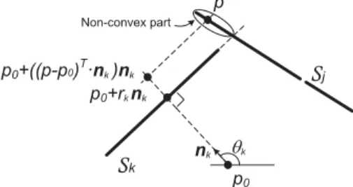
H(u)is an indicator function equal one foru >0and zero otherwise. τ˜k,j measures the relative number of points in the segmentSj that are behind the segmentSk, relative to the given candidate pointp0 as illustrated in Fig. 2. Note thatτ ∈[0,1], andτk,j=τj,k, whileτ˜k,j= ˜τj,k.
6M
S
S
1RQFRQYH[ SDUW
SUNQN
TN
6N
SSS7āQNQN
QN
Figure 2. The fraction of pointspofSjthat violates the convexity constraint relative toSkandp0is given byτ˜k,j. Note that linear segments can be fragmented having small gaps as inSj.
Definition 1. Letα ∈[0,45], t ∈[0,1], a candidate point
p0, and a configuration Cof linear segments be given. If for all pairsSk,Sj ∈ C,j = k, one of the inequalities of the angle constraint
and the convexity constraint
τk,j≤t (6)
both hold, thenC is called a (t,α)-valid configuration lo-cated aroundp0, and denoted byCt,αp0.
For the sake of brevity, we usually omit the indicest,
αand the reference pointp0, mentioning thatCis a valid configuration. Valid configurations include not only perfect rectangles, but also convex polygons or their parts with an-gles around either 90 or 180 degrees. This is important in practice since approximately rectangular structures are bet-ter modeled by such polygons rather than by perfect rectan-gles.
2.3. Rectangularity measure of a valid configuration
A couple of poorly aligned short segments can be a valid configuration as far as the tolerances t, αallow. There is a need to rank valid configurations according to their simi-larity to a canonical rectangle. To find and rank valid con-figurations we construct an undirected graphGw from the given setWof linear segments in a window centered at a candidate pointp0. The graphGw has nodesj = 1, .., m corresponding to the segmentsS1, ..,Sm ∈W. Each node
jis attributed by a triple of parameters(θj, rj, lj), i.e. ori-entation, distance to the reference pointp0, and size of the linear segment. An edge{k, j}is attributed with the angle
βk,j and the pair-wise convexityτk,j of the corresponding pair of segmentsSk,Sj. An edge{k, j}is included in the graph Gw if βk,j andτk,j satisfy the constraints in Eqs. (5, 6). This attributed graph encodes properties of linear segments and their spatial relationships. Due to the graph construction and Definition 1, valid configurationsC corre-spond to fully connected subgraphsGc, also called cliques, of the graphGw.
Below we introduce the new rectangularity measure
ρ(Gc)that ranks a cliqueGccorresponding to a valid
con-figurationC⊆W. We define the measure with the follow-ing properties in mind. The rectangularity measure shall yield higher values for configurations with
1. higher degree of convexity given by lower values of the convexity measureτ
2. higher degree of angle alignments given by anglesβ
3. longer linear segments given by largerl.
In addition, the proposed rectangularity measure shall
4. have the increasing property ρ(Gc1) ≤ ρ(Gc2) for
Gc
1⊆Gc2. Thus, the rectangularity measure of a larger encompassing clique has a higher value
5. yield a zero value for configurations of linear segments with less than three sides of a rectangle.
We define the rectangularity measure of a graph cliqueGc in terms of sums over its undirected edges{k, j} ∈Ec
ρ(Gc) =
⎛ ⎝
⎛
⎝
{k, j} ∈Ec
lkljf90(βk,j)fcv(τk,j)
⎞
⎠×
⎛
⎝
{k, j} ∈Ec
lkljf180(βk,j)fcv(τk,j)
⎞ ⎠
⎞ ⎠ 1 4
, (7)
wheref90,f180,andfcvare mode functions depicted in Fig. 3.f90andf180equal zero for anglesβthat deviate from the mode center larger than the angle tolerance α. fcv equals zero for the convexity measureτ larger than the convexity tolerancet. In our experiments we usedα = 35◦andt =
0.3. The exact definition of the mode function is not critical and is not given here due to space constraints.
0 45 90 135 180 0.5
1 f90
f 180
0 0.3 0.6 0.9 0.5
1
f cv
Figure 3. Functionsf90(left figure, solid blue curve),f180(left
fig-ure, dashed red curve), andfcv(right figure) used in the definition of the rectangularity measure in Eq. (7).
The first factor of ρ(Gc)in Eq. (7) yields a non-zero value only if the valid configurationCcontains at least one pair of approximately perpendicular linear segments that fulfill the convexity constraint in Eq. (6). The second factor is non-zero only if the valid configuration contains at least one pair of approximately parallel linear segments1. The product of these two factors is non-zero only if the valid configurationCcontains at least one pair of parallel and one pair of perpendicular linear segments. The angles between linear segments of these parallel and perpendicular pairs are restricted to be approximately 0, 180, or 90 degrees sinceC is a valid configuration with linear segments constrained by Eq. (5). Thus, a non-zero rectangularity measure insures a valid configurationCcontaining at least one triple of seg-ments arranged in a Π-like structure, as stated in property 5 above. This property allows suppression of a large num-ber of configurations originating from clutter (e.g. lines, corners, junctions etc.). It is easy to verify that the other four properties above are also satisfied by the rectangularity measure in Eq. (7).
1fcvin the second term has only a small impact on results. It reduces
Note that the rectangularity measure is a function of graph node and edge attributes and does not require explicit partitioning of a valid configuration of linear segments into four subsets corresponding to four sides of a hypothesized rectangle as required in [38].
2.4. Rectangularity feature
Given a set of linear segmentsW in an analysis win-dow, we define the rectangularity featurefRof the corre-sponding graphGw using the rectangularity measure of its cliquesGc. Let us denote the set of cliques asK(Gw). The rectangularity feature ofGwis defined as
fR(Gw) = max
Gc∈K(Gw)ρ(G
c). (8)
The corresponding optimal clique is
Gc
opt= argmax
Gc∈K(Gw)ρ(G
c). (9)
Due to the increasing property ofρ(the fourth property of the rectangularity measure stated in Sec. 2.3), the maximum can be searched over the set of maximal cliques2only, de-noted here byM(Gw)
fR(Gw) =ρ(Gc
opt) = max
Gc∈M(Gw)ρ(G
c). (10)
Since the set of maximal cliques M(Gw) ⊆ K(Gw) is much smaller than the set of graph cliques K(Gw), the number of times the rectangularity measureρneeds to be evaluated in Eq. (10) is considerably reduced in compari-son to Eq. (8). Since, in addition, there are efficient algo-rithms for the search of maximal cliques [2], computing the rectangularity feature is not computationally demanding.
Fig. 4 (left) shows an example of a given set W =
{S1,S2, ..,S6}of linear segments and the optimal config-urationCopt={S1,S2,S3,S5}in red, while Fig. 4 (right) shows the corresponding graphGw and the optimal max-imal clique Gcopt in red. There are two additional max-imal cliques Gc1 andGc2and corresponding valid config-urations C1 = {S2,S3,S4,S6},C2 = {S1,S2,S3,S4}. They, however, have lower rectangularity valuesρ(Gc1)<
ρ(Gc
opt), ρ(Gc2)< ρ(Gcopt).
2.5. Adjusted rectangularity feature
The rectangularity feature scales with the structure size having lower values for small structures. A detector based on such a feature is prone to dismiss small rectangles. On the other hand, false structures of a small size are more fre-quent. We, therefore, introduce an additional feature fS proportional to the structure size and learn a classifier from the available data in the two-dimensional feature space.
2Maximal cliques are cliques that are not contained in larger cliques.
6
6
6 6
6
6
S
Figure 4. Left: A given setW = {S1,S2, ..,S6}of linear seg-ments around a candidate pointp0. Right: A graphGwfor the set of linear segments. We assume an angle toleranceαsuch that all angle constraints are satisfied. Several node pairs of the graph are not connected by an edge due to the convexity constraint, which is not satisfied for an assumed convexity tolerancet. The red nodes of the graph are the nodes of the optimal maximal cliqueGcopt. The corresponding valid configurationCoptis marked in red on
the left figure.
This may improve the trade-off between the sensitivity and the number of false detections in comparison to the one-dimensional case. We define the size of the structure, rep-resented by the optimal cliqueGcopt⊆Gw, as
fS(Gw) =
jljrj
jlj , (11)
where the sums are over all nodes of the optimal clique
Gc
opt.fSis computed as the weighted distance of the linear segments ofCopt from the corresponding candidate point, where the weights are segment sizes.
Since only a few positive examples are available in our case, a classification approach should be carefully chosen. The linear classifiers are favorable when there is a danger of overfitting the data due to a limited number of avail-able examples. They also are not computationally demand-ing. Simple linear classifiers may be powerful enough when used together with a few category-specific features as op-posed to the use of many generic features, [34]. We care-fully constructed such rectangularity and size features. The normalwof the separating hyperplane of a linear classifier can be found by means of the Fisher Linear Discriminant analysis (FLD). In this approach, the optimal direction is determined such that the data from two classes projected onwis maximally separated. The separation is measured by the squared distance between class means normalized by the sum of their variances [9, 7]. This approach results in a simple solution represented in terms of class means and covariance matrices. In our case, however, the number of positive examples is very limited and the covariance matrix cannot reliably be estimated.
between an arbitrary pointyand the distributionXof neg-atives, both projected to the directionwand normalized by the standard deviation of the projected distribution by
Dw(y, X)≡
ExwTy−wTx
Ex[(wTx−wTμx)2]
= wT(y−μx)
wTC xw
,
(12) whereμxandCxare the mean and the covariance matrix of the distributionX, respectively. Next, we define the average signed distance between a set of points {yi, i = 1, ..., n} and the distributionX
¯
Dw({yi}, X)≡ n1 n
i=1
Dw(yi, X) = w T(¯y−μ
x)
wTCxw , (13)
wherey¯ = n1ni=1yi. We now define the optimal direc-tionw as the direction that maximizes the absolute value of the average signed distance between a set of points cor-responding to positive examples and the distribution of the dominant class of negativesX, i.e.
wopt≡argmax
w |
¯
Dw({yi}, X)|. (14)
From Eqs. (13, 14) we obtain
wopt= argmax
w
|wT(¯y−μ x)|
wTC xw
. (15)
It can be shown that
wopt=Cx−1(¯y−μx) (16)
is a solution of Eq. (15). The obtained direction wopt is similar to the one in the FLD analysis [7]. In contrast to the FLD solution, Eq. (16) includes the covariance matrix of the class of negatives only, preferring the solution in the direc-tion of the small variance of negatives. Negatives are well sampled in our problem and their covariance matrix can be robustly estimated. The positives are treated as determinis-tic points in the feature space and influence the solution only via their average. Literally, the average only weakly guides the solution showing were the novelties of our interest re-side. The samples ofXmay include outliers. Therefore, in Eq. (16) we use the robust Multivariate Trimming estimates of the mean and the covariance matrix [5].
Given the optimal hyperplane defined bywopt, samples with coordinates(fS, fR)in feature space can be character-ized by the adjusted rectangularity feature
ˆ
fR= (fSfR)wopt. (17)
Thereby, the adjusted rectangularity feature is an optimal linear combination of the rectangularity and size features. Note that this approach is not limited to two dimensional feature spaces, but directly extends to higher dimensions.
3. Experiments
We evaluate the discrimination ability of the introduced rectangularity features and provide comparison with the NMR measure in [38] and the GODF-based feature in [1] using our implementation, see Sec. 3.3.
3.1. Data used and preprocessing
In our experiments we used panchromatic images cap-tured by the GeoEye1 satellite and the red channel of Swiss Topo aerial images. Both types of images are at 0.5m res-olution. Nine examples of enclosures taken from aerial and satellite images were available for us. A large number of negative examples was generated from19000×10000pixel size satellite image of the Silvretta mountains, which corre-sponds to about48km2. The data stems from a recent ar-chaeological project in the Silvretta mountains [18].
We used the preprocessing flow as in [38]. Bar edges were extracted using the Morphological Feature Contrast based line detector [40, 39]. This technique extracts lin-ear features, while suppressing texture elements of cluttered background. We also experimented with other approaches [20, 10, 28], but these are either not sensitive enough to ex-tract faint edges of enclosures, or generate lots of clutter edges depending on the parameters used. The parameter-less line segment detector [11], which is known to provide robust results for a large range of images, misses faint edges of enclosures. Extraction of candidate points was carried out by sampling the skeleton points of a complementary bi-nary map of detected bar edges [38]. The second row of Fig. 5 shows examples of maps of bar edges and candidate points for the corresponding images in the first row. Along with the skeleton, we computed the distance transform of the set of bar edges. The values of the distance transform at the candidate points were used to adaptively define the sizes of an analysis window. We discarded all candidate points having a distance smaller than 10 or greater than 90 pixels, which limits the distances between opposite walls of the structures. High contrast texture regions were fil-tered out using the Morphological Texture Contrast descrip-tor [40, 39, 37] thresholded with the Otsu method [27]. This filters out urban areas, forests, rocky mountains, and other high contrast texture regions, but preserves individual struc-tures.
3.2. Measuring discrimination power
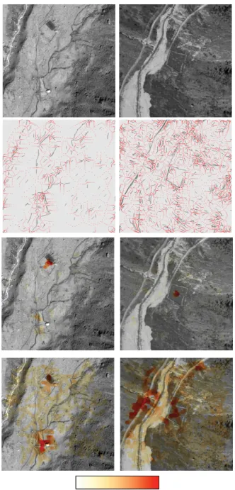
Figure 5. First row: 600×600satellite ( cGeoEye 2011) and aerial (SWISSTOPO) images of 0.5m resolution with structures corresponding to livestock enclosures in Fig. 1. Second row: Bar edges (black) and candidate points (red) generated from the im-ages in the first row. Third row: The rectangularity feature com-puted at each candidate point and visualized by a colored disk. Fourth row: The GODF-based feature. Color saturation increases and hue is changing from yellow to red for growing values of the features in accordance with the color bar in the bottom.
possible measure of this ability is the minimal number of FP detected with the threshold that insuresT P R ≥ ξ, where
ξ is the predefined rate of true positives3. We computed
F P forξ = 1, denoted in the following byF P100. This was done by setting the detection threshold to the minimum value of the rectangularity feature computed for nine avail-able positives. Obviously, the threshold used to obtain the detection rateT P R= 1on a small number of available ex-amples does not insure a detector with100%detection rate. However, it allows us to measure and compare the discrim-ination ability of the rectangularity features.
We also used an alternative measure of the discrimina-tion ability that is the area under receiver operating char-acteristic (ROC) curve. It is especially useful in the pres-ence of unbalanced classes [8, 16]. In contrast to F P100, the area under receiver operating characteristic (AUC) does not rely on a particular threshold and a corresponding oper-ating point on the ROC curve, but instead summarizes the detection performance for different values of the threshold.
3.3. The gradient orientation density function (GODF) based feature
The GODF-based feature was recently used in [1, 23] for detection of buildings. The GODF, denotedλ(θ), captures the distribution of orientations of intensity gradients. The correlation ofλ(θ)with a function having two modes sepa-rated by90◦served as a GODF-based featurefGindicating the presence of rectilinear structures. LetAbe the neigh-borhood around a candidate point and let us denote byg(p) the intensity gradient (the Prewitt operator was used) and byϕg(p)the gradient orientation atp. λ(θ)is computed as a weighted gradient orientation histogram with gradi-ent magnitudes g(p) as weights, and discrete orientation
θ∈[0,180), θ=kΔθ, wherek= 0,1,2, ...,
λ(θ) = 1
B
p∈A
g(p) I(θ, ϕg(p)). (18)
The discrimination stepΔθwas set to one. Bis a normal-izing constant such thatλ(θ)is a unit vector4, andI(θ, ϕ) is the indicator function that equals one ifϕ∈[θ, θ+ Δθ), and zero otherwise. The GODF-based featurefGat the can-didate point is then defined as a circular correlation of the orientation histogramλ(θ)with the functionfΔ90
fG= max ϑ∈[0,90)
θ
λ(θ)fΔ90((θ−ϑ)modulo180). (19)
fΔ90 is defined in the interval [0,180) and composed of modes separated by90◦. The shape of the modes was the same as for the modes off90andf180in Eq. (7).
3.4. Results
The rectangularity featurefR2 computed at the candidate points is visualized by colored disks in Fig. 5 (third row).
3This corresponds to the so-called Neyman-Pearson task [29]. 4This gave us better results than forB=
It was squared in order to visually better distinguish its low and high values. As expected, high values were obtained at positions of LE while zero or low values were obtained at most other candidate positions. Visually similar results are obtained with the NMR measure from [38]. We do not show the corresponding images here (see examples in [38]) due to space limitations. Less convincing results were obtained for the GODF-based featurefG8 in Fig. 5 (fourth row). The GODF-based feature was raised to the eighth power, since the second power did not suffice to visually distinguish its low and high values. One can see that the rectangularity feature map is much sparser than the GODF-based feature map. This is partially because the rectangularity feature has zero value for spurious structures with less than three sides, while the GODF-based feature may have only small non-zero values for such structures.
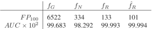
The quantitative measures of performance are summa-rized in Table 1. The structures were detected out of 403716 candidate positions in the19000×10000pixel image. The results show that the discrimination ability of the adjusted rectangularity featurefˆRis superior to the others. It allows reduction of FP by24%relatively tofR, which is in turn considerably better than the NMR measure in [38]. Though effective for building detection, the GODF-based feature turned out to be far worse for detecting faint enclosures in cluttered background. This feature is not useful when computed over large windows, where the relative number of points belonging to an enclosure is very low. Fig. 6 shows typical FP obtained for the rectangularity features. These FP were caused by streams and roads. The use of 3D data (e.g. LiDAR) would allow the discrimination of such FP.
Figure 6. Typical false positives (within color rectangles).
The experiments were carried out using Matlab on a ma-chine with an Intel Core i5 3.3 GHz processor. Generation of candidate locations and computation of the introduced rectangularity features took about two hours. Generation of the NMR measure and the GODF-based feature took about forty and ninety minutes, respectively.
4. Discussion and Conclusion
The introduced rectangularity and the adjusted (learnt) rectangularity features have shown good performance dis-criminating ruined enclosures from irrelevant structures and clutter in remotely sensed images. Due to the inherent
diffi-fG fN fR fˆR
F P100 6522 334 133 101
AUC×102 99.683 98.292 99.993 99.994
Table 1. Detection performance using the GODF-based featurefG
([1]), the normalized maximum rectangularity measurefN([38]),
the rectangularityfR, and the adjusted rectangularityfˆRfeatures.
culties of our problem, such a performance is hardly achiev-able with other approaches for detection of rectangular con-tours, nor with related approaches, e.g. for detection of buildings. As an example we have shown that the GODF-based feature used for detection of buildings (e.g. in [1]) re-veals a poor discrimination ability for our task. Note that we did not compare the rectangularity features with the whole approach developed in [1], because it is based on additional features not appropriate in the case of enclosures. Also, pa-rameters of the data model would be hard to estimate from only few available examples of enclosures. We have also tested other methods for building detection (e.g. [31, 12]) applied to detection of livestock enclosures. Unfortunately, these methods completely fail to detect the enclosures, pre-venting us from reporting the corresponding quantitative comparison.
In general, methods for building detection are not suit-able for our case because of considerably lower heights (related to low feature contrasts) and feature sizes (ruined walls versus building rooftops), and due to the absence of various cues (roof colors, roof homogeneity, shadows, 3D cues, etc.). Some walls or parts of them may be missing or may also be missed in the edge extraction (the width of lin-ear features does not exceed two pixels in images of 0.5m resolution). Various irrelevant structures (trails, streams, rocks etc.) with sizes or/and reflectance properties similar to those of enclosure walls may occasionally form rectilinear configurations. In contrast to enclosures, building rooftops are much more distinctive structures.
It is interesting to investigate the usefulness of the rectan-gularity features for detection of targets other than livestock enclosures. We believe, for example, that our approach may have comparative performance for detection of abandoned buildings or other architectural structures in rural or moun-tainous areas5. Building contours can be extracted with standard edge detection algorithms and used as an input for our approach. Note that, while building detection problem can be transformed to detection of enclosures6, it does not work in the opposite direction. We also plan to incorporate additional features and apply the FLD-based detector to vast alpine areas in order to spot unknown livestock enclosures.
5In urban areas our approach is likely to be too sensitive. Walls of
adjacent buildings may cause a large number of false detections within urban areas.
References
[1] C. Benedek, X. Descombes, and J. Zerubia. Building devel-opment monitoring in multitemporal remotely sensed image pairs with stochastic birth-death dynamics.IEEE Trans. Pat-tern Anal. Mach. Intell., 34(1):33–50, 2012.
[2] C. Bron and J. Kerbosch. Algorithm 457: finding all cliques of an undirected graph. Commun. ACM, 16(9):575–577, Sept. 1973.
[3] A. Croitoru and Y. Doytsher. Right-angle rooftop polygon extraction in regularised urban areas: Cutting the corners.
The Photogrammetric Record, 19(108):311–341, 2004. [4] X. Descombes and J. Zerubia. Marked point process in
im-age analysis. Signal Processing Magazine, IEEE, 19(5):77– 84, 2002.
[5] S. J. Devlin, R. Gnanadesikan, and J. R. Kettenring. Ro-bust estimation of dispersion matrices and principal com-ponents. Journal of the American Statistical Association, 76(374):354–362, 1981.
[6] R. O. Duda and P. E. Hart. Use of the Hough transforma-tion to detect lines and curves in pictures. Commun. ACM, 15(1):11–15, Jan. 1972.
[7] R. O. Duda and P. E. Hart.Pattern Classification and Scene Analysis. John Willey & Sons, 1973.
[8] T. Fawcett. An introduction to ROC analysis. Pattern Recogn. Lett., 27(8):861–874, June 2006.
[9] K. Fukunaga.Introduction to Statistical Pattern Recognition. Academic Press., 1990.
[10] C. Grigorescu, N. Petkov, and M. Westenberg. Contour and boundary detection improved by surround suppression of texture edges. Image and Vision Computing, 22:609 – 622, 2004.
[11] R. Grompone von Gioi, J. Jakubowicz, J.-M. Morel, and G. Randall. LSD: A fast line segment detector with a false detection control. IEEE Trans. Pattern Anal. Mach. Intell., 32(4):722–732, Apr. 2010.
[12] C. R. Jung and R. Schramm. Rectangle detection based on a windowed Hough transform. InProceedings of the Com-puter Graphics and Image Processing (SIBGRAPI), XVII Brazilian Symposium, pages 113–120, 2004.
[13] C. G. Keller, C. Sprunk, C. Bahlmann, J. Giebel, and G. Baratoff. Real-time recognition of US speed signs. In
Intelligent Vehicles Symposium, pages 518–523. IEEE, 2008. [14] T. Kim and J.-P. Muller. Development of a graph-based approach for building detection. Image Vision Comput., 17(1):3–14, 1999.
[15] S. Krishnamachari and R. Chellappa. Delineating buildings by grouping lines with MRFS.IEEE Transactions on Image Processing, 5(1):164–168, 1996.
[16] W. J. Krzanowski and D. J. Hand.ROC Curves for Continu-ous Data. Chapman & Hall/CRC, 2009.
[17] L. Lam, S.-W. Lee, and C. Y. Suen. Thinning methodologies-a comprehensive survey.IEEE Transactions on Pattern Anal-ysis and Machine Intelligence, 14(9):869 – 885, 1992. p.879. [18] K. Lambers and I. Zingman. Towards detection of archae-ological objects in high-resolution remotely sensed images:
the Silvretta case study. In G. Earl et al., editors, Archaeol-ogy in the digital era (e-papers). Proc. of Computer Applica-tions and Quantitative Methods in Archaeology, volume II, pages 781–791, Southampton, UK, March 2012. Amsterdam University Press.
[19] C. Lin and R. Nevatia. Building detection and description from a single intensity image. Computer Vision and Image Understanding, 72(2):101–121, 1998.
[20] T. Lindeberg. Edge detection and ridge detection with au-tomatic scale selection. International Journal of Computer Vision, 30(2):117–156, 1998.
[21] Y. Liu, T. Ikenaga, and S. Goto. An MRF model-based ap-proach to the detection of rectangular shape objects in color images. Signal Processing, 87(11):2649–2658, 2007. [22] G. B. Loy and N. M. Barnes. Fast shape-based road sign
detection for a driver assistance system. In2004 IEEE/RSJ International Conference on Intelligent Robots and Systems, Sendai, Japan, pages 70–75, 2004.
[23] A. Manno-Kovacs and T. Sziranyi. Multidirectional Build-ing Detection in Aerial Images Without Shape Templates. IS-PRS - International Archives of the Photogrammetry, Remote Sensing and Spatial Information Sciences, (1):010000–232, May 2013.
[24] H. Mayer. Automatic object extraction from aerial imagery -a survey focusing on buildings.Computer Vision and Image Understanding, 74(2):138–149, 1999.
[25] H. Moon, R. Chellappa, and A. Rosenfeld. Optimal edge-based shape detection. IEEE Transactions on Image Pro-cessing, 11(11):1209–1227, 2002.
[26] M. Ortner, X. Descombes, and J. Zerubia. A marked point process of rectangles and segments for automatic analysis of digital elevation models. Pattern Analysis and Machine Intelligence, IEEE Transactions on, 30(1):105–119, 2008. [27] N. Otsu. A Threshold Selection Method from Gray-level
Histograms. IEEE Transactions on Systems, Man and Cy-bernetics, 9:62–66, Jan. 1979.
[28] G. Papari and N. Petkov. An improved model for sur-round suppression by steerable filters and multilevel inhibi-tion with applicainhibi-tion to contour detecinhibi-tion. Pattern Recogni-tion, 44:1999 – 2007, 2011.
[29] M. I. Schlesinger and V. Hlavac. Ten lectures on statistical and structural pattern recognition. Springer, 2002. [30] B. Sirmacek and C. Unsalan. Urban-area and building
detec-tion using SIFT keypoints and graph theory. IEEE T. Geo-science and Remote Sensing, 47(4):1156–1167, 2009. [31] B. Sirmacek and C. Unsalan. A probabilistic framework to
detect buildings in aerial and satellite images. IEEE Tran. Geoscience and Remote Sensing, 49(1-1):211–221, 2011. [32] Ø. D. Trier, S. Ø. Larsen, and R. Solberg. Automatic
detec-tion of circular structures in high-resoludetec-tion satellite images of agricultural land. Archaeological Prospection, 16:1–15, 2009.
[33] Y. Verdie and F. Lafarge. Detecting parametric objects in large scenes by Monte Carlo sampling.International Journal of Computer Vision, 106(1):57–75, 2014.
International Conference on Computer Vision, pages 281– 288 vol.1, Oct 2003.
[35] Z. Yu and C. Bajaj. Detecting circular and rectangular parti-cles based on geometric feature detection in electron micro-graphs. Journal of Structural Biology, 145(12):168 – 180, 2004.
[36] Y. Zhu, B. Carragher, F. Mouche, and C. S. Potter. Automatic particle detection through efficient hough transforms. IEEE Trans. Med. Imaging, 22(9):1053–1062, 2003.
[37] I. Zingman, D. Saupe, and K. Lambers. Morphological op-erators for segmentation of high contrast textured regions in remotely sensed imagery. In Proc. of the IEEE Int. Geo-science and Remote Sensing Symposium, pages 3451–3454, Munich, Germany, July 2012.
[38] I. Zingman, D. Saupe, and K. Lambers. Automated search for livestock enclosures of rectangular shape in remotely sensed imagery. In L. Bruzzone, editor, Proc. SPIE, Im-age and Signal Processing for Remote Sensing XIX, volume 8892, pages 88920F–1 – 88920F–11, Dresden, Germany, 2013.
[39] I. Zingman, D. Saupe, and K. Lambers. Detection of texture and isolated features using alternating morphological filters. In C. Hendriks, G. Borgefors, and R. Strand, editors, Math-ematical Morphology and Its Applications to Signal and Im-age Processing, volume 7883 ofLecture Notes in Computer Science, pages 440–451. Springer, 2013.