Explaining Chess
Success
To what extent can the population or GDP
of a country explain its chess success?
Leung, Weiwen May 2011
Email:
ww.leung.2009 [ at ] smu.edu.sg; w.leung [ at ] students.uu.nl
Abstract: A country’s population and income can be invoked logically as factors linked to its chess success – measured by number of titled players or average chess ratings of its top ten players. But exactly how much do they contribute to its chess success? This study analyses World Chess Federation and economic data of chess playing countries. I find that depending on how “chess success” is defined, between 17% and 40% of a country’s chess success can be explained in terms of its population and GDP (adjusted for cost of living). Further, there are some countries that are much more successful than would be expected based on their population or GDP. Their training pipeline, national federation policies, and other aspects of their chess culture deserve some study.
1. Introduction
China and India are strong chess playing nations. In May 2011, the average rating of their top ten active players was 2659 and 2645, making them the third and sixth strongest countries according to this measure. They are also doing well according to other measures of chess success: number of grandmasters, number of international masters, and total number of titled players.
One can attribute their success partly to their population size, as both nations are by far the most populous in the world with over one billion people. Intuitively, a large
population allows for a large pool of players and potential players, increasing the chances of producing a world class player.
Yet, population size obviously does not solely determine chess success. To cite just the most prominent example, Armenia – a country of less than five million – is ranked fourth according to the average rating of its top ten players.
Another factor that immediately comes to mind when explaining the success of a country in chess would be its income, typically measured as GDP. The richer a country is, the more resources its people can devote to chess.
This paper seeks to answer the question: How much of a country’s chess success can be attributed to its population size and its income? Also, are there countries that are more successful in chess than we would expect them to be based on their population size and average income? The rest of the paper is structured as follows: Section 2 explains what data was used, Section 3 explains the methodology, Section 4 gives the results, and thereafter, the conclusion.
2. Data
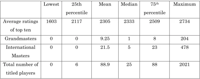
World Chess Federation (FIDE) ratings and titles data were obtained from the FIDE website. Four variables were taken as measures of chess success for each country: average ratings of the top ten active players, number of grandmasters, number of international masters, and total number of titled players. There were a total of 145 countries represented on the FIDE rating list.
Lowest 25th percentile
Mean Median 75th percentile
Maximum
Average ratings of top ten
1603 2117 2305 2333 2509 2734
Grandmasters 0 0 9.25 1 8 204
International Masters
0 0 21.5 5 23 478
Total number of titled players
0 6 88.9 25 88 2021
Table 1. Ratings and titles data
Perhaps the most striking fact is that half of all countries one grandmaster or none; three quarters of them have eight grandmasters or less. Grandmasters are clearly unevenly distributed across the world.
Population data for most countries was obtained from the Central Intelligence Agency’s (CIA) World Factbook. There were three exceptions: England, Scotland and Wales, as the Factbook registered them as one combined entity (the United Kingdom). Population data for these three countries was retrieved from the Office of National Statistics of the United Kingdom.
A country’s income was measured by its Gross Domestic Product per capita, adjusted for costs of living. This was also taken from the CIA World Factbook.
Lowest 25th percentile
Mean Median 75th percentile
Maximum
Population (millions)
0.0210 2.97 42 8.14 29.3 1336
GDP per capita (PPP, i.e. adjusted for cost of living)
$300 $4900 $19 799 $12700 $30200 $145 300
Table 2. Population and income data
Population and GDP per capita are also unevenly distributed. There are a small number of countries with far higher population and GDP than the rest.
3. Methodology
Multiple linear regression with ordinary least squares was used. As the chess success of a country is not easily defined, I created different models with different dependent variables.
4. Results
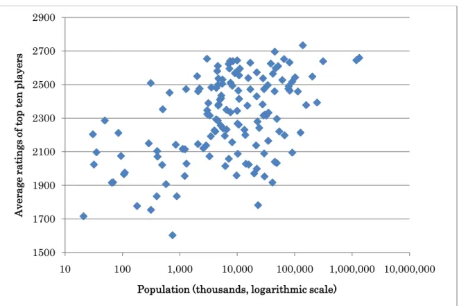
From Figures 1 and 2 that follow, both population and per capita GDP (PPP) seem to have a positive relationship with the average rating of top ten players. However, the relationship between population and average rating seems to be stronger than the relationship between GDP and average rating.
Logarithmic scales are used for both population and GDP. Intuitively, as population grows larger, the benefits of an increasing population decrease gradually; the same goes for GDP. If both Singapore and Russia’s population were increased by 1 million, Russia would benefit much less. Visually, a logarithmic scale also seems to be more appropriate.
Figure 1. Relationship between average rating of top players and population
1500 1700 1900 2100 2300 2500 2700 2900
10 100 1,000 10,000 100,000 1,000,000 10,000,000
A
ve
rag
e
ra
ti
n
gs
o
f t
op
t
en
p
la
ye
rs
Figure 2. Relationship between average rating of top players and GDP per capita (adjusted for cost of living)
Using average rating of top players as the dependent variable
An ordinary least squares model suggests the following:AvgRtg = 300 + 73log(Pop) + 91log(GDP) +
Standard errors: [7.92] [14.3] R2 = 0.407, n = 145
AvgRtg is the average rating of the top ten players, log(Pop) and log(GDP) are the natural logarithms of population and GDP, units being people and US$ respectively. Both coefficients are highly statistically significant. Indeed, for both coefficients, the p-value is less than 10-8. Hence, even though the data show some evidence of
heteroscedasticity, it is highly unlikely that the statistical significance would be affected even if robust standard errors were used. Nor is there any significant multi-collinearity: the correlation coefficient between population and GDP is around –0.10. Finally, the model does not appear to be misspecified: Ramsey’s RESET test gives p-values of more than 0.5 for both the estimated values of Y2 and Y3, and an overall p-value of 0.179.
1500 1700 1900 2100 2300 2500 2700 2900
100 1000 10000 100000 1000000
A
ve
rag
e
ra
ti
n
g
of
t
op
t
en
p
la
ye
rs
The interpretation of the model is simple: Holding all other factors constant, a 1% increase in population of a country increases the average rating of its top ten players by 0.73 points on average. Likewise, a 1% increase in GDP (PPP) would increase average rating by 0.91 points, all else same. However, differences between the income and population of countries only explain 40% of the differences in the strength of top ten players in each country. The other 60% of differences are due to other factors, which may include:
Policies of the national federation (e.g. national training pipeline) Support of the government and sponsors
Other aspects of the chess culture of the country
“Luck”: a country may have a player who is born particularly talented
I would, however, downplay the importance of the last factor, because even if a country has a player that is born particularly talented, his rating is averaged over ten players.
Using total number of titled players as dependent variable
Again, using an ordinary least squares model:
TitledPlayers = –1040 + 40log(Pop) + 53log(GDP) +
Standard errors: [14.6] [8.02] R2 = 0.171, n = 145
Again, the coefficients are significant even at the 0.1% level. Thus, population and GDP are clearly related to the number of titled players. However, in this model, differences in population and GDP between countries only explain 17.1% of the differences in titled players between countries.
According to the model, a 1% increase in a country’s population is expected to increase the number of titled players by 0.4 on average, and holding all other factors constant. Also, an increase in GDP by 1% will increase the number of titled players by 0.53 on average – holding all other factors constant as usual.
Ramsey’s RESET test (with squares and cubes of fitted values) gave a p-value significant the 5% level, indicating the model may have been misspecified. However, adding in non-linear versions log(Pop) and log(GDP) did not seem to make the model any better; in fact, all coefficients became statistically insignificant. Also, theoretically
there was no compelling reason to include squares or cubes or log(Pop) and log(GDP). Thus, the result of the RESET test was ignored.
Because many countries had no grandmasters and/or international masters – in fact, 62 countries had no grandmasters and 41 had no international masters – it would not be appropriate in my view to construct a model with grandmasters or international masters as the dependent variable.
5. Conclusion & Policy Implications
A key conclusion from this paper is that population and GDP, even when combined, do not explain more than half of a country’s chess success. In fact, depending on how one measures chess success, these factors account for 17% to 40% of a country’s chess
success at present. Population and GDP do positively influence a country’s chess success, but being small or poor does not place a country at a large disadvantage. True, it is not so easy to compete with big and rich countries, but a number of the top 20 nations are either small or poor: Armenia, Hungary, Israel, and the Netherlands are four
uncontroversial exceptions.
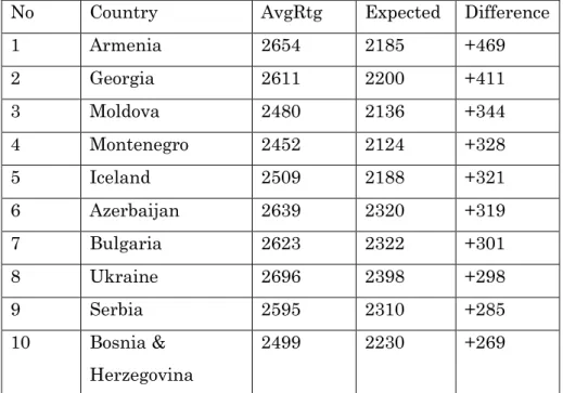
Also, some countries have a much higher rating than would be expected based on their population and GDP. This further supports the notion that other factors are far more important than population or GDP. Their chess culture and chess training pipeline, and policies of their national federations deserve some study.
No Country AvgRtg Expected Difference
1 Armenia 2654 2185 +469
2 Georgia 2611 2200 +411
3 Moldova 2480 2136 +344
4 Montenegro 2452 2124 +328
5 Iceland 2509 2188 +321
6 Azerbaijan 2639 2320 +319
7 Bulgaria 2623 2322 +301
8 Ukraine 2696 2398 +298
9 Serbia 2595 2310 +285
10 Bosnia & Herzegovina
2499 2230 +269
The middle column in table 3 shows the average rating of a country’s top ten players, the next column shows its expected rating based on its population size and GDP, and finally the difference between the two.
National federations should therefore be heartened that they can influence most of their chess success. Some of this influence is more direct and can have effects in the short term, such as the policies of the national federation itself. Other aspects of the chess federation’s influence may be less direct. For example, it may take time to get strong government support and build a good chess culture, but the national federation can do much over the long term.
6. Limitations of this study & suggestions for future research
One key factor in influencing a nation’s chess success is its national training pipeline as well as the policies of the national chess federation. However, it is not immediately obvious how this can be quantified. Future research could quantify these variables as well as measure their impact.
The top ten countries of Table 3 all come from Europe, with Iceland the only country that was not formerly communist. Future research could examine why this is so. Also, the model could be modified with dummy variables across different continents.
Bibliography
Central Intelligence Agency. (May, 2011). World Factbook. Retrieved May, 2011, from https://www.cia.gov/library/publications/the-world-factbook/
FIDE. (May, 2011). FIDE Ratings List. Retrieved May, 2011, from World Chess Federation: http://ratings.fide.com/topfed.phtml
Appendix A: Regression output
Model 1: OLS, using observations 1-145 Dependent variable: AvgRtg
coefficient std. error t-ratio p-value --- const 299.669 212.385 1.411 0.1604 lgPop 73.4049 7.92283 9.265 2.84e-016 *** lgGDP 91.3712 14.3917 6.349 2.74e-09 *** Mean dependent var 2305.717 S.D. dependent var 247.8572 Sum squared resid 5245680 S.E. of regression 192.2015 R-squared 0.407025 Adjusted R-squared 0.398673 F(2, 142) 48.73527 P-value(F) 7.68e-17 Log-likelihood -966.7193 Akaike criterion 1939.439 Schwarz criterion 1948.369 Hannan-Quinn 1943.067
Auxiliary regression for RESET specification test OLS, using observations 1-145
Dependent variable: AvgRtg
coefficient std. error t-ratio p-value --- const 3808.52 12894.0 0.2954 0.7681 logGDP -912.805 2575.15 -0.3545 0.7235 logPop -734.413 2067.92 -0.3551 0.7230 yhat^2 0.00568749 0.0123702 0.4598 0.6464 yhat^3 -9.51209e-07 1.80458e-06 -0.5271 0.5990 Test statistic: F = 1.741256,
with p-value = P(F(2,140) > 1.74126) = 0.179
Model 2: OLS, using observations 1-145 Dependent variable: TotalTitled
coefficient std. error t-ratio p-value --- const -1040.18 214.929 -4.840 3.35e-06 *** logGDP 53.6372 14.5641 3.683 0.0003 *** logPop 40.0022 8.01773 4.989 1.75e-06 *** Mean dependent var 88.85517 S.D. dependent var 212.1872 Sum squared resid 5372097 S.E. of regression 194.5036 R-squared 0.171404 Adjusted R-squared 0.159733 F(2, 142) 14.68708 P-value(F) 1.59e-06 Log-likelihood -968.4457 Akaike criterion 1942.891 Schwarz criterion 1951.822 Hannan-Quinn 1946.520
Appendix B: Complete list of countries
Average rating refers to the average rating of the top ten players as on May 2011. Expected rating would be the expected rating of the top ten players, based solely on the country’s population and GDP.
No Country AvgRtg Expected Difference
1 Armenia 2654 2185 469
2 Georgia 2611 2200 411
3 Moldova 2480 2136 344
4 Montenegro 2452 2124 328
5 Iceland 2509 2188 321
6 Azerbaijan 2639 2320 319
7 Bulgaria 2623 2322 301
8 Ukraine 2696 2398 298
9 Serbia 2595 2310 285
10 Bosnia & Herzegovina 2499 2230 269
11 Croatia 2581 2317 264
12 Cuba 2595 2331 264
13 Hungary 2644 2383 261
14 Former YUG Rep of
Macedonia 2460 2203 257
15 Mongolia 2390 2138 252
16 Slovenia 2550 2302 248
17 Uzbekistan 2537 2293 244
18 Faroe Islands 2286 2043 243
19 Estonia 2473 2232 241
20 Israel 2640 2402 238
21 Latvia 2476 2246 230
22 Belarus 2574 2348 226
23 Monaco 2204 2000 204
24 Lithuania 2483 2290 193
25 Romania 2573 2395 178
26 Tajikistan 2335 2157 178
27 Russia 2734 2560 174
28 Czech Republic 2581 2412 169
29 Turkmenistan 2410 2246 164
30 Kazakhstan 2539 2379 160
31 Slovakia 2505 2353 152
32 Philippines 2543 2399 144
33 Poland 2625 2481 144
34 Netherlands 2630 2490 140
35 Albania 2347 2208 139
36 Vietnam 2517 2379 138
37 Denmark 2530 2400 130
No Country AvgRtg Expected Difference
39 Greece 2555 2431 124
40 Paraguay 2350 2227 123
41 Norway 2536 2431 105
42 Argentina 2565 2464 101
43 Andorra 2212 2115 97
44 Burundi 2088 2005 83
45 France 2652 2572 80
46 Peru 2473 2395 78
47 Switzerland 2511 2438 73
48 Nicaragua 2239 2170 69
49 Chile 2472 2403 69
50 India 2645 2576 69
51 Spain 2598 2536 62
52 Luxembourg 2353 2297 56
53 Austria 2493 2437 56
54 England 2610 2559 51
55 Finland 2435 2392 43
56 Ecuador 2375 2334 41
57 Uruguay 2316 2276 40
58 Germany 2632 2595 37
59 Dominican Republic 2344 2310 34
60 Egypt 2464 2435 29
61 Scotland 2419 2391 28
62 Colombia 2460 2432 28
63 Barbados 2150 2134 16
64 Belgium 2464 2449 15
65 Bangladesh 2378 2365 13
66 Bolivia 2268 2258 10
67 Palestine 2121 2111 10
68 Portugal 2415 2406 9
69 Iraq 2321 2313 8
70 Costa Rica 2286 2279 7
71 San Marino 2024 2020 4
72 China 2659 2656 3
73 Jordan 2233 2235 -2
74 Turkey 2490 2495 -5
75 Brazil 2548 2553 -5
76 Iran 2475 2485 -10
77 Ireland 2375 2389 -14
78 Yemen 2242 2266 -24
79 Myanmar 2221 2246 -25
80 Wales 2324 2351 -27
No Country AvgRtg Expected Difference
82 Morocco 2315 2344 -29
83 Italy 2527 2560 -33
84 Syria 2280 2317 -37
85 Venezuela 2382 2420 -38
86 Canada 2497 2540 -43
87 Singapore 2382 2429 -47
88 US Virgin Islands 1976 2027 -51
89 Liechtenstein 2097 2152 -55
90 Algeria 2333 2389 -56
91 Uganda 2165 2222 -57
92 Tunisia 2261 2324 -63
93 New Zealand 2293 2356 -63
94 El Salvador 2195 2259 -64
95 Jersey 2075 2141 -66
96 Lebanon 2221 2292 -71
97 Honduras 2157 2230 -73
98 Mexico 2459 2532 -73
99 Puerto Rico 2227 2302 -75
100 Panama 2192 2268 -76
101 Jamaica 2138 2217 -79
102 United States of
America 2639 2719 -80
103 Surinam 2022 2102 -80
104 Australia 2430 2511 -81
105 Botswana 2146 2233 -87
106 Guatemala 2200 2288 -88
107 Indonesia 2393 2482 -89
108 Sao Tome and Principe 1777 1873 -96
109 Aruba 1966 2062 -96
110 Angola 2231 2333 -102
111 Malta 2071 2180 -109
112 Malawi 2024 2138 -114
113 Cyprus 2117 2231 -114
114 Nepal 2090 2210 -120
115 Malaysia 2316 2437 -121
116 Trinidad & Tobago 2115 2243 -128
117 Mali 2028 2156 -128
118 Brunei Darussalam 2104 2236 -132
119 Palau 1716 1852 -136
120 United Arab Emirates 2257 2403 -146 121 Papua New Guinea 2015 2162 -147
122 South Africa 2296 2447 -151
123 Haiti 1959 2129 -170
No Country AvgRtg Expected Difference
125 Mauritius 2029 2202 -173
126 Guernsey 1916 2091 -175
127 Sri Lanka 2138 2315 -177
128 Ethiopia 2095 2276 -181
129 Maldives 1835 2016 -181
130 Bermuda 1918 2136 -218
131 Fiji 1835 2069 -234
132 Afghanistan 1953 2194 -241
133 Qatar 2142 2388 -246
134 Thailand 2198 2451 -253
135 Sudan 2040 2296 -256
136 Cameroon 1971 2240 -269
137 Macau 1907 2224 -317
138 Bahrain 1956 2297 -341
139 Kenya 1917 2261 -344
140 Hong Kong 2058 2438 -380
141 Japan 2214 2623 -409
142 Bahamas 1754 2166 -412
143 Guyana 1603 2098 -495
144 South Korea 2033 2542 -509