Solving the
k
-center Problem
Ef
fi
ciently with a Dominating Set
Algorithm
Jurij Miheli
c and Borut Robi
ˇ
c
ˇ
Faculty of Computer and Information Science, University of Ljubljana, Slovenia
We present a polynomial time heuristic algorithm for the minimum dominating set problem. The algorithm can readily be used for solving the minimumα-all-neighbor dominating set problem and the minimum set cover problem. We apply the algorithm in heuristic solving the minimumk-center problem in polynomial time. Using a standard set of 40 test problems we experimentally show that ourk-center algorithm performs much better than other well-known heuristics and is competitive with the best known (non-polynomial time) algorithms for solving thek-center problem in terms of average quality and deviation of the results as well as the execution time.
Keywords: combinatorial problems, graph algorithms, performance evaluation, facility location,k-center, domi-nating set.
1. Introduction
Problems of finding the best location of fa-cilities in networks or graphs abound in prac-tical situations, such as determining locations for fabrication, assembly plants, warehouses, airline crew scheduling or tool selection 3, 15]. One of the well known facility location prob-lems is thevertex k-centerproblem, where given
ncities and distances between all pairs of cities, the aim is to choosekcities(calledcenters)so that the largest distance of any city to its nearest center is minimal. Formally, the vertexk-center is defined as follows.
Definition 1. (Vertexk-center problem) Let G = (V E) be a complete undirected graph
with edge costs satisfying the triangle inequal-ity, and k be a positive integer not greater than
jVj. For any set S V and vertex v 2V, define
d(v S)to be the length of a shortest edge from
v to any vertex in S. The problem is tofind such a set S V, wherejSj k, which minimizes maxv2Vd
(v S).
The vertex k-center problem is NP-hard 6], so exact polynomial algorithm is unlikely to exist. A popular way to solve thek-center prob-lem consists of solving a series ofminimum set cover problems 3, 5, 10, 11], where one must locate a minimum number of centers such that every vertex in the graph can be reached (i.e.
covered)within a givencoverage distance. At each step, a threshold for the coverage distance is chosen and the corresponding minimum set cover problem is solved. If the solution contains at most k centers the threshold is decreased, otherwise it is increased. Each of the mini-mum set cover problems is usually solved using integer linear programming. Minieka 11]was among the first to use this approach. Later, how-ever, more elaborate versions were described, such as Daskin 3], Ellumni et al. 5]as well as Ilhan et al. 10], which applied more efficient integer programming definition of the problem. Another approach was given by Daskin 4]who efficiently used maximum cover problem in-stead of the minimum set cover problem. A set of completely different approaches to solve the
k-center problem was given by Mladenovi´c et al. 12], where thetabu search,variable
in the sense that nor-approximation algorithm exists withr <2, unless P= NP 8]. (Notice, that when the triangular inequality does not hold no constant approximation ratio algorithm ex-ists, unless P=NP.)
In this paper we solve thek-center problem as a series of aminimum dominating setproblems 8, 9, 13](as opposed to the series of minimum set cover or maximum cover problems). Given a graph, the minimum dominating set problem asks for a minimum size subsetD of vertices, such that every other vertex is adjacent to at least one of vertices inD. The main reason that we use this approach is that the minimum dominat-ing set problem can be identified as one of the main subproblems when solving the k-center problem. Unfortunately, the minimum domi-nating set problem is stillNP-hard 6], as are the minimum set cover problem and maximum cover problem.
In the following section we describe a heuristic algorithm for the dominating set problem. In Section 3 we show how this algorithm can be applied to solve thek-center problem. Section 4 briefly gives some other possible applications of the dominating set algorithm. Finally, in Section 5 we present experimental results that we obtained by comparing our algorithm with several other well-known algorithms for thek -center problem. For comparison, we used a standard test library and results that were pre-sented in recent literature.
2. A Dominating Set Algorithm
In this section we present a heuristic algorithm for solving the minimum dominating set prob-lem. This problem is formally defined as fol-lows.
Definition 2. (Dominating set) Let G=(V E)
be a graph. A set D V, such that every vertex v 2V ;D is adjacent to at least one vertex in
D, is called dominating set of G.
Definition 3. (Minimum dominating set pro-blem)Given a graph,find a dominating set with minimum cardinality.
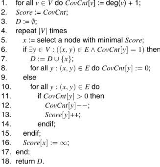
Let us first briefly present the main ideas of the heuristic algorithm for the minimum domi-nating set problem(see algorithm in Figure 1).
Input:graphG=(V E) Output:dominating setD
Algorithm:
1. for allv2VdoCovCnt[v] := deg(v) + 1; 2. Score:=CovCnt;
3. D:=;
4. repeatjVjtimes
5. x:= select a node with minimalScore; 6. if9y2V:((x y)2E^CovCnty]=1)then 7. D:=Dfxg;
8. for ally:(x y)2EdoCovCnty]:=0; 9. else
10. for ally:(x y)2Edo 11. ifCovCnty]>0then 12. CovCnty] ;;; 13. Scorey]++; 14. endif;
15. endif;
16. Scorex]:=1; 17. end;
18. returnD.
Fig. 1.The dominating set heuristic algorithm.
Initially, the dominating set is empty, D := . During the algorithm the setDgrows according to the ‘lazy’ principle, i.e. enlargeDas late as possible. For each vertex v 2 V we keep the countCovCnt v], which is the number of times the vertex is covered by the remaining vertices and is initialized to deg(v)+1, where deg(v) denotes the degree ofv.
We also estimate the ‘importance’ ofvby apply-ing a specialscoringstrategy to rank the vertices as potential centers. Then, at each step, a vertex
x with minimal score ischecked, i.e. if there is an adjacent vertex having cover count 1, thenx
is added toD; otherwisexis used to decrement cover counts and increment scores of its not yet covered adjacent vertices.
Detailed description. Lines 1–3 are the ini-tialization part of the algorithm. In addition to setting D to empty set, they also initialize two arrays. The first array is CovCnt, where
CovCnt v] is the number of vertices currently covered by(i.e. adjacent to)v. We assume that
vis adjacent to itself. The second array, called
reflect the rule of thumb that vertices with low degrees should be checked first.
Lines 4–17 are the main loop of the algorithm. At each execution of the loop a vertex x with minimal score is selected (line 5). Next, it is checked if x has a neighbor with cover count equal to 1 (line 6). If so, the vertex x is the only possible remaining vertex in the graph that can cover such a neighbor. Hence, x must be added to the current dominating setD. Cover counts of all neighbors ofx are set to 0 to des-ignate them as covered (lines 7,8). If x has no neighbor with cover count 1, it is used to improve the current heuristic scoring of those among its neighbors that are still not covered
(lines 10–14). To do this, cover counts of x’s neighbors are decremented(because x doesn’t cover them anymore)while their scores are in-cremented (they worth more). At the end of the loop-body the vertex x is designated to be checked by settingScore x]to infinity.
Correctness. Clearly, the algorithm termi-nates afterjVjexecutions of the loop body. The algorithm returns a dominating set of the input graph. To see this, consider separately isolated and non-isolated vertices of a graph. First, all the possible isolated vertices(Score x]= 1)of the graph are checked and added(CovCnt x]= 1) to the dominating set D. After all isolated vertices have been checked, the algorithm con-tinues on non-isolated vertices, i.e. vertices with initial cover count and score greater than 1. Now consider a non-isolated vertexy. The vertex will be covered either because one of its neighbors, say x, has been added to D(due to some x’s neighbor z 6= y with cover count 1) or becausey’s cover count has reached 1 after
deg(y)decrements(because at each step a dif-ferent vertex x 2 V is checked). Thus, every non-isolated vertex will be covered, too. Con-sequently, all the vertices of the input graph will be covered, so the algorithm in Figure 1 finds a dominating set.
Complexity. Let us write n = jVj. The ini-tialization (lines 1–3) takes O(n
2
) time. The body of the main loop is executed ntimes. At each execution the minimal score vertex can be found inO(n) time. The condition(line 6)as well as inner loops(lines 8 and 10–14)can all be evaluated inO(n)time. Thus, the algorithm terminates inO(n
3
)time. However, if vertices are always processed in the same order ( de-termined by a listL), the time complexity can easily be reduced toO(n
2
)by using
backtrack-ing. More precisely, suppose that theelse part (lines 10–14)is to be executed. While process-ing the vertices (line 10) one can also check if the condition (line 6) is still false. If the condition has become true, loop is broken, the current vertex is remembered as the backtrack vertexand backtracking procedure is started. In this procedurexis added toDandx’s neighbors are processed, i.e. their cover counts are set to 0 and each neighbor’s score is decremented if the neighbor is located before the backtrack vertex inL. Thus, backtracking gives two sepa-rate innerforloops each with time complexity
O(n).
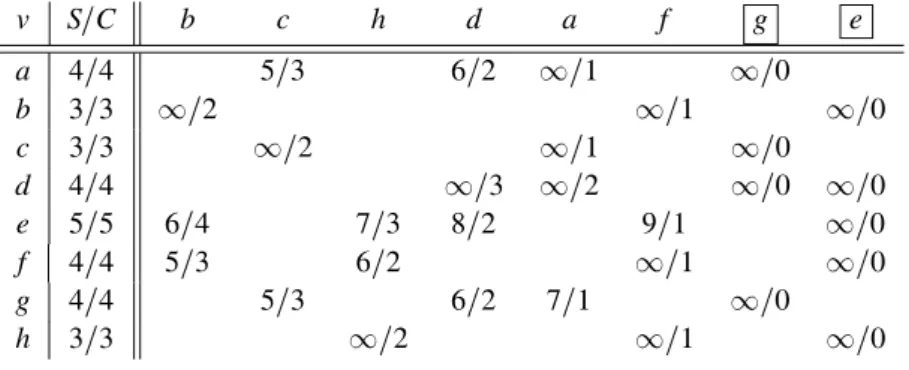
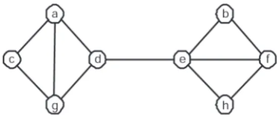
Example. Let us demonstrate a simple exam-ple on how the dominating set algorithm from Figure 1 works on a network shown in Figure 2. There are 8 vertices in this network, thus the algorithm will execute in 8 steps. Execution of the algorithm is shown in Table 1. The first
v S=C b c h d a f g e
a 4/4 5/3 6/2 1/1 1/0
b 3/3 1/2 1/1 1/0
c 3/3 1/2 1/1 1/0
d 4/4 1/3 1/2 1/0 1/0
e 5/5 6/4 7/3 8/2 9/1 1/0
f 4/4 5/3 6/2 1/1 1/0
g 4/4 5/3 6/2 7/1 1/0
h 3/3 1/2 1/1 1/0
Fig. 2.Example network for dominating set problem.
column lists all of the network vertices. The second columnS=Cshows the scores and cover counts for each vertex after initialization part of the algorithm. Columns 3–10 give values of score and cover count after each step(only val-ues of processed vertices are shown). The first row contains the vertex that is being processed. For example, in the third column the first step of the algorithm is shown where vertexbis pro-cessed (has minimal score). Vertex b is not added to D because all of its neighbors have cover count greater than 1. Thus, score is in-cremented and cover count is dein-cremented, for all b’s neighbors. Score of b is set to 1. In the ninth column of the table vertex g is pro-cessed and it must be added to D because at least one ofg’s neighbors has cover count equal to 1(vertices a c and g). All cover counts of
g’s neighbors are set to 0 to designate them as covered.
3. Application to thek-center Problem
The algorithm for solving the k-center prob-lem uses described dominating set algorithm and parametric pruning, an algorithmic tech-nique presented in 9, 14, 17], The algorithm is calledScrand is formally described in Figure 3. Initially, edge costs are sorted in nondecreasing
order. For each edge cost tthe graph is pruned by removing edges with cost greater thantand the minimum dominating setC is found in the pruned graph (BottleneckGraph). If the size ofCis less than or equal tok, thenCis also the optimal solution of the k-center problem. As we already mentioned, the minimum dominat-ing set problem isNP-hard. To obtain efficient algorithm for the k-center problem we applied our algorithm in Figure 1 and the parametric pruning technique from Figure 3.
Complexity. The first phase of the Scr algo-rithm, which is sorting of the edge costs, takes
O(mlogm)=O(n 2logn
)time. The main loop
(lines 2–6)takes O(m) = O(n 2
) time. Nodes
u and v are adjacent in the pruned graph if the distance d(u v) ci, which can directly be used in DominatingSet procedure. Thus, the algorithm Scr has polynomial time complex-ity O(mn
3
) = O(n 5
). Notice that by using binary search instead of iterative search (line 2), and by using backtracking in the Dominat-ingSet procedure, the time complexity of the
k-center algorithm can easily be reduced to
O(n 2logm
)=O(n 2logn
).
4. Other Applications
The algorithm in Figure 1 can easily be extended to solve another version of the dominating set, calledminimumα-all-neighbor dominating set
problem where the aim is to cover every ver-tex(even centers)with at leastα 1 vertices. To do this, one simply changes the condition in line 6 of the algorithm. In particular, in-stead of checking ifCovCnt y] =1, the equal-ity CovCnt y] = α must be checked. Notice, however, that feasible solution of such a prob-lem may not exist, so one should check at the
Input:complete graphG=(V E)with edge costs Output:set of centersC
Algorithm:
1. sort edge costs into nondecreasing listc1,c2,:::,cmwherem=jEj; 2. for allci:=c1tocmdo
3. Gi:= BottleneckGraph(G ci); 4. C:= DominatingSet(Gi); 5. ifjCjkthen returnC; 6. end.
beginning(after line 1)if all cover counts are
α. Further, if applying this algorithm to the
k-center algorithm in Figure 3, we obtain the al-gorithm for minimum α-all-neighbor k-center
problem.
Additionally, one can apply the idea of vertex scores and cover counts to solve the well-known
minimum set coverproblem where, given a fam-ilyF = fS1 S2 ::: SNg of subsets of a finite setX=fx1 x2 ::: xng, such thatX =S
2FS, the aim is to find a minimum cardinality subset
C F such that every element of X belongs to at least one set inC. To find a minimum set cover the algorithm in Figure 1 is changed to track cover count for each elementx 2 X and score for every set S 2 F. Variable x in the algorithm now represents a set with minimal score, the variabley represents elements of X, while the relation(x y) 2 E stands fory 2 x. Line 13 must also be changed to increment the score of all sets containingy.
5. Experimental Results
In this section we briefly describe several im-plemented and tested algorithms for thek-center problem. After describing the testing environ-ment we discuss experienviron-mental results obtained on a set of 40 standard test problems 1].
Implemented algorithms. A very simple heu-ristic to solve thek-center problem is thepure greedy method, where centers are located con-secutively so that the objective function is each time reduced as much as possible. We tested
three approaches to locate the first center: (1) random, (2) take the solution of the 1-center algorithm, or (3) start from the vertex that of-fers the best solution (here n runs have to be made). These approaches are called random (GrR),1-center (Gr1), and plus(Gr+) version, respectively.
Another greedy heuristic for thek-center prob-lem was described by Gonzalez 7] and Dyer and Frieze 2]. They were able to prove the approximation factor of 2. At each step of Gon-zalez algorithm the vertex that is the farthest from the current set of centers is added to this set. We implemented and tested the random
(GonR), 1-center(Gon1)and plus(Gon+)version of Gonzalez algorithm.
Shmoys 16]briefly described a 2-approximation algorithm for the decision version of k-center problem. Here, radiusris given and the aim is to decide if there arekvertices so that the cov-erage distance from these vertices is at mostr. The algorithm repeatedly chooses one of the re-maining verticesv, adds it to the partial solution and deletes all the vertices whose distance tovis at most 2r. At the end, if the size of the solution exceeds k, the algorithm outputs “no”, other-wise “yes”. Based on this we implemented two optimization versions of this algorithm, where either random(ShR)vertex or vertex with max-imum degree(ShD)is chosen at each step. Hochbaum and Shmoys introduced the algo-rithmic technique calledparametric pruningfor solving the k-center problem 9, 17]. Initially, edge costs are sorted in nondecreasing order and for each edge costta maximal independent set in the square of the pruned graph is found.
Approximation factor
Algorithm average deviation Description
GrR 1.697 0.559 Pure greedy first random Gr1 1.675 0.570 Pure greedy first 1-center Gr+ 1.512 0.550 Pure greedy plus
GonR 1.495 0.130 Gonzalez first random HS 1.462 0.177 Hochbaum-Shmoys ShR 1.432 0.112 Shmoys random Gon1 1.398 0.128 Gonzalez first 1-center
ShD 1.343 0.105 Shmoys degree Gon+ 1.317 0.139 Gonzalez plus
Scr 1.058 0.043 Scoring heuristic
If the set contains no more than k vertices, it is returned as the solution of thek-center prob-lem; otherwise, the thresholdtis increased. The authors have proved that this algorithm(HS) re-turns 2-approximate solutions. The mentioned algorithms are listed in Table 2. Notice that we also included our algorithm(Scr).
Testing environment. For testing the de-scribed algorithms we used the standard OR-Library, which contains 40 test graphs. These graphs contain from 100 to 900 vertices whilek
ranges from 5 to 90. Originally, the library was designed for testingk-median problems 1], but it has become also a standard testing tool for the
k-center problem because the optimal solutions are known. They had been obtained mostly with integer programming approaches 4, 5, 10], tabu search or variable neighbourhood search 12].
(The preprocessing runs the all shortest paths algorithm with time complexityO(n
3 )).
We implemented all the algorithms from Table 2 in Borland Delphi 7.0 and tested on a com-puter with Intel processor running at 1700 MHz with 512MB of system memory.
Experimental results. Although our primary aim was to compare the quality of the solutions, let us mention that Gonzalez’s algorithms were the fastest(running below 1 second). The pure greedy methods were quite fast(about 1.5 sec-onds on average), but their execution time was very variable and dependent on the parameterk. (Recall, thatplusvariants run much slower due to the algorithm which tries all vertices for the first center.) The average time ofHSwas about
Running time Algorithm average deviation
GonR 0.006 0.01 Gon1 0.01 0.012
ShR 0.204 0.142 ShD 0.211 0.147 GrR 1.526 2.37 Gr1 1.565 2.37 Gon+ 2.407 3.85
Scr 11.92 10.77
HS 37.85 45
Gr+ 823 1456
Table 3.Running times of the algorithms.
38 seconds. Shmoys’ variants were also quite fast(below 1 second)and theScrrunning time was 12 seconds on average. Average running times of the algorithms are summarized in the following table.
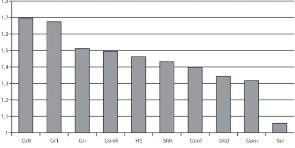
Recall that approximation factor is defined to be the ratio between approximate and optimal solution. Average approximation factors for the algorithms compared are given in Table 3 above. The entries are sorted according to the average quality of the approximate solutions.
Having the smallest average approximation fac-tor, our Scr algorithm performs much better than any other heuristic approach. In addition, this algorithm exhibits the smallest deviation of the approximation factor. Figure 4 also shows that there is a considerable quality leap between
Scr algorithm and Gon+, which is the second best of these algorithms.
# n k Opt GrR Gr1 GrP Gon Gon1 Gon+ HS ShR ShD Scr 1 100 5 127 143 133 133 186 162 155 184 188 171 133 2 100 10 98 117 117 110 131 124 117 160 128 135 109 3 100 10 93 126 116 106 154 133 124 160 140 120 99 4 100 20 74 127 127 92 114 99 92 124 109 84 83
5 100 33 48 87 87 78 71 64 62 77 62 59 48
6 200 5 84 98 94 89 138 99 98 126 138 106 90
7 200 10 64 78 79 77 96 87 85 90 88 90 70
8 200 20 55 72 72 72 82 72 71 84 74 68 60
9 200 40 37 73 73 63 57 51 49 62 50 52 38
10 200 67 20 44 44 38 31 29 29 32 28 28 20
11 300 5 59 68 67 61 73 68 68 82 73 74 60
12 300 10 51 62 72 56 71 70 66 78 74 70 53
13 300 30 35 64 64 52 59 51 49 60 54 52 38
14 300 60 26 60 60 46 40 36 36 44 36 34 27
15 300 100 18 42 42 40 25 25 23 30 22 20 18
16 400 5 47 52 51 47 84 55 52 64 83 58 48
17 400 10 39 50 50 43 56 51 48 56 56 52 41
18 400 40 28 50 50 42 44 41 39 46 40 38 31
19 400 80 18 40 40 31 28 28 27 30 26 24 20
20 400 133 13 32 32 32 19 19 17 22 18 16 14
21 500 5 40 48 48 42 53 51 45 52 53 45 40
22 500 10 38 48 49 43 56 54 47 54 54 48 41
23 500 50 22 41 41 35 34 33 32 36 32 30 24
24 500 100 15 35 35 32 23 23 21 24 22 20 17
25 500 167 11 27 27 27 15 15 15 18 16 14 11
26 600 5 38 44 43 39 50 47 43 52 50 52 41
27 600 10 32 37 39 35 43 42 55 42 44 44 33
28 600 60 18 33 33 27 28 28 25 28 28 28 20
29 600 120 13 34 36 34 19 19 18 22 18 18 13
30 600 200 9 29 29 29 14 14 13 16 12 12 10
31 700 5 30 35 34 31 42 38 36 40 42 44 30
32 700 10 29 35 35 32 45 43 37 40 44 40 31
33 700 70 15 32 26 24 26 25 23 26 24 22 17
34 700 140 11 30 30 27 17 17 16 18 16 16 11
35 800 5 30 37 32 31 38 37 34 40 38 38 32
36 800 10 27 34 34 30 41 41 34 38 42 38 28
37 800 80 15 26 26 26 25 24 23 24 22 22 16
38 900 5 29 42 35 31 36 38 31 38 40 38 29
39 900 10 23 27 28 25 35 35 28 32 36 34 24
40 900 90 13 25 22 22 21 20 19 22 20 20 14
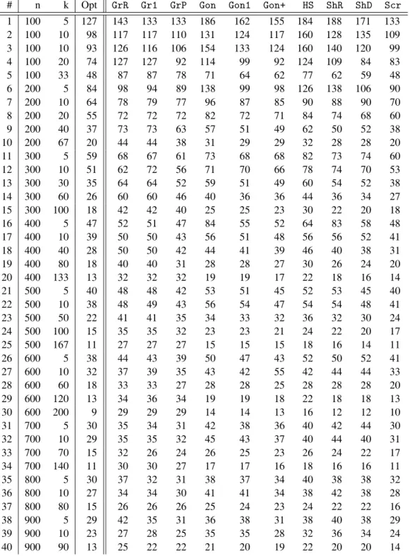
Table 4.Experimental results: # is the graph number;nrepresents the number of vertices;kis the number of centers; Opt is the optimal result; other columns contain results obtained with corresponding algorithms.
The results for particular algorithms and prob-lems are given in Table 4. Pure greedy algo-rithms were the worst, while only slightly better results were obtained with the plus version. By examining Table 4 we found out that the quality of the pure greedy method strongly depends on the parameterkand improves for low values of
k. Gonzalez algorithms are very fast. The best variant of the Gonzalez algorithm is the plus variant, yet it still returns results that are about 32% above the optimal. The algorithms HS,
The algorithmScrachieved better results than any other of the implemented algorithms and is also quite competitive with integer program-ming and metaheuristic approaches. In particu-lar, the solutions ofScrheuristic are on average only 6% above the optimal.
6. Conclusions
In this paper we have presented a polynomial time heuristic algorithm for the minimum dom-inating set problem, which uses the so-called scoring technique. We applied this algorithm to efficiently solve thek-center problem. Then we experimentally evaluated our algorithm and several other well-known heuristic algorithms for thek-center problem. To do this, we used the standard set of 40 test problems. The ex-perimental results show that our algorithm is comparable with the best known algorithms for solving thek-center problem 4, 5, 10]. These algorithms were able to solve quickly enough each of the forty test problems to optimality. Since they rely on the integer programming, it would be interesting to see how they per-form on larger test instances. We have also found that, surprisingly, the performance of the well-known 2-approximation algorithm HS by Hochbaum and Shmoys 9] was quite unsatis-factory, as was noticed also by Mladenovi´c 12]. The same is true for all the tested approxima-tion algorithms. These are all three versions of Gonzalez algorithm(Gon,Gon1,Gon+)and both Shmoys algorithms(ShR,ShD). The pure greedy approach is the worst among all and if, for any reason, it is used, we suggest using it only for small values ofk.
Finally, in the paper we have shown that our heuristic algorithm for solving the minimum dominating set problem can easily be adapted to solve several other important combinatorial op-timization problems. Among these are (1)the minimumα-all-neighbor dominating set prob-lem, (2) the minimum set cover problem, and
(3)the α-all-neighbor k-center algorithm. An interesting future research would be to experi-mentally evaluate, for each of these problems, the corresponding adapted algorithm and com-pare it with the currently best algorithms.
References
1] J.E. BEASLEY, A note on solving large p-median problems, European J. Oper. Res., 21:270–273, 1985.
2] M.E. DYER ANDA.M. FRIEZE, A simple heuristic for thep-centre problem,Operations Research Letters, 3:6:285–288, 1985.
3] M.S. DASKIN, Network and Discrete Location:
Models Algorithms and Applications, Wiley, New York, 1995.
4] M.S. DASKIN, A new approach to solving the ver-tex p-center problem to optimality: Algorithm and computational results,Communications of the Op-erations Research Society of Japan, 45:9:428–436, 2000.
5] S. ELLOUMI, M. LABBE,ANDY. POCHET, New for-mulation and resolution method for the p-center problem, 2001. http://www.optimization;
online.org/DB HTML/2001/10/394.html.
6] M.R. GAREY ANDD.S. JOHNSON, Computers and
Intractability: A Guide to the Theory of NP-Completeness, W.H. Freeman and Co., San Fran-cisco, 1979.
7] T. GONZALEZ, Clustering to minimize the maxi-mum intercluster distance, Theoretical Computer Science., 38:293–306, 1985.
8] D.S. HOCHBAUM, ed., Approximation Algorithms
for NP-hard Problems, PWS publishing company, Boston, 1995.
9] D.S. HOCHBAUM ANDD.B. SHMOYS, A best possi-ble heuristic for the k-center propossi-blem,Mathematics of Operations Research, 10:180–184, 1985.
10] T. ILHAN AND M.C. PINAR, An efficient exact algorithm for the vertex p-center problem, 2001. http://www.optimization-online.org/
DB HTML/2001/09/376.html.
11] E. MINIEKA, The m-center problem, SIAM Rev., 12:138–139, 1970.
12] N. MLADENOVIC´, M. LABBE,ANDP. HANSEN, Solv-ing the p-center problem with tabu search and vari-able neighborhood search,Networks42(1):48–64, 2003.
13] J. MIHELIC ANDˇ B. ROBICˇ, Approximation algo-rithms fork-center problem: an experimental eval-uation,Proc. OR 2002, Klagenfurt, Austria, 2002.
14] J. PLESNIK, A Heuristic for thep-Center Problem in Graphs,Discrete Applied Mathematics17:263–268, 1987.
16] D.B. SHMOYS, Computing near-optimal solutions to combinatorial optimization problems, Technical re-port, Ithaca, NY 14853, 1995.http://citeseer.
nj.nec.com/shmoys95computing.html.
17] V. VAZIRANI, Aproximation Algorithms, Springer, 2001.
Received:September, 2005
Accepted:March, 2005
Contact address:
Jurij Mihelicˇ
Faculty of Computer and Information Science University of Ljubljana Trzaˇ ˇska 25, 10000 Ljubljana, Slovenia e-mail:[email protected]
Web:http://lalg.fri.uni-lj.si/ jure
JURIJMIHELIˇCreceived the BSc (2001)and MSc(2004)degrees in
computer science from the University of Ljubljana, Slovenia. He is presently working towards his PhD at the Faculty of Computer and In-formation Science, University of Ljubljana. His fields of interests are facility location, combinatorial optimization and approximation algo-rithms.
BORUTROBIˇCis Professor of computer science at the Faculty of Com-puter and Information Science, University of Ljubljana, Slovenia. Fol-lowing completion of his B.Sc.(1984), M.Sc.(1987), and D.Sc.(1993)