Probability distribution relationships

PROBABILITY DISTRIBUTION RELATIONSHIPS

Y.H. Abdelkader, Z.A. Al-Marzouq

1.INTRODUCTION

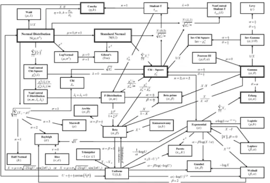
In spite of the variety of the probability distributions, many of them are related to each other by different kinds of relationship. Deriving the probability distribu-tion from other probability distribudistribu-tions are useful in different situadistribu-tions, for ex-ample, parameter estimations, simulation, and finding the probability of a certain distribution depends on a table of another distribution. The relationships among the probability distributions could be one of the two classifications: the transfor-mations and limiting distributions. In the transfortransfor-mations, there are three most popular techniques for finding a probability distribution from another one. These three techniques are:

1 - The cumulative distribution function technique 2 - The transformation technique

3 - The moment generating function technique. The main idea of these techniques works as follows:

For given functions g X Xi( 1, 2, ...,Xn), for i 1, 2, ...,k where the joint

dis-tribution of random variables (r.v.’s) X X1, 2, ...,Xn is given, we define the

func-tions

1 2

( , , ..., ), 1, 2, ...,

i i n

Y g X X X i k (1)

The joint distribution of Y Y1, 2, ...,Yn can be determined by one of the

suit-able method sated above. In particular, for k 1, we seek the distribution of ( )

Y g X (2)

For some function ( )g X and a given r.v. X.

The equation (1) may be linear or non-linear equation. In the case of linearity, it could be taken the form

1 n

i i i

Many distributions, for this linear transformation, give the same distributions for different values for ai such as: normal, gamma, chi-square and Cauchy for

continuous distributions and Poisson, binomial, negative binomial for discrete distributions as indicated in the Figures by double rectangles. On the other hand, when 1ai , the equation (3) gives another distribution, for example, the sum of

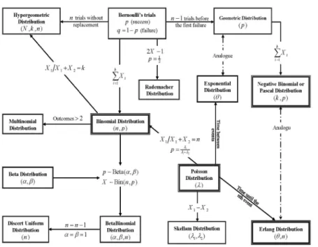
the exponential r.v.’s gives the Erlang distribution and the sum of geometric r.v.’s gives negative- binomial distribution as well as the sum of Bernoulli r.v.’s gives the binomial distribution. Moreover, the difference between two r.v.’s give an-other distribution, for example, the difference between the exponential r.v.’s gives Laplace distribution and the difference between Poisson r.v.’s gives Skellam dis-tribution, see Figures 1 and 2.

In the case of non-linearity of equation(1), the derived distribution may give the same distribution, for example, the product of log-normal and the Beta distri-butions give the same distribution with different parameters; see, for example, (Crow and Shimizu, 1988), (Kotlarski, 1962), and (Krysicki, 1999). On the other hand, equation (1) may be give different distribution as indicated in the Figures.

The other classification is the asymptotic or approximating distributions. The asymptotic theory or limiting distribution provides in some cases exact but in most cases approximate distributions. These approximations of one distribution by another one exist. For example, for large n and small p the binomial distribu-tion can be approximated by the Poisson distribudistribu-tion. Other approximadistribu-tions can be given by the central limit theorem. For example, for large n and constantp, the central limit theorem gives a normal approximation of the binomial distribu-tion. In the first case, the binomial distribution is discrete and the approximating Poisson distribution is also discrete. While, in the second case, the binomial dis-tribution is discrete and the approximating normal disdis-tribution is continuous. In most cases, the normal or standard normal plays a very predominant role in other distributions.

The most important use of the relationships between the probability distribu-tions is the simulation technique. Many of the methods in computational statistics require the ability to generate random variables from known probability distribu-tions. The most popular method is the inverse transformation technique which deals with the cumulative distribution function, ( )F x , of the distribution to be simulated. By setting

( )

F x U

Where ( )F x and U are defined over the interval (0,1) and U is a r.v. follows the uniform distribution. Then, x is uniquely determine by the relation

1_{( )}

x F U ₍₄₎

so complicated as to be impractical. When this is the case, another distribution with a simple closed form can be used and derived from another or other distri-butions. For example, to generate an Erlang deviate we only need the sum m ex-ponential deviates each with expected value 1 m. Therefore, the Erlang variate

x is expressed as

1 1

1 _ln

m m

i i

i i

x y U

T

¦

¦

Where yi is an exponential deviate with parameter T, generated by the

in-verse transform technique and Ui is a random number from the uniform

distri-bution. Therefore, a complicated situation as in simulation models can be re-placed by a comparatively simple closed form distribution or asymptotic model if the basic conditions of the actual situation are compatible with the assumptions of the model.

The relationships among the probability distributions have been represented by (Leemis, 1986), (Taha, 2003) and (Rider, 2004) in limited attempts. The first and second authors have presented a diagram to show the relationships among probability distributions. The diagrams have twenty eight and nineteen distribu-tions including: continuous, discrete and limiting distribudistribu-tions, respectively. The Rider’s diagram divided into four categories: discrete, continuous, semi-bounded, and unbounded distributions. The diagram includes only twenty distributions. This paper presents four diagrams. The first one shows the relationships among the continuous distributions. The second diagram presents the discrete distribu-tions as well as the analogue continuous distribudistribu-tions. The third diagram is con-cerned to the limiting distributions in both cases: continuous and discrete. The Balakrishnan skew-normal density and its relationships with other distributions are shown in the fourth diagram. It should be mentioned that the first diagram and the fourth one are connected. Because the fourth diagram depends on some continuous distributions such as: standard normal, chi-square, the standard Cauchy, and the student’s t-distribution.

Throughout the paper, the words “diagram” and “figures” shall be used syn-onymously.

2.THE MAIN FEATURES OF THE FIGURES

The Appendix contains the well known distributions which are used in this paper and are obtained from the following web site: http://www.mathworld. wolfram.com. It is written in the Appendix in concise and compact way. We do not present proofs in the present collection of results. For surveys of this materi-als and additional results we refer to (Johnson et al., 1994 and 1995).

Figure 1 – Continuous distribution relationships.

The main features of Figure 2 can be expressed as follows. If X X1, 2, ...is a

sequence of independent Bernoulli r.v.’s, the number of successes in the first n

trials has a binomial distribution and the number of failures before the first suc-cess has a geometric distribution. The number of failure before the kth sucsuc-cess (the sum of k independent geometric r.v.’s) has a Pascal or negative binomial dis-tribution. The sampling without replacement, the number of successes in the first

Figure 2 – Bernoulli’s trials and its related distributions.

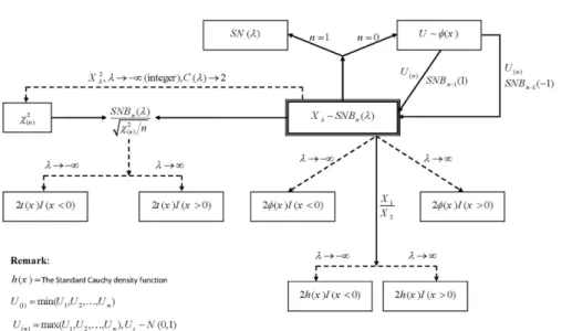
Figure 3 is depicted the asymptotic distributions together with the conditions of limiting. Limiting distributions, in Figure 3 and 4, are indicated with a dashed arrow. The standard normal and the binomial distribution play a very predomi-nant role in other distributions.

(Sharafi and Behboodian, 2008) have introduced the Balakrishnan skew-normal density (SNBn( )O ) and studied its properties. They defined the SNBn( )O

with integer nt1 by

( ; ) ( ) ( ) n( ), , ,

n n

f x O c O I x ) Ox x O\n] (5)

where the coefficient cn( )O is given by

1 1

( ) ,

( ( ))

( ) ( )

n _{n n}

c

E U

x x dx

O

I

f

f ) O ) O

³

where (0,1)UN .

An special case arises when n 1 and ( ) 2c_n O which gives the skew-normal

density (SN( ))O , see (Azzalini, 1985).

The probability distribution of the Balakrishnan skew-normal density and its relationships of the other distributions are also discussed. The most important properties of SNBn( )O are:

( )i SNB_n( )O is strongly unimodal,

1

1 1 2

1 1 3

( ) ( ) 2,

1 1

( ) sin ,

4 2

1 3

( ) sin ,

8 4

ii c

c

c O

O U

S

O U

S

ª º

« »

¬ ¼

ª º

« »

¬ ¼

Where U is denoted the correlation coefficient. For nt4, there is no closed form for ( )cn O . But some approximate values can be found in (Steck, 1962). The

bivariate case of SNBn( )O and the location and scale parameters are also pre-sented.

Figure 4 – The balakrishnan skew-normal density SNBn( )O .

3.CONCLUDING REMARKS

It is a reasonable assertion that all probability distributions are someway related to one another. In this paper, four diagrams summarize the most popular rela-tionships among the probability distributions. The relarela-tionships among the prob-ability distributions are one of the two classifications: transformation and limiting. Each diagram explains itself. The advantages of using these diagrams are: the stu-dent at the senior undergraduate level or beginning graduate level in statistics or engineering can use the diagrams to supplement course material. Besides, the re-searchers can use the diagrams for fasting search for the relationships among the distributions. These diagrams are just start points. Similar diagrams can be con-structed to summarize many statistical theorems such as: the characterizations of distributions based on; order statistics, Records and Moments, see (Gather et al., 1998).

Department of Math. YOUSRY ABDELKADER

Faculty of Science, Alexandria University, Egypt

Department of Math. ZAINAB AL-MARZOUQ

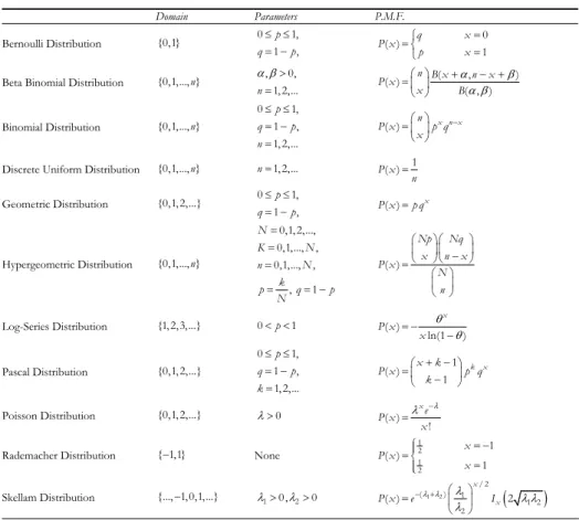
APPENDIX TABLE 1 Continues distribution PDF Parameters Domain

1_{(1 )} 1

( ) ( , ) x x f x B D E D E

0 , 0 D! E!

[0,1] Beta Distribution 1 (1 ) ( ) ( , ) x x f x B

D D E

D E

0 , 0 D! E!

[0, )f

Beta Prime Distribution

2 2 1 ( ) ( ) b f x x b

S K

,b 0 K\ !

(f f, ) Cauchy Distribution 2 2 1 2 1 1 2 2 ( ) ( ) n x n n

f x x e

* 0 n!

[0, )f

Chi Distribution 1 2 2 2 1 2 ( ) ( )2 n n x n x e f x * 0 n!

[0, )f

Chi-Squared Distribution 0 0 0 1 , ( ) ( ) 0 , x x

f x x x

x x

G ®­ _z

¯ 0

x \ 0

{ }x Degenerate Distribution 1 1 ( ) ( 1)! x n n x e f x n D D

1, 2,3, , 0 n "D!

[0, )f

Erlang Distribution

1 ( )

x

f x e D

D

0 T!

[0, )f

Exponential Distribution

1 2 2 2 2 2

1 2 1 2 2

1 1 2 1 2 2 2 ( ) , ( )

n n n

n n

n n

n n x

f x

B n n x

1 0, 2 0

n ! n !

[0, )f

F- Distribution 1 1 ( ) ( ) x x e

f x T D_T

T D

*

0 , 0 D! T!

[0, )f

Gamma Distribution

2

(ln ) / 2

1 ( )

2

x

f x e

x S

None (0, )f

Gibrat’s Distribution

1 ( )

x

x _e

f x e

D E D E E § · ¨ ¸ ¨ ¸ © ¹ ª º § · « » ¨ ¸ « » © ¹ « » ¬ ¼ 0 , E! D (f f, )

Gumbel Distribution

2 2_/

2 ( ) h h x

f x e S

S

0 h!

[0, )f

Half-Normal Distribution 2 1 2 21 2 2

( ) x

f x x e

Q Q Q * 0 Q!

(0, )f

Inverse Chi-Square Distribution

1

( ) x

f x TD x D eT D

*

0 , 0 D! T!

(0, )f

Inverse-Gamma Distribution

1 1

( ) a (1 a b)

f x ab x x

0 , 0 a! b!

[0,1] Kumaraswamy Distribution 1 ( ) 2 x b

f x e

b

P

0, b! P (f f, )

Laplace Distribution 2 3/ 2 ( ) 2 c x c e f x x S 0 c!

[0, )f

2 ( ) 1 x b x b e f x b e P P § · ¨ ¸ © ¹ § · ¨ ¸ © ¹ ª º « » « » ¬ ¼ 0, b! P (f f, )

Logistic Distribution

2

2

1 [ ln ]

( ) exp

2 2

x f x

x

P

V S V

§ · ¨ ¸ ¨ ¸ © ¹ 0, V! P [0, )f

Lognormal Distribution

2₂2

2

3

2 ( ) x ex a f x a S 0 a!

[0, )f

Maxwell Distribution 2 2 1 2 2 0 2 ( ) ( )

2 ! ( )

2 n n x k k n k x x e f x k k O O § · ¨ ¸

© ¹ f

*

¦

0, 0 n! O!

[0, )f

Noncentral

Chi-Squared Distribution

1 2 1

2 2 2

1 2 1 2 2 1 2 2 1

1 2 1 2

0 0 2 2 ( ) 2 1 ( ) 2 , ( )

k n l n k n

n n k l n n k l k l k l

n n x

f x

e B k l

n n x O O O O f f u ¦ ¦

1, , ,2 1 2 0

n n O O !

[0, )f

Noncentral F-Distribution

2 2 2 2

2 2

/ 2 2

2

3 1

1 1 2 22( ) 1 1 2 2 2( )

2 1 2

2 ₂

! ( )

2 ( )

2 1; ; 1; ;

( ) 1

n

n

n n

n x n x n x n x

n n

n n f x

e n x

x F F

n x n x

O O O O u *

­ ½

° ° ® ¾ * * ° ° ¯ ¿ 0, 0 n! O!

(f f, ) Noncentral Student’s t-Distribution 2 2 ( ) 2 1 ( ) 2 x

f x e

P V V S 2 _0,

V ! P (f f, )

Normal Distribution 0 1 ( ) k k k x f x x

0 0, 0

x ! k! 0

[x , )f

Pareto Distribution 1 1 ( ) ( ) x x

f x e

P D

T

P D T T

§ · _¨ ¸ © ¹ § · ¨ ¸

* © ¹

, 0, T D! P [0, )f

Pearson Type III Distribution

2 2 2 2 ( ) x x e

f x V

V

0 V!

[0, )f

Rayleigh Distribution 2 2 2 2 2 2 ( ) x o x x

f x e l

Q V Q V V _{§ ·} ¨ ¸ © ¹

0 , 0 V! Q!

[0, )f

Rice Distribution 2 2 1 ( ) 2 x

f x e

S

None (f f, )

Standard Normal Distribution

1 2 1 2 2 2 ( )

(1 / )n

n n

f x

nS x n

*

*

0 n!

(f f, ) Student’s t-Distribution 2( ) ( )( ) ( ) 2( ) ( )( ) x a

a x c b a c a f x

b x

c x b b a b c

­ _{d d}

°

°

®

° _{d d}

°

¯

a c b [ , ]a b

Triangular Distribution 1 ( ) f x b a , a b [ , ]a b

Uniform Distribution

1/ 2 2

3 2

( )

( ) exp

2 2 x f x x x O P O S P

ª º

ª º

« »

« »

¬ ¼ «¬ »¼

0, 0 O! P!

(0, )f

Wald Distribution

1

( )

x

f x x e

E E D E E D § · ¨ ¸ © ¹ , 0

D E!

[0, )f

TABLE 2 Discrete distribution P.M.F. Parameters Domain 0 ( ) 1 q x P x p x ­ ® ¯ 0 1, 1 , p q p d d {0,1} Bernoulli Distribution ( , ) ( ) ( , )

n B x n x

P x x B D E D E § · ¨ ¸ © ¹ , 0, 1, 2,... n D E!

{0,1,..., }n Beta Binomial Distribution

( ) n x n x

P x p q

x § · ¨ ¸ © ¹ 0 1, 1 , 1, 2,... p q p n d d

{0,1,..., }n Binomial Distribution 1 ( ) P x n 1, 2,... n {0,1,..., }n

Discrete Uniform Distribution

( ) x

P x p q

0 1, 1 , p q p d d {0,1, 2,...} Geometric Distribution ( ) Np Nq

x n x

P x N

n

§ ·§ ·

¨ ¸¨ ¸

© ¹© ¹

§ · ¨ ¸ © ¹ 0,1, 2,..., 0,1,..., , 0,1,..., , , 1 N K N n N k

p q p

N

{0,1,..., }n Hypergeometric Distribution ( ) ln(1 ) x P x x T T

0 p 1 {1, 2,3,...} Log-Series Distribution 1 ( ) 1 k x x k

P x p q

k § · ¨ ¸ © ¹ 0 1, 1 , 1, 2,... p q p k d d {0,1, 2,...} Pascal Distribution ( ) ! x e P x x O O 0 O! {0,1, 2,...} Poisson Distribution 1 2 1 2 1 ( ) 1 x P x x ­ ° ® °¯ None { 1,1} Rademacher Distribution 1 2 / 2

( ) 1

1 2 2

( ) 2

x x

P x e O O O I _{O O}

O

§ ·

¨ ¸

© ¹

1 0, 2 0

O ! O !

{..., 1,0,1,...}

Skellam Distribution

REFERENCES

A. AZZALINI (1985), A class of distributions with includes the normal ones, “Scandinavian journal

of statistics”, 12, pp. 171-178.

E. L. CROW, K. SHIMIZU (1988), Lognormal distributions: Theory and Applications, Marcel Dekker,

New York.

U. GATHER, U., KAMPUS, andN. SCHWEITZER (1998), Characterizations of distributions via identically

distributed functions of order statistics, In: Balakrishnan, N., and Rao, C. ed., “Handbook of

Statistics”, 16, Elsevier Science, pp. 257-290.

N. JOHNSON, S. KOTZ and N. BALAKRISHNAN (1994), Continuous univariate distributions, Vol. 1,

2nd ed. Wiley, New York.

N. JOHNSON, S. KOTZ and N. BALAKRISHNAN (1995), Continuous univariate distributions, Vol. 2,

2nd ed., Wiley, New York.

I. KOTLARSKI (1962), On group of n independent random variables whose product follows the beta

distri-bution, “Collog. Math. IX Fasc.”, 2, pp. 325-332.

W. KRYSICKI (1999), On some new properties of the beta distribution, “Statistics & Probability

L. LEEMIS (1986), Relationships among common univariate distributions, “The American

Statisti-cian”, 40, pp. 143-146.

M. SHARAFI, J. BEHBOODIAN (2008), The Balakrishnan skew-normal density, “Statistical Papers”,

49, pp. 769-778.

J.W. RIDER (2004), Probability distribution relationships, http://www.jwrider.com.

H. A. TAHA (2003), Operations Research: An introduction, 3rd ed, Macmillan Publishing Co.

SUMMARY

Probability distribution relationships