Sensorless finite control set model predictive control for IPMSM drives

Abstract —This paper investigates the feasibility of a sensorless field oriented control (FOC) combined with a finite control set model predictive current control (FCS-MPC) for an interior permanent magnet synchronous motor (IPMSM). The use of a FCS-MPC makes the implementation of most of the existing sensorless techniques difficult due to the lack of a modulator. The proposed sensorless algorithm exploits the saliency of the motor and the intrinsic higher current ripple of the FCS-MPC to extract position and speed information using a model-based approach. This method does not require the injection of additional voltage vectors or the periodic interruption of the control algorithm and consequently it has no impact on the performance of the current control. The proposed algorithm has been tested in simulation and validated on an experimental set-up, showing promising results.

I. INTRODUCTION

ERMANENT magnet synchronous motors (PMSMs), compared to other motor types like induction motors, offer several advantages in the field of variable-speed AC drives. They have higher efficiency, higher performance, compact construction, higher torque per volume ratio. In particular, interior permanent magnet synchronous motors (IPMSMs) provide an increased efficiency by taking advantage of the reluctance torque and of the constant-power operation mode obtainable by flux-weakening the machine.

To achieve high performance, PMSMs are usually controlled with FOC; hence position and speed information are needed and typically measured with a position sensor such as an encoder. Additionally, IPMSMs allow simpler sensorless rotor position estimation using either back electromagnetic force (EMF) or the saliency effect. The possibility of avoiding the installation of a position sensor results in the elimination of a fragile component from the system and in a significant reduction of the overall drive cost and size. This explains the numerous attempts made to eliminate the position sensor. Sensorless control techniques can be divided in two main groups. The first one is represented by the fundamental excitation techniques [1-6], which estimate the rotor speed and position exploiting the back electromotive force generated by the

permanent magnet. The second one corresponds to the saliency tracking techniques [7-14], which, injecting a persistent high-frequency signal, exploit the rotor anisotropy to reconstruct its position. The former methods do not require any additional signal injection, but, in case of techniques based on the estimation of the back electromotive force (EMF), they hardly operate at low speeds and surely not at standstill due to the lack of useful information. The latter methods have the advantage of working also at standstill so avoiding the use of open loop control strategies for starting the motor, but require the injection of additional high-frequency signals leading to increased torque ripple, noise and losses. The INFORM method [5], for example, requires periodic interruptions of the modulation/control and the injection of a particular set of voltage vectors for generating a current transient sufficiently large to appreciate the inductance variation with position. Many of the previously described sensorless techniques cannot be immediately used in conjunction with a FCS-MPC as a consequence of its different way of operation with respect to a traditional linear controller and the absence of a modulator. FCS-MPC is a relatively new and powerful control approach that has received, in recent years, a great interest from the academic community [15-20]. It uses the model of the system to predict its future states subject to every possible control action. The best control action is then chosen by minimizing a cost function. This approach permits to remove the modulator, reduces the control sample time and decreases consequently the response time. This advantage becomes however a drawback if the drive has to be controlled without a position sensor. The absence of a modulator and consequently of a reference voltage signal makes the previously described sensorless methods difficult to be implemented without deep modifications to them and/or to FCS-MPC itself. For example, in [21] a back-EMF observer has been combined with a FCS-MPC. For estimating the rotor position and speed, a simple PLL-structure, derived from the motor mathematical model and which tracks the flux linkage vector, has been chosen to limit the computational burden and maintain the short sample time and the high bandwidth, which are contradistinctive features of the MPC.

This paper investigates the feasibility of implementing a sensorless control for the whole motor speed range in conjunction with a FCS-MPC. The absence of a modulator in the FCS-MPC makes the injection or reconstruction of a continuous control input very difficult since the controller operates in the discrete space of the inverter states. For this reason, the implementation of sensorless techniques based on the injection of continuous (usually sinusoidal) signal is not straightforward in conjunction with FCS-MPC. A different approach is therefore proposed in this work, in order to

Luca Rovere, Andrea Formentini

, Member, IEEE,

Alberto Gaeta

, Member, IEEE,

Pericle

Zanchetta

, Senior Member, IEEE,

Mario Marchesoni

, Member IEEE

P

Sensorless Finite Control Set Model Predictive

Control for IPMSM Drives

Manuscript received June 11, 2015; revised November 14, 2015 and February 16, 2016; accepted March 22, 2016.

L. Rovere, A. Formentini and P. Zanchetta are with the Department of Electrical and Electronic Engineering, The University

of Nottingham, Nottingham, NG7 2RD, U.K. (email:

[email protected], [email protected],

[email protected] (corresponding author)). Alberto Gaeta is with reDrives S.r.l., via Tommaso Fazello 5, Lentini, Italy (email: [email protected]).

combine FCS-MPC to a sensorless algorithm. It is based on the mathematical IPMSM model and allows the estimation of the rotor position starting from the current measurements, the knowledge of the voltages applied to the motor and its parameters. Although being a model-based method, the proposed approach allows the estimation of the rotor position at standstill by exploiting the higher current ripple which typically is considered a drawback of the FCS-MPC. Being the ripple amplitude approximately unaffected by the speed, the rotor position information extracted from the current ripple is also used at higher speeds. Moreover, due to the particular way the mathematical model is rearranged and used, the back-EMF is not considered at all for the rotor position estimation and so all the problems deriving from its large variation with temperature are eliminated. Since reference voltages are used in place of measured quantities to avoid the need for costly, bulky and fragile voltage sensors, an adequate knowledge of the voltage effectively applied to the motor is required. For this reason dead-time compensation has been also implemented to reduce the voltage distortion introduced by the inverter to acceptable levels. The main contribution of the proposed paper is investigating the feasibility of implementing the emerging FCS-MPC technique in a drive application without position sensor. The absence of a modulator makes the implementation of the standard sensorless control techniques a difficult task. For this reason a new sensorless algorithm that takes advantage of the bigger current ripple generated by FCS-MPC is proposed.

The paper is organized as follows. Section II describes in details the proposed sensorless method, Section III presents the FCS-MPC algorithm used for the current control loop, Section IV and V show the obtained simulation and experimental results and finally section VI reports the conclusions.

II. SENSORLESS ALGORITHM

The machine inductances in a stationary reference frame are dependent from the rotor position due to the magnetic saliency. This feature is exploited in the proposed algorithm in order to estimate the rotor position θ from the measurements of electrical quantities. The mathematical model for an IPMSM in the α-β reference frame is:

[𝑉_𝑉𝛼 𝛽] = [

𝑅𝑠 0

0 𝑅𝑠] [

𝐼𝛼 𝐼𝛽] +

𝑑 𝑑𝑡 [

𝜆𝛼

𝜆𝛽] (1)

where

[𝜆_𝜆𝛽𝛼] = 𝐿𝛼𝛽[𝐼_𝐼𝛼

𝛽] + 𝜆𝑚 [ 𝑠𝑖𝑛(𝜗) − 𝑐𝑜𝑠(𝜗)]

(2)

𝐿𝛼𝛽= [1 0_{0 1}] 𝐿𝐴+ [− 𝑐𝑜𝑠(2𝜗) 𝑠𝑖𝑛(2𝜗)_{𝑠𝑖𝑛(2𝜗) 𝑐𝑜𝑠(2𝜗)}] 𝐿𝐵

𝐿𝐴=𝐿𝑑 + 𝐿𝑞

2 𝐿𝐵 =

𝐿𝑑− 𝐿𝑞 2

𝑉𝛼, 𝑉𝛽 are the motor voltages, 𝐼𝛼, 𝐼𝛽 the machine currents and

𝜆𝛼, 𝜆𝛽 the flux linkages. θ is the rotor electrical position, 𝜆𝑚 is

the peak flux linkage established by the magnets, 𝑅𝑠 is the stator resistance and 𝐿𝑞, 𝐿𝑑 are q- axis and d-axis inductance in the rotor reference frame.

The model in (2) has been discretized using the Euler discretization method. The discretization around a generic time instant k leads to the following equations:

[𝐼_𝐼𝛼𝑘+1 𝛽𝑘+1] = Fk[

𝐼_𝛼𝑘

𝐼_𝛽𝑘] + Hk[ 𝑉_𝛼𝑘 𝑉_𝛽𝑘]

+𝜔𝑘𝑇𝑠𝜆𝑚

𝐿𝑞 [

− cos(𝜃𝑘) sin(𝜃𝑘) ]

(3)

where 𝐹𝑘∈ ℜ2𝑥2 and 𝐻𝑘∈ ℜ2𝑥2 are terms dependent on 𝑅𝑠,

𝐿𝑞, 𝐿𝑑 , cos(2θk), 𝑠𝑖𝑛(2𝜃𝑘), the system sample time 𝑇𝑠 and

the electrical speed 𝜔𝑘, as better described in the Appendix, while the subscript k denotes the time instant.

Applying a time shift of one sample ahead to (3)

[𝐼_𝐼𝛼𝑘+2

𝛽𝑘+2] = Fk+1[ 𝐼_𝛼𝑘+1

𝐼_𝛽𝑘+1] + Hk+1[ 𝑉_𝛼𝑘+1 𝑉_𝛽𝑘+1]

+𝜔𝑘+1𝑇𝑠𝜆𝑚

𝐿𝑞 [

− cos(𝜃𝑘+1) sin(𝜃𝑘+1) ]

(4)

𝐹𝑘+1 ∈ ℜ2𝑥2 and 𝐻𝑘+1∈ ℜ2𝑥2 have the same expression of 𝐹𝑘

and 𝐻𝑘 but are dependent on 𝑐𝑜𝑠(2𝜃𝑘+1) and 𝑠𝑖𝑛(2𝜃𝑘+1) where 𝜃_𝑘+1= 𝜃_𝑘+ 𝜔_𝑘𝑇_𝑠.

Subtracting (3) and (4), assuming 𝜔𝑘 = 𝜔𝑘+1 and rearranging the equations the following system is obtained

𝐾𝑘+2= [_{−𝑠𝑖𝑛(2𝜃𝑘}𝑐𝑜𝑠(2𝜃𝑘)_{) 𝑐𝑜𝑠(2𝜃}𝑠𝑖𝑛(2𝜃𝑘)

𝑘)] 𝑁𝑘+2+ [

𝑓1

𝑓2] (5)

with

𝑓1=

𝑇𝑠𝜆𝑚𝜔𝑘

𝐿𝑞 𝑐𝑜𝑠(𝜃𝑘) (1 − 𝑐𝑜𝑠(𝜔𝑘𝑇𝑠)) + 𝑇𝑠𝜆𝑚𝜔𝑘

𝐿𝑞 𝑠𝑖𝑛 (𝜃𝑘)𝑠𝑖𝑛 (𝜔𝑘𝑇𝑠) 𝑓2=

𝑇𝑠𝜆𝑚𝜔𝑘

𝐿𝑞 𝑐𝑜𝑠(𝜃𝑘) 𝑠𝑖𝑛 (𝜔𝑘𝑇𝑠)

− 𝑇𝑠𝜆𝑚𝜔𝑘

𝐿𝑞 𝑠𝑖𝑛 (𝜃𝑘) (1 − 𝑐𝑜𝑠(𝜔𝑘𝑇𝑠))

(6)

where 𝐾_𝑘+2∈ ℜ2𝑥1 and 𝑁_𝑘+2 ∈ ℜ2𝑥1 are dependent on the parameters of the system 𝑇𝑠, 𝑅𝑠, 𝐿𝑞, 𝐿𝑑 , on the rotor speed 𝜔𝑘

and on measurements 𝐼_𝛼𝑘, 𝐼_𝛽𝑘, 𝐼_𝛼𝑘+1, 𝐼_𝛽𝑘+1, 𝐼_𝛼𝑘+2, 𝐼_𝛽𝑘+2, 𝑉_𝛼𝑘,

𝑉_𝛽𝑘, 𝑉_𝛼𝑘+1, 𝑉_𝛽𝑘+1. FCS-MPC generates a lower average switching frequency compared to the controller sampling frequency (4 to 20 times smaller in the proposed control scheme, depending on the motor speed). For this reason it is possible to assume the term ωkTssufficiently small, being 𝑇𝑠

two sample, (5) reduces to

𝐾𝑘= [_{−𝑠𝑖𝑛(2𝜃𝑘−2}𝑐𝑜𝑠(2𝜃𝑘−2)_{) 𝑐𝑜𝑠(2𝜃}𝑠𝑖𝑛(2𝜃𝑘−2)

𝑘−2)] 𝑁𝑘 (7)

From (5) it can be noticed that vector 𝐾_𝑘+2 is the result of the rotation of vector 𝑁𝑘+2 by 2𝜃𝑘. At each control step it is then

possible to compute an estimation of the vector K as

𝐾̂𝑘= [

𝑐𝑜𝑠(2𝜃̂𝑘−2) 𝑠𝑖𝑛(2𝜃̂𝑘−2)

−𝑠𝑖𝑛(2𝜃̂𝑘−2) 𝑐𝑜𝑠(2𝜃̂𝑘−2)] 𝑁𝑘 (8)

where 𝜃̂_𝑘−2 is the estimated rotor position. Defining 𝜃_𝑘−2𝑒 as the error between the estimated electrical rotor position and the real one, it is possible to note from Fig. 1 that 2𝜃_𝑘−2𝑒 is also the angle between the vectors 𝐾𝑘 and 𝐾̂𝑘.

2𝜃𝑘−2𝑒 ∶= 2𝜃𝑘−2− 2𝜃̂𝑘−2 (9)

The cross product between 𝐾_𝑘 and 𝐾̂_𝑘 can be expressed as follows

𝐾𝑘× 𝐾̂𝑘 = |𝐾𝑘| |𝐾̂𝑘| 𝑠𝑖𝑛 (2𝜃𝑘−2𝑒 ) (10)

However it can also be expressed in the i, j, k coordinate notations has

𝐾𝑘× 𝐾̂𝑘= 𝑑𝑒𝑡 ([

𝑖 𝑗 𝑘

𝐾_1𝑘 𝐾_2𝑘 0

𝐾̂_1𝑘 𝐾̂_2𝑘 0 ]) =

= 0 𝑖 − 0 𝑗 + (𝐾_1𝑘𝐾̂_2𝑘− 𝐾_2𝑘𝐾̂_1𝑘)𝑧

(11)

Equating the right side of (10) and (11)

|𝐾𝑘| |𝐾̂𝑘| 𝑠𝑖𝑛(2𝜃𝑘−2𝑒 ) = 𝐾_1𝑘𝐾̂_2𝑘− 𝐾_2𝑘𝐾̂_1𝑘 (12)

It is therefore possible to compute the sine of the angle between 𝐾𝑘 and 𝐾̂𝑘 solving (12) for 𝑠𝑖𝑛(2𝜃_𝑘−2𝑒 )

𝑠𝑖𝑛(2𝜃𝑘−2𝑒 ) =

𝐾̂_2𝑘𝐾_1𝑘− 𝐾̂_1𝑘𝐾_2𝑘

√(𝐾̂_1𝑘2+ 𝐾̂_2𝑘2) (𝐾_1𝑘2_{+ 𝐾}

2𝑘2)

(13)

where

𝐾𝑘 = [𝐾_𝐾1𝑘

2𝑘] 𝐾̂𝑘 = [

𝐾̂_1𝑘

𝐾̂_2𝑘] (14)

It is worth to note that terms 𝐾𝑘 and 𝑁𝑘 depend on system inputs (voltages) and outputs (currents) at different sampling time. Analyzing their structure it can be noted that, in a perfect steady state condition where both inputs and outputs do not change, these terms are equal to zeros and the estimation is no longer possible. This is coherent with equation (5) , which has been derived from the subtraction of system equation at different sampling time, and reflects the persistent excitation principle [22]. Fortunately, systems controlled with commutated inverters never reach a complete steady state condition: the discontinuous voltage generated by the inverter creates a current ripple with variable amplitude depending on different system parameters. Using a PWM modulation technique however, steady state current variation is very small, especially at low speed. This results in a small absolute value of parameters 𝐾𝑘 and 𝑁𝑘 that cause a very noisy and often unusable position estimation. For this reason a signal injection is usually adopted for position estimation at low or zero speed in order to increase the current variation. FCS-MPC produce a bigger current ripple at low speed compared to PWM modulation techniques in favor of a lower switching frequency. This ripple results in bigger 𝐾𝑘 and 𝑁𝑘 modules

permitting therefore a more accurate position estimation without the need of a signal injection.

To estimate the rotor speed and position using the information of (13), an observer of the mechanical system has been implemented [23]. The observer used in this paper is in the form

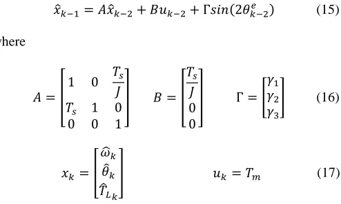
𝑥̂𝑘−1= 𝐴𝑥̂𝑘−2+ 𝐵𝑢𝑘−2+ Γ𝑠𝑖𝑛(2𝜃𝑘−2𝑒 ) (15)

where

𝐴 = [1 0

𝑇𝑠 𝐽

𝑇𝑠 1 0

0 0 1

] 𝐵 = [

𝑇𝑠 𝐽 0 0

] Γ = [

𝛾1 𝛾2 𝛾3

] (16)

𝑥𝑘= [ 𝜔̂𝑘

𝜃̂𝑘 𝑇̂_𝐿𝑘

] 𝑢𝑘 = 𝑇𝑚 (17)

J is the system inertia, 𝜔̂ is the estimation of the electrical speed, 𝑇𝑚 is the electromagnetic torque and 𝛾𝑖, 𝑖 = 1,2,3, are

the observer gains. The observer has been extended [24] to estimate also 𝑇̂𝐿, that is the estimation of the load torque

applied to the motor shaft.

It should be noted that the observer described by (15) is nonlinear due to the sinusoidal correction term 𝑠𝑖𝑛(2𝜃_𝑘−2𝑒 );

the asymptotic stability of this observer has been however demonstrated in [25].

The algorithm can be summarized as follows:

1. At kth time instant the new currents are measured and the vectors 𝑁_𝑘 and 𝐾_𝑘 are computed

2. The vector 𝐾̂𝑘 is computed according to (8)

3. The sine of the position error is computed as shown in (13)

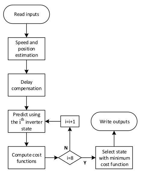
4. The new observer state is updated according to (15) III. FIELD ORIENTED CONTROL WITH FCS-MPC Power converters have an intrinsic finite number of states, depending on the power devices on-off combinations, each corresponding to a different possible control action. FCS-MPC takes advantage of this propriety to predict the behavior of the controlled system for every possible converter configurations over a few sample time instants. The optimal control actions are chosen minimizing a cost function that depends on both the predicted state and the reference signals. Only the first optimal control action is applied and at the next sample instant the procedure is repeated. FCS-MPC is a very powerful control strategy that permits to regulate different system variables with a single control action simply designing conveniently the cost function.

Fig. 2 shows the flow chart of the FCS-MPC utilized in this paper. At the beginning of each sample time, the motor currents and DC bus voltage are sampled. Subsequently the new speed and position are estimated as explained in section II. The short sampling period and the high computational cost required by the FCS-MPC imply that the new control action is available to be applied only at the beginning of the next sampling instant. This generates a sample delay in the control

loop that must be compensated. To accomplish this task the system state at the (k+1)th sampling period has been predicted using the optimal control action obtained at the (k-1)th sampling period [26]. The system state at the (k+2)th sampling period is then predicted for each of the 8 possible control actions.

The system has been modelled in the synchronous reference frame by the following equations

𝐼̇𝑑= − 𝑅𝑠

𝐿𝑑𝐼𝑑+

𝐿𝑞𝐼𝑞𝜔

𝐿𝑑 +

𝑉𝑑 𝐿𝑑 𝐼̇𝑞 = −

𝐿𝑑𝐼𝑑𝜔

𝐿𝑞 −

𝑅𝑚

𝐿𝑞 𝐼𝑞−

𝜑𝑛𝑝

𝐿𝑞 𝜔 +

𝑉𝑞 𝐿𝑞

(18)

The system has been subsequently discretized resulting in

𝐼_𝑑𝑘+1= −𝑅𝑠 𝐿𝑑𝐼𝑑𝑘+

𝑇𝑠𝐿𝑞𝜔

𝐿𝑑 𝐼𝑞𝑘+

𝑇𝑠 𝐿𝑑𝑉𝑑𝑘

𝐼_𝑞𝑘+1= −𝑅𝑚

𝐿𝑞 𝐼𝑞𝑘− 𝑇𝑠𝐿𝑑𝜔

𝐿𝑞 𝐼𝑑 𝑘− 𝑇𝑠𝜆𝑚

𝐿𝑞 𝜔 +

𝑇𝑠 𝐿𝑞𝑉𝑞𝑘

(19)

The objective in a FOC control of a PMSM is to control the 𝐼𝑑

and 𝐼𝑞 currents to their reference values. For this reason the following cost function has been chosen

𝑐𝑓= (𝐼𝑑∗− 𝐼𝑑 𝑘+2)

2

+ (𝐼𝑞∗_{− 𝐼}

𝑞𝑘+2)

2

(20)

where 𝐼𝑞∗ and 𝐼_𝑑∗ are the reference currents.

The cost function (20) is computed 8 times, once for each of the 8 predictions previously described. The cost function with minimum value is selected as optimal and the related inverter state is then chosen and applied during the next sampling period.

Analytical stability analysis of systems based on FCS-MPC is a challenging task due to the intrinsic discontinuity of the controller and therefore is still an open topic in literature. In the presented work however, system stability has been verified empirically trough simulative and experimental tests. As it will be shown in the next sections, the complete control loop demonstrates good and stable behaviors in both low and high speed working condition.

A. Ripple and switching frequency analysis

Speed and position estimation

Delay compensation

Predict using the ith inverter

state

Write outputs

Compute cost

functions i=8 i=i+1

Select state with minimum

cost function Read inputs

Y N

Fig. 2 – FCS-MPC flowchart.

T

FCS-MPC PI

-+



M

Sensorless

I

Vvector



ˆ

ˆ

VSI

As opposed to standard SVM-based methods, FCS-MPC produces a variable switching frequency. It is however possible to introduce an average switching frequency (ASF) as the average number of turn-on and turn-off of a single inverter switch in a second. TABLE I shows the ASF and current Total Harmonic Distortion (THD) using FCS-MPC computed through a simulative model at different motor speeds. It is possible to notice from the table that the ASF increases in a proportional way with the motor speed. This behavior is also reflected on the current distortion resulting, as opposed to PWM-based techniques, in an almost constant ripple over the whole speed range.

IV. SIMULATION ANALYSIS

The proposed method has been firstly analyzed in simulation. Fig. 3 shows the overall control structure. The FCS-MPC block implements the controller described in the previous Section while the sensorless block implements the proposed algorithm for the estimation of the rotor position described in Section II. Different research works have appeared in literature proposing the speed loop embedded within the FCS-MPC [18, 19, 27, 28]. However, the proposed sensorless position detection is not affected by the control strategy used to regulate the motor speed. Therefore, for the sake of clarity and simplicity, a standard proportional integral (PI) controller has been used for the speed loop. In this work, no current profiling technique like Maximum Torque Per Ampere (MTPA) has been

implemented and the torque is generated using only 𝐼𝑞, while

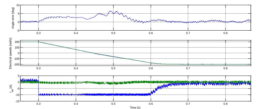
𝐼𝑑 is controlled to zero. The parameters used to simulate the model are reported in TABLE II. The observer gain Γ has been set placing the closed loop poles of the linearized system (15) in a Butterworth configuration. The frequency of such poles should be selected as a compromise choice between a fast transient response and a noisy estimation: a larger frequency results in a faster transient response, but also in a noisier estimation. In this work an observer bandwidth of about 10 Hz has been used. Fig. 4 shows the response of the proposed algorithm to a speed variation from 200 to -200 electrical rad/s. The 𝐼_𝑞 current has been saturated to 10 A accordingly to the maximum RMS current of the motor used in the experimental set-up in order to have consistent results between simulation and experimental tests. It can be noticed how the error in the rotor position estimation increases during each transient, but remains limited so allowing a proper control of the machine.

A. Robustness analysis

In order to verify the robustness of the proposed system to parameters uncertainties a simulative robustness analysis has been carried out. In a real application both the stator resistance and the inductance can vary. The first one is mainly affected by temperature with an uncertainty up to 30% while the latter

Fig. 4 – Simulation results - Speed reversal. Top: error between real and estimated electrical rotor angle. Middle: real (blue) and estimated (green) electrical rotor speed. Bottom: 𝐼𝑑 (green) and 𝐼𝑞 (blue) currents.

0.3 0.4 0.5 0.6 0.7 0.8

-5 0 5 10

A

n

g

le

e

rr

o

r

[d

e

g

]

0.3 0.4 0.5 0.6 0.7 0.8

-200 -100 0 100 200

E

le

c

tr

ic

a

l

s

p

e

e

d

s

[

ra

d

/s

]

0.3 0.4 0.5 0.6 0.7 0.8

-15 -10 -5 0 5

Iqd

[

A

]

Time [s]

TABLEI

FCS-MPCPHASECURRENTTHDANDAVERAGE

SWITCHINGFREQUENCY

Angular speed (rad/s)

Current THD (%)

Average Switching Frequency (Hz)

5 6.56 1061 50 7.19 2838 100 7.29 4907 200 7.40 7580

TABLEII

SYSTEMPARAMETERS

Name Value Unit

Motor rated current 7 ARMS

𝐿𝑞 6.486 [mH]

𝐿𝑑 4.9254 [mH]

R 1.35 [Ω]

𝜆𝑚 0.22 [V s]

p 4 -

𝐽 31.685 [g m2]

can change due to ferromagnetic saturation. The test, whose results are reported in Fig. 4, has been therefore performed again with a variation of the system parameters with respect to the ones used in the controller. Fig. 5 and Fig. 6 show a speed reversal test with a 30% resistance variation and 10% inductance variation, respectively. As it can be noticed from the figures, in these conditions the estimation becomes noisier. However, the system is still stable and the controller is able to regulate the system states as required.

The simulative analysis has also highlighted the need of compensating the voltage distortion introduced by the dead-time of the switches [29]. In fact, to ensure proper operation of the inverter, the bridge shoot through should be always avoided, since it will cause additional losses or even thermal runaway. As a result, failure of IGBT devices and even of the whole inverter is possible. In order to avoid bridge shoot through it is always recommended to add a “dead time” into the control scheme.Usually several micro seconds are required for the dead-time which are no longer ignorable in the inverter modelling. The proposed sensorless algorithm needs the real applied voltage by the inverter at each sample time. Neglecting a possible distortion introduced by the dead-time results in inaccurate and useless position estimation. For this reason, the dead-time compensation algorithm proposed in [30] has been used in both simulative and experimental results.

Fig. 7 shows the state of the higher and lower gate signals of the jth inverter leg and the output phase voltage 𝑣𝑗0 of the inverter in the case of a positive phase current. When the upper IGBT turns-off the current continue to flow through the lower diode, delaying the change of the output voltage. As soon as the lower IGBT is turned on the output voltage switches to 𝑉𝐷𝐶₂ . To obtain a good position estimation, the output voltage distortion is therefore compensated considering as applied voltage its mean value over a sample time. As the voltage error introduced by the dead-time is constant, if absolute voltage values are considered, its relative influence is lower at high speeds and higher at low speeds, being the

voltage amplitude applied to motor terminals nearly proportional to the motor speed. Therefore dead-time compensation is needed especially at low speed operations.

V. EXPERIMENTAL RESULTS

The proposed method has been finally tested on an experimental set-up. It is composed by an IPMSM coupled with a DC motor as shown in Fig. 8. The IPMSM is fed by a two level IGBT converter. The control has been implemented on a C6713 Texas Instruments DSP coupled with a Microsemi A3P400 FPGA, with a sample time of 25 𝜇𝑠. The mechanical and electrical system parameters have been identified with the approach proposed in [31, 32] and are shown in TABLE . The sensorless methods based on the rotor saliency can identify the

Fig. 5 – Simulation results - Speed reversal with an increment of R of 30%. Top: real (blue) and estimated (green) electrical rotor speed. Middle: error between real and estimated electrical rotor angle. Bottom: 𝐼𝑑 (green) and 𝐼𝑞 (blue) currents.

Fig. 6 – Simulation results - Speed reversal with a decrement of L of 10%. Top: real (blue) and estimated (green) electrical rotor speed. Middle: error between real and estimated electrical rotor angle. Bottom: 𝐼𝑑 (green) and 𝐼𝑞 (blue) currents.

Fig. 7 – State of the high (SjH) and low (SjL) IGBT of the jth leg of

initial rotor electrical position with an uncertainty of 180 degree. Different initial rotor polarity estimation procedures have been proposed in literature [33, 34]. They can be easily applied with the proposed sensorless algorithm without the necessity of any modification. For this reason the problem of identifying the initial rotor polarity is not addressed in this paper and it is assumed to be known. At system power up, the controller is started in only current closed loop and a value of

𝐼𝑑 current is injected to allow the estimator to lock to the rotor angle. Fig. 9 shows the transient of the error between rotor position estimation (arbitrary set equal to 0 at system start-up) and the real rotor position (in the proposed test equal to 60°). During the test the 𝐼_𝑑 current has been set equal to 3 A. It is evident how the estimated electrical position rapidly

converges to the actual one. The system is subsequently run in speed closed loop mode and is thereafter ready for operation. Fig. 10 shows a speed reversal from a speed of 50 rad/s to -50 rad/s where it is possible to note a good match between the real and estimated angle for the whole speed transient. To evaluate the robustness of the proposed method to higher speed, Fig. 11 shows the steady state behavior of the system at nominal speed, namely 150 rad/s. The system has been also tested at 5 rad/s to validate its reliability at low speed as shown in Fig. 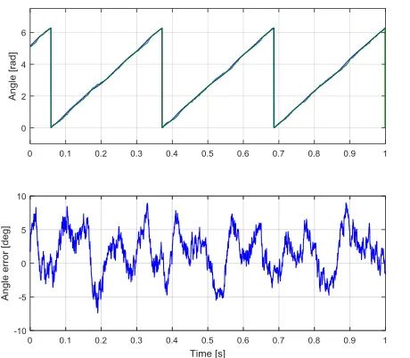12.

Finally Fig. 13 and Fig. 14 show the rotor position estimation error with the machine rotating at a constant speed of 50 and 5 mechanical rad/s respectively, with the nominal load torque applied. This test is particularly useful to evaluate the

Fig. 8 – Experimental set-up: two level inverter (green circle), control platform (red circle) and motors.

Fig. 9 – Experimental results - Observer transient at system start-up. Top: error between real and estimated electrical rotor angle. Bottom: 𝐼𝑑 (green) and 𝐼𝑞 (blue) currents.

0 0.2 0.4 0.6 0.8 1 1.2 1.4

-80 -60 -40 -20 0 20

A

n

g

le

e

rr

o

r

[d

e

g

]

0 0.2 0.4 0.6 0.8 1 1.2 1.4

-2 0 2 4 6 8

Iqd

[

A

]

Time [s]

Fig. 10 – Experimental results - Speed inversion. From top to bottom: real (blue) and estimated (green) electrical rotor angle; error between real and estimated electrical rotor angle; real (blue) and estimated (green) electrical rotor speed; 𝐼𝑑 (green) and 𝐼𝑞 (blue) currents.

0.1 0.2 0.3 0.4 0.5 0.6 0.7 0.8 0

2 4 6

A

n

g

le

[

ra

d

]

0.1 0.2 0.3 0.4 0.5 0.6 0.7 0.8 -10

-5 0 5 10

A

n

g

le

e

rr

o

r

[d

e

g

]

0.1 0.2 0.3 0.4 0.5 0.6 0.7 0.8 -200

0 200

E

le

c

tr

ic

a

l

s

p

e

e

d

s

[

ra

d

/s

]

0.1 0.2 0.3 0.4 0.5 0.6 0.7 0.8 -20

-10 0 10

Iqd

[

A

]

robustness of the proposed algorithm against inductance variation due to flux saturation. Even if a slight offset appears in the position estimation, this test demonstrates the robustness of the proposed method to inductance changes.

VI. CONCLUSION

This paper introduces a new model based algorithm to estimate the rotor position of an IPMSM using a FCS-MPC so to allow drive sensorless control. This new approach also exploits the characteristic current ripple naturally generated by FCS-MPC to estimate the rotor position in every load and speed condition without the necessity to superimpose any additional voltage or current signal. This work therefore demonstrates the feasibility of sensorless control even when using a Finite control set Model predictive drive control approach and without the use of a standard modulation system. The good simulation and experimental results show

the potentiality of the proposed method. APPENDIX

In the following the omitted terms of (3)-(5)are reported.

𝐹𝐾= [𝐹_𝐹1 𝐹2 3 𝐹4] 𝐹1= 1 −

𝑅𝑠𝑇𝑠

𝐿𝑑𝐿𝑞 (𝐿1+ 𝐿2cos(2𝜃𝑘)) − 𝜔𝑘𝑇𝑠

2𝐿𝑑𝐿𝑞𝐿3sin(2𝜃𝑘)

𝐹2= [ 𝑅𝑠𝑇𝑠

𝐿_𝑑𝐿_𝑞 𝐿2sin(2𝜃𝑘) − 𝜔𝑘𝑇𝑠

2𝐿_𝑑𝐿_𝑞 (𝐿3cos(2𝜃𝑘) + 4𝐿22)]

𝐹3= [ 𝑅𝑠𝑇𝑠

𝐿𝑑𝐿𝑞 𝐿2sin(2𝜃𝑘) + 𝜔𝑘𝑇𝑠

2𝐿𝑑𝐿𝑞 (−𝐿3cos(2𝜃𝑘) + 4𝐿2 2_)]

𝐹4= 1 − 𝑅𝑠𝑇𝑠

𝐿𝑑𝐿𝑞 (𝐿1− 𝐿2cos(2𝜃𝑘)) + 𝜔𝑘𝑇𝑠

2𝐿𝑑𝐿𝑞 𝐿3sin(2𝜃𝑘 )

(21)

𝐻𝐾= [𝐻_𝐻1 𝐻2 3 𝐻4] 𝐻1=

1

𝐿𝑑𝐿𝑞 𝑇𝑠 (𝐿1+ 𝐿2 cos(2𝜃𝑘) )

(22)

Fig. 11 – Experimental results - Steady state behaviour at 600 electrical rad/s. Top: real (blue) and estimated (green) rotor angle. Bottom: error between real and estimated rotor angle.

0.1 0.15 0.2 0.25 0.3 0.35 0.4 0

2 4 6

A

n

g

le

[

ra

d

]

0.1 0.15 0.2 0.25 0.3 0.35 0.4 -4

-2 0 2 4 6

A

n

g

le

e

rr

o

r

[d

e

g

]

Time [s]

Fig. 12 – Experimental results - Steady state behaviour at 5 mechanical rad/s. Top: real (blue) and estimated (green) rotor electrical angle. Bottom: error between real and estimated rotor electrical angle.

Fig. 13 – Experimental results - Steady state behaviour at 50 mechanical rad/s at motor nominal torque. Top: real (blue) and estimated (green) rotor angle. Middle: error between real and estimated rotor angle. Bottom: 𝐼𝑑 (green) and 𝐼𝑞 (blue) currents.

0.2 0.3 0.4 0.5 0.6 0.7 0.8 0

2 4 6

A

n

g

le

[

ra

d

]

0.2 0.3 0.4 0.5 0.6 0.7 0.8 -10

-5 0 5

A

n

g

le

e

rr

o

r

[d

e

g

]

0.2 0.3 0.4 0.5 0.6 0.7 0.8 -10

0 10 20

Iqd

[

A

]

Time [s]

𝐻2= 1

𝐿𝑑𝐿𝑞 𝑇𝑠 ( 𝐿2cos(2𝜃𝑘)) 𝐻3= −

1

𝐿𝑑𝐿𝑞 𝑇𝑠 ( 𝐿2) sin(2𝜃𝑘) 𝐻4=

1

𝐿𝑑𝐿𝑞 𝑇𝑠 (𝐿1+ 𝐿2 cos(2𝜃𝑘) )

𝐾𝑘= [𝐾_𝐾1 2]

𝐾1= 𝐼𝛼(𝑘 + 2) − 2 𝐼𝛼(𝑘 + 1) + 𝑅𝑠𝑇𝑠

𝐿𝑑𝐿𝑞𝐿1𝐼𝛼(𝑘 + 1)

+ 𝜔𝑘 𝑇𝑠

2𝐿𝑑𝐿𝑞 𝐿4𝐼𝛽(𝑘 + 1) − 𝜔𝑘 𝑇𝑠𝐼𝛽(𝑘 + 1)

− 𝑇𝑠

𝐿𝑑𝐿𝑞𝐿1𝑉𝛼(𝑘 + 1) + 𝐼𝛼(𝑘)

− 𝑅𝑠𝑇𝑠 𝐿𝑑𝐿𝑞

𝐿₁𝐼_𝛼(𝑘) − 𝜔𝑘 𝑇𝑠 2𝐿𝑑𝐿𝑞

𝐿₄𝐼_𝛽(𝑘)

+ 𝜔_𝑘 𝑇_𝑠𝐼_𝛽(𝑘) + _𝐿 𝑇𝑠 𝑑𝐿𝑞

𝐿₁ 𝑉_𝛼(𝑘)

𝐾₂= 𝐼_𝛽(𝑘 + 2) − 2 𝐼𝛽(𝑘 + 1) − 𝜔𝑘 𝑇𝑠 2𝐿𝑑𝐿𝑞

𝐿₄𝐼_𝛼(𝑘 + 1)

+ 𝜔𝑘 𝑇𝑠𝐼𝛼(𝑘 + 1) + 𝑅𝑠𝑇𝑠

𝐿𝑑𝐿𝑞

𝐿₁𝐼_𝛽(𝑘 + 1)

− 𝑇𝑠

𝐿𝑑𝐿𝑞𝐿1𝑉𝛽(𝑘 + 1) + 𝜔𝑘 𝑇𝑠

2𝐿𝑑𝐿𝑞 𝐿4𝐼𝛼(𝑘) − 𝜔𝑘 𝑇𝑠𝐼𝛼(𝑘) + 𝐼𝛽(𝑘) −

𝑅𝑠𝑇𝑠 𝐿𝑑𝐿𝑞𝐿1𝐼𝛽(𝑘) + 𝑇𝑠

𝐿𝑑𝐿𝑞𝐿1𝑉𝛽(𝑘)

(23)

𝑁𝑘= [𝑁_𝑁1 2]

𝑁1= − 𝑅𝑠𝑇𝑠

𝐿_𝑑𝐿_𝑞𝐿2𝐼𝛼(𝑘 + 1) 𝑐𝑜𝑠(2𝜔𝑘𝑇𝑠)

− 𝜔𝑘 𝑇𝑠

2𝐿_𝑑𝐿_𝑞𝐿3 𝐼𝛼(𝑘 + 1) 𝑠𝑖𝑛(2𝜔𝑘𝑇𝑠)

+ 𝑅𝑠𝑇𝑠

𝐿𝑑𝐿𝑞𝐿2𝐼𝛽(𝑘 + 1) 𝑠𝑖𝑛(2𝜔𝑘𝑇𝑠)

− 𝜔𝑘 𝑇𝑠

2𝐿𝑑𝐿𝑞 𝐿3𝐼𝛽(𝑘 + 1) 𝑐𝑜𝑠(2𝜔𝑘𝑇𝑠)

+ 𝑇𝑠

𝐿𝑑𝐿𝑞𝐿2𝑉𝛼(𝑘 + 1) 𝑐𝑜𝑠(2𝜔𝑘𝑇𝑠 )

− 𝑇𝑠

𝐿𝑑𝐿𝑞𝐿2𝑉𝛽(𝑘 + 1) 𝑠𝑖𝑛(2𝜔𝑘𝑇𝑠 )

+ 𝑅𝑠𝑇𝑠

𝐿𝑑𝐿𝑞𝐿2𝐼𝛼(𝑘) + 𝜔𝑘 𝑇𝑠 2𝐿𝑑𝐿𝑞 𝐿3 𝐼𝛽(𝑘)

− 𝑇𝑠 𝐿𝑑𝐿𝑞𝐿2𝑉𝛼(𝑘)

(24)

𝑁2= 𝑅𝑠𝑇𝑠

𝐿𝑑𝐿𝑞𝐿2𝐼𝛼(𝑘 + 1) 𝑠𝑖𝑛(2𝜔𝑘𝑇𝑠)

− 𝜔𝑘 𝑇𝑠

2𝐿𝑑𝐿𝑞𝐿3 𝐼𝛼(𝑘 + 1) 𝑐𝑜𝑠(2𝜔𝑘𝑇𝑠)

+ 𝑅𝑠𝑇𝑠

𝐿𝑑𝐿𝑞𝐿2𝐼𝛽(𝑘 + 1) 𝑐𝑜𝑠(2𝜔𝑘𝑇𝑠)

+ 𝜔𝑘 𝑇𝑠

2𝐿𝑑𝐿𝑞 𝐿3𝐼𝛽(𝑘 + 1) 𝑠𝑖𝑛(2𝜔𝑘𝑇𝑠)

− 𝑇𝑠 𝐿𝑑𝐿𝑞

𝐿₂𝑉_𝛼(𝑘 + 1) 𝑠𝑖𝑛(2𝜔𝑘𝑇𝑠)

− 𝑇𝑠 𝐿𝑑𝐿𝑞

𝐿₂𝑉_𝛽(𝑘 + 1) 𝑐𝑜𝑠(2𝜔𝑘𝑇𝑠)

− 𝑅𝑠𝑇𝑠 𝐿𝑑𝐿𝑞

𝐿₂𝐼_𝛽(𝑘) + 𝜔𝑘 𝑇𝑠 2𝐿𝑑𝐿𝑞

𝐿₃ 𝐼_𝛼(𝑘)

+ 𝑇𝑠

𝐿𝑑𝐿𝑞𝐿2𝑉𝛽(𝑘)

(25)

Where 𝐿₁, 𝐿₂, 𝐿₃ and 𝐿₄ are:

𝐿1= 𝐿_𝑑+ 𝐿_𝑞

2 𝐿2=

𝐿_𝑑− 𝐿_𝑞 2 𝐿3= (𝐿2𝑑− 𝐿𝑞2) 𝐿4= (𝐿2𝑑+ 𝐿𝑞2)

(26)

REFERENCES

[1] R. Wu, and G. R. Slemon, “A permanent magnet motor drive without a shaft sensor,” IEEE Trans. Ind. Appl., vol. 27, no. 5, pp. 1005-1011, Sep/Oct. 1991.

[2] K. Joohn-Sheok, and S. Seung-Ki, “High performance PMSM drives without rotational position sensors using reduced order observer,” in IEEE Industry Applications Conference, 1995, pp. 75-82 vol.1.

[3] S. Morimoto, K. Kawamoto, M. Sanada, and Y. Takeda, “Sensorless control strategy for salient-pole PMSM based on extended EMF in rotating reference frame,” IEEE Trans. Ind. Appl., vol. 38, no. 4, pp. 1054-1061, Jul/Aug. 2002.

[4] M. Rashed, P. F. A. MacConnell, A. F. Stronach, and P. Acarnley, “Sensorless Indirect-Rotor-Field-Orientation Speed Control of a Permanent-Magnet Synchronous Motor With Stator-Resistance Estimation,” IEEE Trans. Ind. Electron., vol. 54, no. 3, pp. 1664-1675, June 2007.

[5] S. Bolognani, L. Tubiana, and M. Zigliotto, “EKF-based sensorless IPM synchronous motor drive for flux-weakening applications,” IEEE Trans. Ind. Appl., vol. 39, no. 3, pp. 768-775, May/June 2003.

[6] M. Carpaneto, P. Fazio, M. Marchesoni, and G. Parodi, “Dynamic Performance Evaluation of Sensorless Permanent-Magnet Synchronous Motor Drives With Reduced Current Sensors,” IEEE Trans. Ind. Electron., vol. 59, no. 12, pp. 4579-4589, Dec. 2012.

[7] M. J. Corley, and R. D. Lorenz, “Rotor position and velocity estimation for a salient-pole permanent magnet synchronous machine at standstill and high speeds,” IEEE Trans. Ind. Appl., vol. 34, no. 4, pp. 784-789, Jul/Aug. 1998.

[8] M. Schrödl, “Sensorless control of permanent‐magnet synchronous machines at arbitrary operating points using a modified “inform” flux model,” European Transactions on Electrical Power, vol. 3, no. 4, pp. 277-283, 1993.

[9] A. Formentini, G. Maragliano, M. Marchesoni, and L. Vaccaro, “A sensorless PMSM drive with inductance estimation based on FPGA,” in SPEEDAM, 2012, pp. 1039-1044.

[10] D. Raca, P. Garcia, D. D. Reigosa, F. Briz, and R. D. Lorenz, “Carrier-Signal Selection for Sensorless Control of PM Synchronous Machines at Zero and Very Low Speeds,” IEEE Trans. Ind. Appl., vol. 46, no. 1, pp. 167-178, Jan./Feb. 2010.

[12] A. Consoli, G. Scarcella, and A. Testa, “Industry application of zero-speed sensorless control techniques for PM synchronous motors,” IEEE Trans. Ind. Appl., vol. 37, no. 2, pp. 513-521, Mar./Apr. 2001.

[13] S. Murakami, T. Shiota, M. Ohto, K. Ide, and M. Hisatsune, “Encoderless Servo Drive With Adequately Designed IPMSM for Pulse-Voltage-Injection-Based Position Detection,” IEEE Trans. Ind. Appl., vol. 48, no. 6, pp. 1922-1930, Nov./Dec. 2012.

[14] M. Seilmeier, and B. Piepenbreier, “Sensorless Control of PMSM for the Whole Speed Range Using Two-Degree-of-Freedom Current Control and HF Test Current Injection for Low-Speed Range,” IEEE Trans. Power Elect., vol. 30, no. 8, pp. 4394-4403, Aug. 2015.

[15] S. Kouro, P. Cortes, R. Vargas, U. Ammann, and J. Rodriguez, “Model Predictive Control - A Simple and Powerful Method to Control Power Converters,” IEEE Trans. Ind. Electron., vol. 56, no. 6, pp. 1826-1838, June 2009.

[16] J. Rodriguez, M. P. Kazmierkowski, J. R. Espinoza, P. Zanchetta, H. Abu-Rub, H. A. Young et al., “State of the Art of Finite Control Set Model Predictive Control in Power Electronics,” IEEE Trans. Ind. Inform., vol. 9, no. 2, pp. 1003-1016, May 2013.

[17] A. Formentini, L. de Lillo, M. Marchesoni, A. Trentin, P. Wheeler, and P. Zanchetta, “A new mains voltage observer for PMSM drives fed by matrix converters,” in EPE, 2014, pp. 1-10.

[18] E. Fuentes, D. Kalise, J. Rodriguez, and R. M. Kennel, “Cascade-Free Predictive Speed Control for Electrical Drives,” IEEE Trans. Ind. Electron., vol. 61, no. 5, pp. 2176-2184, May 2014.

[19] A. Formentini, A. Trentin, M. Marchesoni, P. Zanchetta, and P. Wheeler, “Speed Finite Control Set Model Predictive Control of a PMSM Fed by Matrix Converter,” IEEE Trans. Ind. Electron., vol. 62, no. 11, pp. 6786-6796, Nov. 2015.

[20] W. Xie, X. Wang, F. Wang, W. Xu, R. M. Kennel, D. Gerling et al., “Finite-Control-Set Model Predictive Torque Control With a Deadbeat Solution for PMSM Drives,” IEEE Trans. Ind. Electron., vol. 62, no. 9, pp. 5402-5410, 2015.

[21] M. Preindl, and E. Schaltz, “Sensorless Model Predictive Direct Current Control Using Novel Second-Order PLL Observer for PMSM Drive Systems,” IEEE Trans. Ind. Electron., vol. 58, no. 9, pp. 4087-4095, Sept. 2011.

[22] T. Söderström, and P. Stoica, System identification: Prentice-Hall, Inc., 1988.

[23] A. Devices, Sensorless Vector Control Techniques for Efficient Motor Control Continues, 2013.

[24] G. F. Franklin, M. L. Workman, and D. Powell, Digital control of dynamic systems: Addison-Wesley Longman Publishing Co., Inc., 1997, pp. 328-334.

[25] L. Harnefors, and H. P. Nee, “A general algorithm for speed and position estimation of AC motors,” IEEE Trans. Ind Electron., vol. 47, no. 1, pp. 77-83, Feb. 2000.

[26] P. Cortes, J. Rodriguez, C. Silva, and A. Flores, “Delay Compensation in Model Predictive Current Control of a Three-Phase Inverter,” IEEE Trans. Ind. Electron., vol. 59, no. 2, pp. 1323-1325, Feb. 2012.

[27] M. Preindl, and S. Bolognani, “Model Predictive Direct Speed Control with Finite Control Set of PMSM Drive Systems,” IEEE Trans. Power Electron., vol. 28, no. 2, pp. 1007-1015, Feb. 2013.

[28] E. J. Fuentes, C. A. Silva, and J. I. Yuz, “Predictive Speed Control of a Two-Mass System Driven by a Permanent Magnet Synchronous Motor,” IEEE Trans. Ind. Electron., vol. 59, no. 7, pp. 2840-2848, Jul. 2012. [29] Y. Zhao, W. Qiao, and L. Wu, “Dead-time effect analysis and

compensation for a sliding-mode position observer-based sensorless IPMSM control system,” IEEE Trans. Ind. App., vol. 51, no. 3, pp. 2528-2535, May/June 2015.

[30] A. Imura, T. Takahashi, M. Fujitsuna, T. Zanma, and S. Doki, “Dead-time compensation in model predictive instantaneous-current control,” in IECON, 2012, pp. 5037-5042.

[31] M. Calvini, M. Carpita, A. Formentini, and M. Marchesoni, “PSO-Based Self-Commissioning of Electrical Motor Drives,” IEEE Trans. Ind. Electron., vol. 62, no. 2, pp. 768-776, Feb. 2015.

[32] M. Calvini, A. Formentini, G. Maragliano, and M. Marchesoni, “Self-commissioning of direct drive systems,” in IEEE SPEEDAM, 2012, pp. 1348-1353.

[33] J. Holtz, “Acquisition of Position Error and Magnet Polarity for Sensorless Control of PM Synchronous Machines,” Trans. Ind. Appl., vol. 44, no. 4, pp. 1172-1180, July/Aug. 2008.

[34] T. Noguchi, K. Yamada, S. Kondo, and I. Takahashi, “Initial rotor position estimation method of sensorless PM synchronous motor with no

no. 1, pp. 118-125, Feb. 1998.

Luca Rovere was born in Finale Ligure, Italy, in 1990. He received the M.S. degree (with honors) in electrical engineering from the University of Genova, Genova, in 2015. Before graduating he spent a period at the Power Electronics and Machine Control Group of the University of Nottingham working on predictive controllers and sensorless control techniques. In 2015 he started the Ph.D. in electrical and electronic engineering at the University of Nottingham. His research interests are in control systems, power electronics and rotating machinery.

Andrea Formentini (M’15) was born in Genova, Italy, in 1985. He received the M.S. degree in computer engineering and the PhD degree in electrical engineering from the University of

Genova, Genova, in 2010 and 2014

respectively. He is currently working as research fellow in the Power Electronics, Machines and Control Group, University of Nottingham. His research interests include control systems applied to electrical machine drives and power converters.

Pericle Zanchetta (M00) received his degree in Electronic Engineering and his Ph.D. in Electrical Engineering from the Technical University of Bari (Italy) in 1994 and 1998 respectively. In 1998 he became Assistant Professor of Power Electronics at the same University. In 2001 he became lecturer in control of power electronics systems in the PEMC research group at the University of Nottingham – UK, where he is now Professor in Control of Power Electronics systems. He has published over 220 peer reviewed papers; he is Chair of the IAS Industrial Power Converter Committee (IPCC) and associate editor for the IEEE transactions on Industry applications and IEEE Transaction on industrial informatics. He is member of the European Power Electronics (EPE) Executive Council. His general research interests are in the field of Power Electronics, Power Quality, Renewable energy systems and Control.

Mario Marchesoni (M’89) received the M.S. degree (with honors) in electrical engineering and the Ph.D. degree in electrical engineering in power electronics from the University of

Genova, Genova, in 1986 and 1990,

respectively. Following his graduation, he began his research activity with the Department of Electrical Engineering, University of Genova, where he was an Assistant Professor from 1992 to 1995. From 1995 to 2000, he joined the

Department of Electric and Electronic

Engineering, University of Cagliari, Cagliari, Italy, where he was a Full Professor of power industrial electronics. Since 2000, he has been with the University of Genova, where he is currently a Full Professor of electrical drives control. He is the author or a coauthor of about 170 papers. His research interests include power electronics, rotating machinery, and automatic control, particularly in high-power converters and electrical drives.