Case Studies on the Application of Fuzzy Linear Programming in Decision-Making

(1)

Case Studies on the Application of Fuzzy

Linear Programming in Decision-Making

Miracle K. Eze

∗

and Babatunde O. Onasanya

†

Received: 10-09-2018. Accepted: 11-12-2018. Published: 31-12-2018.

doi:10.23755/rm.v35i0.424 c

Miracle K. Eze et al.

Abstract

This study demonstrated the effectiveness of fuzzy method in decision-making and recommends the integration of fuzzy methods in decision-making in production, transportation, power production and distribution and utility main-tenance in Nigeria companies.

Keywords:Fuzzy set, Fuzzy linear programming, Fuzzy constraints, Fuzzy optimization.

1 Introduction

Linear Programming (LP), an important tool in operations research, has developed over the years in solving management problems [13]. It is in two forms: classical and fuzzy linear programming. It takes various linear inequalities relating to the situation being considered and finds the best value obtainable under that situation.

∗_{Centre for Petroleum Economics, Energy and Law (University of Ibadan, Ibadan, Nigeria),}

[email protected].

†_{Department of Mathematics, Faculty of Science (University of Ibadan, Ibadan, Nigeria),}

[email protected].

(2)

Let A0_is be the constraint functions and b0_is the available resources. Generally, a linear programming problem can be written as

M in(M ax) z =cx (1)

subject to Ai(x) ≤ bi, where x ≥ 0. In practice, all of the needed information

such as c, A0_is, bis are not completely available or determined; these parameters

are uncertain and are said to be fuzzy variables [10].

A typical mathematical programming problem is to optimise an objective func-tion subject to some constraints. Usually, the classes of objects encountered in the real world do not have clearly defined criteria of membership. Hence, constraints and objective functions could be fuzzy [25].

In production processes, hardly does the firm utilize the exact resources avail-able to meet a proposed target. This may be due to waste in the cause of produc-tion and/or machine wear and tear over time or some other factors due to exigency. Thus, a firm is required to optimally plan around its available resources.

Having recognized the shortcomings of traditional mathematical models in some areas of real life application, Zadeh (1965) proposed the notion of a fuzzy set. It began as an effort to use mathematics to define such concepts as “slightly” or “tall” or “fast” or “beautiful” or any other concept that has ambiguous bound-aries. The fuzzy set theory was developed to improve the over simplified model, thereby developing a more robust and flexible model in order to solve real-world complex systems involving human aspects.

Fuzziness was modeled by membership functions which might be described as an extension of the usual characteristic function in the setting of mathemati-cal sets [16]. Fuzzification offers superior expressive power, greater generality and an improved capability to model complete problems at a low solution cost. The application of fuzzy set theory is claimed to be effective in decision making and coordinating multiple system requirements [18],[11]. Thus, it is an excellent method for planning and making decision under uncertainty.

2 Preliminaries

Definition 2.1. [23]A fuzzy setAinXis a set of ordered pairsA={(x, µA(x)) :

x∈X}, whereµA(x)is the grade of membership ofx∈AandµA:X −→[0,1].

Example 2.1. [25]Let X = {10,20,30,40,50,60,70,80,90,100,110} be pos-sible speeds(mph) at which cars can cruise over long distances. Then the fuzzy set A of “uncomfortable speeds for long distances” may be defined by a certain individual as:

(3)

where 0.7, 0.75, 0.8 and 1.0 are the degree of uncomfortability, attaining ”cer-tainly uncomfortable” at≥70mph.

Definition 2.2. [14]The support of a fuzzy setA,S(A) = {x∈A:µA(x)>0}.

Definition 2.3. [23]A fuzzy setAis empty if and only ifµA(x) = 0,∀x∈X.

Definition 2.4. [23] Two fuzzy sets A and B are equal if and only if µA(x) =

µB(x),∀x∈X.

Definition 2.5. [23]A fuzzy setAis contained in a fuzzy setB, written asA⊆B, if and only ifµA(x)≤µB(x).

Definition 2.6. [23]The intersection of two fuzzy setsAandBis denoted byA∩B

and is defined as the largest fuzzy set contained in bothAandB. The membership function ofA∩B is given byµA(x)∧µB(x) =min{µA(x), µB(x),∀x∈X}.

Example 2.2. Consider the following set of cars,

X ={M ercedez, Camry, Chevrolet, Accord}.

SupposeAis the fuzzy subset of “durable cars” andB is the fuzzy subset of “fast cars”.

A={0.8/M e, 0.6/Ac, 0.5/Ca, 0.3/Ch} and

B ={0.3/M e, 0.8/Ac, 0.6/Ca, 1.0/Ch}.

The intersection ofAandB,

µA(x)∧µB(x) = {0.3/M e, 0.6/Ac, 0.5/Ca, 0.3/Ch},

is the fuzzy subset of the degree of compatibility of the quality of the cars being “durable and fast”.

Definition 2.7. [23]The union of AandB, denoted asA∪B, is defined as the smallest fuzzy set containing bothAandB. The membership function ofA∪Bis given byµA(x)∨µB(x) =max{µA(x), µB(x),∀x∈X}.

Example 2.3. Consider the following set of cars,

X ={M ercedez, Camry, Chevrolet, Accord}.

SupposeAis the fuzzy subset of “durable cars” andB is the fuzzy subset of “fast cars”. ConsiderAandB as in Example 2.2. The union ofAandB,

µA(x)∨µB(x) = {0.8/M e, 0.8/Ac, 0.6/Ca, 1.0/Ch},

(4)

Definition 2.8. [23]IfAis a fuzzy subset ofX, then anα-level set ofAis a non-fuzzy set Aα which comprises all elements of X whose grade of membership is

greater than or equal toα. It is denoted byAα ={x∈X:µA(x)≥α∀x∈X}.

Example 2.4. The intelligence quotient of students were tested and some were discovered to possess high intelligence quotient while some very low. Let F SIQ

be fuzzy set of intelligence quotient.

F SIQ={(C,0.9),(M,0.7),(B,0.5),(S,0.4),(P,0.3)}.

Then,A0.5 = (B, M, C).

3 Methodology

The data were collected from two places: the production data for two products from a Water Venture and the value-added services provided by an Institute of Economic and Law, both in Oyo State, Nigeria.

3.1 Fuzzy Linear Programming Models

In fuzzy linear programming, the fuzziness of available resources is charac-terised by the membership function over the tolerance range. The general model of linear programming with fuzzy resources is:

M ax(M in)z =cx, (2)

subject to (s.t.)Ai(x)≤b˜i, i= 1,2, ..., m, x≥0,where, for eachi,Ai(x)0sare

themconstraints,b˜i ∈[bi, bi+pi]are the real numbers representing the quantities

of each fuzzy resources andp0_isare the tolerance levels of the decision-maker for each of the resources.

The fuzzy linear programming may also be considered as:

M ax(M in)z =cx, (3)

subject to (s.t.) Ai(x) / bi, i = 1,2, ..., m, x ≥ 0, where / is called “fuzzy

less than or equal to”. If the tolerance pi is known for each fuzzy constraint,

(5)

3.2 Verdegay’s Approach- A Nonsymmetric Model

Verdegay [21] considered that if the membership functions of the fuzzy con-straints.

µi(x) = 

    

    

1, ifAi(x)< bi

1− Ai(x)−bi

pi , bi ≤Ai(x)≤bi+pi, i= 1, ..., m+ 1

0, Ai(x)> bi+pi

(4)

are continuous and monotonic functions, and trade-off between those fuzzy con-straints are allowed, the general model of linear programming with fuzzy re-sources will be equivalent to:

M ax cx, s.t x ∈Xα, (5)

whereXα = {x : µ(x) ≥ α, x ≥ 0, for each α ∈ [0,1]}. The α-level concept

is based on the work of [20]. It is indicated in the membership function that if

Ai(x) ≤bithen thei−thconstraint is satisfied andµi(x)= 1. But, on the other

hand, if Ai(x) ≥ bi +pi,where pi is the maximum tolerance frombi, (which is

always determined by the decision-maker), then thei−th constraint is violated at this point andµi(x) = 0. Finally, ifAi(x)∈(bi, bi+pi), then the membership

function is monotonically decreasing and, the less satisfied the decision-maker becomes. Using parametric programming, where α = 1−θ, we can substitute membership function of Equation (4) into (5) and the problem below is obtained:

M ax cx, s.t(Ax)i ≤bi+ (1−α)pi, ∀i, (6)

forx≥0andα∈[0,1].

4 Result Analysis and Discussions

In this section, fuzzy linear programming method is applied to some cases to optimize the decisions. These are the cases of a Water Venture and an Institute.

4.1 The Water Ventures

The study was based on two different bottles of water which the Venture pro-duces : 75cland50cl. It makes134.62N GN per carton of50cland150.26N GN

(6)

Basic Variables x1 x2 g1 g2 b

x1 1 1.189 23.681 0 166.573

g2 0 0.032 -1.003 1 1.003

p 0 10.002 3,204.03 0 22,437.129

Table 1: Final Solution to Equation (7) by Simplex Method

tolerance level of 2 hours and labor for 8 hours with tolerance level of 1 hour. The classical linear programming problem is constructed thus:

M ax p= 134.62x1+ 150.26x2, (7)

s.t. g1(x) = 0.042x1+ 0.05x2 ≤7, g2(x) = 0.042x1+ 0.082x2 ≤8.

whereg1is machine time,g2 is labour time,x1 is the 50cl bottle water andx2

is the 75cl bottle water. The final result of the simplex method is in Table 1.

The fuzzy membership function of the machine time:

µ1(x) = 

    

    

1, ifg1(x)≤7

1− g1(x)−7

2 , 7< g1(x)<9

0, g1(x)≥9

(8)

The membership function of the labour time:

µ2(x) = 

    

    

1, ifg2(x)≤8

1− g2(x)−8

1 , 8< g2(x)<9

0, g2(x)≥9

(9)

The fuzzy linear programming problem associated with Equation (7) is

M ax p= 134.62x1+ 150.26x2, (10)

s.t. µ1(x)≥α, µ2(x)≥α,

whereα ∈ [0,1]and x1, x2 ≥ 0. The fuzzy linear programming problem is

expanded thus:

M ax p= 134.62x1+ 150.26x2, (11)

s.t. g1 = 0.042x1+ 0.05x2 ≤7 + 2(1−α), and g2(x) = 0.042x1+ 0.082x2 ≤

(7)

Basic Variables x1 x2 g1 g2 b

x1 1 1.189 23.681 0 166.573 + 47.362θ

g2 0 0.032 -1.003 1 1.003 - 1.006θ

p 0 10.002 3,204.03 0 22,437.129 + 6,408.06θ

Table 2: Solution to the fuzzy linear programming Equation (12)

θ p∗ x∗₁ g1 g2

0.0 22,437.13 166.573 6.996 6.663 0.1 22,077.94 171.309 7.195 6.852 0.2 23,718.74 176.045 7.394 7.042 0.3 24,359.55 180.782 7.593 7.231 0.4 25,000.35 185.518 7.792 7.421 0.5 25,641.16 190.254 7.991 7.610 0.6 26,281.97 194.990 8.189 7.799 0.7 26,922.77 199.726 8.389 7.989 0.8 27,563.58 204.463 8.587 8.178 0.9 28,204.38 209.199 8.786 8.368 1.0 28,845.19 213.935 8.925 8.557

Table 3: Result of the Parametric Problem

Settingθ = 1−α, the programming problem above becomes

M ax p= 134.62x1 + 150.26x2 (12)

s.t. g1 = 0.042x1 + 0.05x2 ≤ 7 + 2θ, g2(x) = 0.042x1 + 0.082x2 ≤ 8 +θ,

x1, x2 ≥0,whereθ∈[0,1]is a parameter determining the tolerance level. Using

the parametric technique and final result of simplex method, Table 2 was obtained.

The optimal solution is

(x∗₁, x∗₂) = (166.573 + 47.362θ,0)

and p∗ = 22,424.06 + 6,375.87θ. Therefore, the solution of the parametric programming problem is in Table 3.

(8)

Basis E L g1 g2 g3 b

g1 0 2₃ 1 0 ₁−_,₄₄₀1 710₃

g2 0 2₃ 0 1 ₁−_,₄₄₀1 4,496₃

E 1 1₃ 0 0 ₁_,₄₄₀1 4₃

p 0 259₃ 0 0 ₁235_,₄₄₀ 940₃

Table 4: Final Result of the Simplex Method

4.2 The Institute of Energy Law and Energy Economics

This section seeks to maximise profit and minimise cost in the sessional op-eration of the institute based on tuition alone. Annually, the institute admits Law and Energy Studies students.

On each Law student, the institute makes a loss of approximately 8,000NGN and on each Energy Studies student, a profit of approximately 235,000NGN. For both Energy Law and Energy Economics, if the institute is willing to spend 238,000NGN with tolerance of 70,000NGN on internet, 1,500,000NGN with tol-erance of 500,000NGN on conference support, and 3 graduate assistant for Energy Study, 1 graduate assistant for Energy Law, with tolerance of 2 additional graduate assistants, the following will be the linear programming problem.

M ax p(E, L) = 235E−8L, (13)

s.t. g1(E, L) =E+L≤238(Internet), g2(E, L) =E+L≤1,500(Cof erence

Support)andg3(E, L) = 1,440E+ 480L≤1,920(GraduateAssistants).

whereE is Energy Studies,Lis Energy Law,g1is Internet,g2is Conference

Sup-port andg3is Graduate Assistants.

Using the Simplex method, Table 4 was obtained.

The membership function of Internet

µ1(E, L) = 

    

    

1, ifg1(E, L)≤238

1− g1(E,L)−238

70 , 238< g1(E, L)<308

0, g1(E, L)≥308

(9)

g1 0 2₃ 1 0 ₁−_,₄₄₀1 710₃ +208₃θ

g2 0 2₃ 0 1 ₁_,−₄₄₀1 4,496₃ +1,498₃ θ

E 1 1₃ 0 0 ₁_,₄₄₀1 4₃ +2₃θ

p 0 259₃ 0 0 ₁235_,₄₄₀ 940₃ +470₃θ

Table 5: Matrix Multiplication of the Simplex Method Solution and the Tolerance Level

The membership function of Conference Support

µ2(E, L) = 

    

    

1, ifg2(E, L)≤1,500

1−g2(E,L)−1,500

500 , 1,500< g2(E, L)<2,000

0, g2(E, L)≥2,000

(15)

The membership function of Graduate Assistants

µ3(E, L) = 

    

    

1, ifg3(E, L)≤1,920

1−g3(E,L)−1,440

960 , 1,920< g3(E, L)<2,880

0, g3(E, L)≥2,880

(16)

The fuzzy linear programming is

M ax p(E, L) = 235E−8L, (17)

s.t. g1(E, L) =E+L≤238 + 70(1−α)g2(E, L) =E+L≤1,500 + 500(1−

α)andg3(E, L) = 1,440E+ 480L≤1,920 + 960(1−α).

Settingθ= 1−α, the following is the parametric problem:

M ax p= 235E−8L, (18)

s.t. g1(E, L) =E+L≤238 + 70θ, g2(E, L) =E+L≤1,500 + 500θ and

g3(E, L) = 1,440E + 480L ≤ 1,920 + 960θ, where θ ∈ [0,1] is a parameter

given the tolerance level.

(10)

θ E∗ p∗ Internet Conf. Supp. G.A

0.0 1.33 313.33 1.33 1.33 1,920.00

0.1 1.40 329.00 1.40 1.40 2,016.00

0.2 1.47 344.67 1.47 1.47 2,112.00

0.3 1.53 360.33 1.53 1.53 2,208.00

0.4 1.60 376.00 1.60 1.60 2,304.00

0.5 1.67 391.67 1.67 1.67 2,400.00

0.6 1.73 407.33 1.73 1.73 2,496.00

0.7 1.80 423.00 1.80 1.80 2,592.00

0.8 1.87 438.67 1.87 1.87 2,688.00

0.9 1.93 454.33 1.93 1.93 2,784.00

1.00 2.00 470.00 2.00 2.00 2,880.00

p∗ = (940 3 +

470θ

3 )N GN

and x∗ = (E∗, L∗) = (4₃ + 2₃θ,0). Therefore, the final result for the parametric problem is in Table 6.

From the above analysis, it is observed that (under varying resources) the profit gotten by the institute comes from the Energy Study program. It is observed that the Energy Law program is not adding to the institute, instead they run at loss to keep the program. The researcher also observed that the random allocation of conference support to both program is not profiting the institute, but will rather jeopardise its continuity.

4.3 Minimisation of Cost

Minimising the cost of operation of the institute, the classical linear program-ming problem becomes

M in c= 125E+ 368L, (19)

s.t. g1(E, L) = E +L ≤ 238, g2(E, L) = E +L ≤ 1,500 and g3(E, L) =

1,440E+ 480L≤1,920.

(11)

g1 -2 0 1 0 ₄₈₀−1 234

g2 -2 0 0 1 ₄₈₀−1 1,496

L 3 1 0 0 ₄₈₀1 4

p 979 0 0 0 368₄₈₀ 1,472

The membership functions of the constraints, respectively Internet, con-ference support and Graduate Assistants are:

µ1(E, L) =           

1, ifg1(E, L)≤238

1− g1(E,L)−238

70 , 238< g1(E, L)<308

0, g1(E, L)≥308

(20)

µ2(E, L) =           

1, if(g2(E, L))≤1,500

1−g2(E,L)−1,500

500 , 1,500< g2(E, L)<2,000

0, g2(E, L)≥2,000

(21)

µ3(E, L) =           

1, ifg3(E, L)≤1,920

1−g3(E,L)−1,920

960 , 1,920< g3(E, L)<2,880

0, g3(E, L)≥2,880

(22)

The required fuzzy linear programming is

M in c= 125E+ 368L, (23)

s.t. g1(E, L) =E+L≤238 + 70(1−α), g2(E, L) = E+L≤1,500 + 500(1−

α)andg3(E, L) = 1,440E+ 480L≤1,920 + 960(1−α).

Settingθ= 1−α, the following is the parametric programming problem:

M in c= 125E+ 368L, (24)

s.t. g1(E, L) =E+L≤238 + 70θ g2(E, L) = E+L≤1,500 + 500θ and

g3(E, L) = 1,440E+ 480L≤1,920 + 960θ,whereθ ∈[0,1]is a parameter.

(12)

g1 -2 0 1 0 ₄₈₀−1 234 + 68θ

g2 -2 0 0 1 ₄₈₀−1 1,496 + 498θ

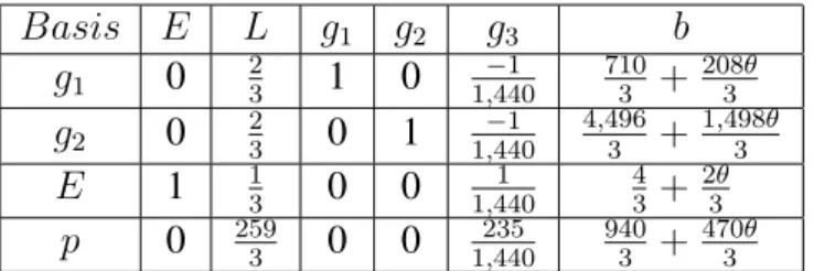
E 3 1 0 0 ₄₈₀1 4 + 2θ C 979 0 0 0 368₄₈₀ 1,472 + 736θ

Table 8: Matrix Multiplication of the Simplex Method and the Tolerance Level

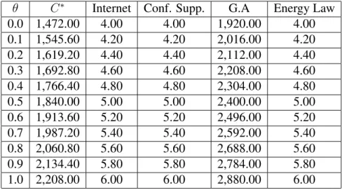
θ C∗ Internet Conf. Supp. G.A Energy Law

0.0 1,472.00 4.00 4.00 1,920.00 4.00

0.1 1,545.60 4.20 4.20 2,016.00 4.20

0.2 1,619.20 4.40 4.40 2,112.00 4.40

0.3 1,692.80 4.60 4.60 2,208.00 4.60

0.4 1,766.40 4.80 4.80 2,304.00 4.80

0.5 1,840.00 5.00 5.00 2,400.00 5.00

0.6 1,913.60 5.20 5.20 2,496.00 5.20

0.7 1,987.20 5.40 5.40 2,592.00 5.40

0.8 2,060.80 5.60 5.60 2,688.00 5.60

0.9 2,134.40 5.80 5.80 2,784.00 5.80

1.0 2,208.00 6.00 6.00 2,880.00 6.00

C∗ = (1,472 + 736θ)N GN

and x∗ = (E∗, L∗) = (0,4 + 2θ). Therefore, the final result for the parametric problem is in Table 9.

From the analysis above on cost minimisation, the Energy Law program viably increases the cost of running the institute.

4.4 Proposed Model

(13)

g1 0 0 1 ₁−_,238₄₆₈ ₁_,90202₀₅₆_,₉₆₀ 0

L 0 1 0 ₁_,₄₆₈3 ₇₀₄−758_,₆₄₀ 1

E 1 0 0 ₁−_,₄₆₈1 ₂_,₁₁₃2,226_,₉₂₀ 1

p 0 0 0 ₁455_,₄₆₈ ₂₃_,1₄₈₈ 1,395₃

each program), then the new linear programming problem becomes:

M ax p(E, L) = 235E+ 230L, (25)

s.t. g1(E, L) = 119E+ 119L≤238 g2(E, L) = 758E+ 742L≤1,500 and

g3(E, L) = 1,440E+ 480L≤1,920,whereEis Energy Studies andLis Energy

Law.

Using the Simplex method, Table 10 was obtained.

The membership functions of the constraints, respectively Internet, con-ference support and Graduate Assistants are:

µ1(E, L) =           

1, ifg1(E, L)≤238

1− g1(E,L)−238

70 , 238< g1(E, L)<308

0, g1(E, L)≥308

(26)

µ2(E, L) =           

1, ifg2(E, L)≤1,500

1−g2(E,L)−1,500

500 , 1,500< g2(E, L)<2,000

0, g2(E, L)≥2,000

(27)

µ3(E, L) =           

1, ifg3(E, L)≤1,920

1−g3(E,L)−1,920

960 , 1,920< g3(E, L)<2,880

0, g3(E, L)≥2,880

(14)

g1 0 0 1 −₁_,230₄₆₈ ₁_,₀₅₆90202_,₉₆₀ 74₁,_,901₀₅₆,_,120₉₆₀θ

L 0 1 0 ₁_,₄₆₈3 ₇₀₄−758_,₆₄₀ 1 - ₁11_,₀₅₆,520_,₉₆₀θ

E 1 0 0 ₁−_,₄₆₈1 ₂_,₁₁₃2,226_,₉₂₀ 1 +₁708_,₀₅₆,480_,₉₆₀θ

p 0 0 0 ₁455_,₄₆₈ ₂₃_,1₄₈₈ 1,395₃ +163₁_,,₀₅₆939_,,₉₆₀200θ

Table 11: Matrix Multiplication of the Simplex Method and the Tolerance Level

Hence,

M ax p= 235E+ 230L, (29)

s.t. g1(E, L) =E+L≤238 + 70(1−α)g2(E, L) = 758E+ 742L≤1,500 +

500(1−α)andg3(E, L) = 1,440E+ 480L≤1,920 + 960(1−α).

Settingθ= 1−α, the following is the parametric problem:

M ax p= 235E+ 230L, (30)

s.t. g1(E, L) = E +L ≤ 238 + 70θ g2(E, L) = 758E + 742L ≤ 1,500 +

500θandg3(E, L) = 1,440E+ 480L≤1,920 + 960θ,

whereθ ∈[0,1]is a parameter.

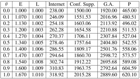
Using the parametric technique and final result of simplex method, Table 11 was obtained. The optimal solution is

p∗ = (1,395 3 +

163,939,200θ

1,056,960 )N GN = 465 + 155.10445N GN

andx∗ = (E∗, L∗) = (1 + ₁708_,₀₅₆,480_,₉₆₀θ,1− ₁11_,₀₅₆,520_,₉₆₀θ ).

Therefore, the final result for the parametric problem is given in Table 12.

From the analysis above, the profit of the institute increased greatly as a result of the viable contribution from both programs.

5 Conclusions

(15)

θ E L Internet Conf. Supp. G.A. P 0.0 1.000 1.000 238.00 1500.00 1920.00 465.00 0.1 1.070 1.001 246.09 1551.53 2016.96 480.51 0.2 1.130 1.002 254.18 1603.06 2113.92 496.02 0.3 1.200 1.003 262.28 1654.58 2210.88 511.53 0.4 1.270 1.004 270.37 1706.11 2307.84 527.04 0.5 1.340 1.005 278.46 1757.64 2404.80 542.55 0.6 1.400 1.006 286.55 1809.17 2501.76 558.06 0.7 1.470 1.007 294.64 1860.70 2598.72 573.57 0.8 1.540 1.008 302.74 1912.22 2695.68 589.08 0.9 1.600 1.009 310.83 1963.75 2792.64 604.59 1.0 1.670 1.010 318.92 2015.28 2889.60 620.10

6 Acknowledgements

The authors acknowledge the support of the members of staff of the Centre for Petroleum Economics, Energy and Law and those of the Water Venture where the data used in this study were obtained.

References

[1] D. Ali, M. Yohanna, M.I. Puwu and B.M. Garkida, Long-term load fore-casting modelling using a fuzzy logic approach, Pacific Science Review A: Natural Science and Engineering 18 (2016), 123–127.

[2] D. Anuradha and V.E. Sobana, A survey on fuzzy transportation problems, IOP Conf. Ser.: Mater. Sci. Eng. 263 (2017) 042105.

[3] R.E. Bellman and L.A. Zadeh, Decision–Making in a Fuzzy Environment, Management Science 17(4) (1970), 141–164.

[4] G.B. Dantzig,Maximization of a linear function of variables subject to lin-ear inequalities, T.C. Koopmans (Ed.): Activity Analysis of Production and Allocation, Cowles Commission Monograph, No. 13, Wiley, New York, (1951), 339–347.

(16)

[6] M. Delgado, J.L. Verdegay and M.A. Vila,A General Model for Fuzzy Lin-ear Programming, Fuzzy Sets and Systems 29 (1989), 21–29.

[7] L.E. Dubins, Finitely additive conditional probabilities, conglomerability, and disintegrations, The Annals of Probability 3 (1995), 88–99.

[8] D. Goldfarb, G.L. Nemhauser and M.J. Todd,Linear Programming, Elsevier Science Publishers B. V., North-Holland 1 (1989).

[9] N. Guzel, Fuzzy Transportation Problem with the Fuzzy Amounts and the Fuzzy Costs, World Applied Science Journal 8(5) (2010), 543–549.

[10] R.E. Hamid, J.A. Mohammad and K. Sahar,Solving a Linear Programming with Fuzzy Constraint and Objective Coefficients, I.J. Intelligent Systems and Applications 7 (2016), 65–72.

[11] S. Hoskova-Mayerova, A. Maturo, Decision-making Process Using Hyper-structures and Fuzzy Structures in Social Sciences. Soft Computing Appli-cations for Group Decision-making and Consensus Modeling. Studies in Fuzziness and Soft Computing, 357 (2017), 103–111. Switzerland: Springer International Publishing AG, ISBN 978-3-319-60206-6.

[12] C.J. Huang, C.E. Lin and C.L. Huang,Fuzzy Aproach For Generator Main-tenance Scheduling, Electric Power Systems Research 24 (1992), 31–38.

[13] J. Kaur and A. Kumar, Mehar’s method for solving fully fuzzy linear pro-gramming problems with L-R fuzzy parameters, Applied Mathematical Mod-elling 37 (2013), 7142–7153.

[14] G.J. Klin and B. Yuan, Fuzzy sets and fuzzy logic theory and applications, Prentice-Hall Inc, New Jersy, 1995.

[15] F.H. Lotfi, T. Allahviranloo, M.J. Alimardani and L. Alizadeh,Solving a full fuzzy linear programming using lexicography method and fuzzy approximate solution, Applied Mathematical Modelling 33(7) (2009), 3151–3156.

[16] C.V. Negoita, Pullback Versus Feedback, Human System Management 1 (1980), 71–76.

[17] C.V. Negoita, The Current Interest in Fuzzy Optimization, Fuzzy Sets and Systems 6 (1981) 261–269.

(17)

[19] H. Tanaka and K. Asai, Fuzzy Linear Programming Problems with Fuzzy Numbers, Fuzzy Sets and Systems 13 (1984), 1–10.

[20] H. Tanaka, T. Okuda and K. Asai, On Fuzzy-Mathematical Programming, Journal of Cybernetics 3(4) (1974), 37-46.

[21] J.L. Verdegay, Fuzzy Mathematical Programming, Fuzzy Information and Decision Process (1982), 231–236.

[22] S.T. Wierzchon, Linear Programming with Fuzzy Sets, Mathl. Modelling 9(6) (1987), 447–459.

[23] L.A. Zadeh,Fuzzy sets, Information and Control 8 (1965), 338-353.

[24] L.A. Zadeh, The Role of Fuzzy Logic in the Management of Uncertainty in Expert Systems, Fuzzy Sets and Systems 11 (1983), 199–227.

[25] H.J. Zimmerman,Description and optimisation of fuzzy system, Int. J. Gen-eral Systems 2 (1976), 209–215.