Optimizing Supply Chain Collaboration Based on Agreement Buyer-Supplier
Relationship with Network Design Problem
Wahyudi Sutopo
1*, Ayu Erliza
2, and Arien Heryansyah
31. Research Group of Logistics and Business System, Department of Industrial Engineering, Universitas Sebelas Maret, Surakarta 57126, Indonesia
2. Department of Industrial Engineering, Universitas Sebelas Maret, Surakarta 57126, Indonesia
3. Centre for Environmental Sustainability & Water Security (IPASA), Universiti Teknologi Malaysia, 81310 UTM Johor Bahru, Malaysia
*e-mail: [email protected]
Abstract
In recent years, the rising competitive environment with shorter product life cycles and high customization forces industries to increase their flexibility, speed up their response, and enhance concurrent engineering designs. To integrate these prospects, supply chain collaboration becomes a pertinent strategy for industries to strengthen their competitiveness. The network design problem is used to implement supply chain collaboration. In the buying and selling process, sharing information between buyer and supplier are important to obtain a transaction decision. The optimimum supply chain profit can be identified by mathematical model of network design problem. The Mathematical Model takes into consideration the uncertainity in negotiation of supply chain, transportation problems, and location-allocation of products from supplier to buyer in the planning based on the time value of money. The results show that the model can be used to optimize the supply chain profit. The supplier gets a profit because income were received in the initial contract, while the buyer profit comes from lower pay.
Abstrak
Optimalisasi Kolaborasi Rantai Pasok berdasarkan Perjanjian Hubungan Pembeli-Pemasok dengan Masalah Desain Jaringan. Pada beberapa tahun terakhir, telah terjadi peningkatan perubahan lingkungan industri, yaitu siklus
hidup produk yang lebih pendek dan adanya dorongan industri harus memeliki kekuatan spesifik agar mampu meningkatkan fleksibilitas, respon pasar, dan meningkatkan kemampuan integrasi desain semua desain proses produk. Untuk mewujudkan peluang ini, kolaborasi rantai suplai menjadi pilihan strategi bagi industri agar dapat memperkuat daya saing mereka. Desain jaringan dapat digunakan pada perbaikan kolaborasi rantai suplai. Dalam proses jual beli, berbagi informasi antara pembeli dan pemasok penting untuk mendapatkan keputusan transaksi. Keuntungan rantai pasokan yang optimum dapat diidentifikasi dengan model matematika dari masalah desain jaringan. Model Matematika yang dikembangkan mempertimbangkan ketidakpastian dalam negosiasi rantai pasokan, masalah transportasi, dan lokasi-alokasi produk dari pemasok kepada pembeli dalam perencanaan dengan mempertimbangkan nilai waktu dari uang. Dari hasil penelitian diketahui bahwa model dapat digunakan untuk mengoptimalkan keuntungan rantai pasokan. Pemasok mendapat keuntungan karena pendapatan yang diterima dalam awal kontrak, sedangkan keuntungan pembeli berasal dari pengeluaran biaya yang lebih rendah.
Keywords: collaboration, negotiation, network design problem, supply chain management, time value of money
1.
Introduction
In recent years, the rising competitive environment with shorter product life cycles and high customization forces industries to increase their flexibility, speed up their their response, and enhance concurrent engineering design [1]. To integrate this, the supply chain collaboration is a good
strategy for the company to strengthen its competitive advantage [1].
location of delivering the products, so, it can minimize the total cost of logistics in the network. Before determining the number and location of delivery, information sharing is required between the buyer and the supplier to obtain the certainty of the transaction prior to the sale process. However, in the implementation, miscommunication often happens between sellers and buyers. Lee et al [2] states that such miscommunication can lead to inefficiencies in utility capacity, shortage/ excess inventory, poor service quality, and others. A number of research have been conducted related to network design problems. One of the earliest works in hub location is by O’Kelly [3] who demonstrated that the one hub location problem is equivalent to the Weber least cost location model.
Shen, Coullard and Daskin [4] illustrate the problem location-inventory problem in which they consider the location of distribution centers to serve a set of retailers, and explicitly describe the implications of inventory location decisions. O’Kelly et al. [5] present exact solutions to hub location models and discussed the sensitivity of these solutions to the inter-hub discount factor used for economies of scale in transportation. Two different hub network designs are considered, single- and multiple-allocation to hubs.
Cheong et al. [6] built the model by including the logistics network design trade-off between stock holding costs and transportation costs at a more detailed level. Stated explicitly in the amount of stock holding cost in the second cycle and safety stock built associated with the different replenishment policy of the supplier to the warehouse.
In addition, several previous studies have conducted research related to supply chain collaboration. Supply Chain Collaboration is defined as two or more companies sharing the responsibility for the planning and management of mutual exchange, implementation and measurement of performance information of such firms [7]. With the existence of this collaboration, there will be coordination between the activities of the companies which work together to produce superior performance and to share the risks and profits.
Zartman [8] states that negotiation is a process of decision-making and participants must be from a number of possible options. However, the final decision does not depend on the negotiators. All negotiators have a mutual influence on decision-making in the supply chain.
Simatupang and Sridharan [9] state that the sharing of information and the use of collaborative methods do not guarantee success. The more partners work together, the more time and money must be spent to ensure proper
collaboration. In addition, the partnership will not continue if one member does not earn enough profit or if one member tries to divert the collaboration in his favor. To avoid such situations, Simatupang and Sridharan [9] realized the need to use incentives such as price agreements or quantity discounts to influence decision actors and to be inclined towards optimization of the global network.
Dudek and Stardler [10] describe a negotiation-based scheme for collaborative planning two-tier SCs consisting of a single supplier and a buyer and extending the negotiation mechanism to cover multiple buyers. The amount of information exchanged between the partners by ordering the buyer to be used as information sharing to offset the rising cost of initial income. Planning decisions such as purchasing, production, transportation, and inventory supplier-buyer to the attention of the mathematical models are constructed.
Habibie et al. [12] state that securing availability of inventory product is needed in the supplier-buyer relationship. Also, in implementing uncertainty to production capacity, demand, and prices, the supply chain will be under sustainability [13].
Previous research about supply chain collaboration based on agreement buyer-supplier relationship has been con-ducted. Rau [14] conducted research related to developing an agent-based negotiation model between buyer and supplier with consideration of multiple deliveries. This article optimized profit between supplier and buyer by the influence of negotiation parameters on negotiation performance.
Hammervoll [15] discusses integrated supply-chain relationships in practice through the utilisation of a new and comprehensive decision-support tool. The article integrates collaborative relationships, enhanced commu-nication and trust between the parties, and substantial savings in distribution costs, achieving mutual benefits from closer collaboration between buyers and suppliers of transportation services that are associated with a transition from arm's-length transactional relationships. The article also generates an application of the decision-support tool for the problem. But, this article does not discuss the bargaining power of suppliers and buyers that can influence distribution costs.
destination, and also the effect of the time value of money incurred in network design for shipping costs. This research will develop the collaboration of network design problem and a model of Chang [1] to accommodate the existing problems in food manufacturing. Food manufacturers established a supply chain collaboration with one of its suppliers using the system contracts. A contract was made containing a pricing deal to buy/sell. The contract states that the selling price should not be set higher than the selling price to a third party. In addition, product purchases should be done collectively to the supplier so that the determination is made after shipping the product to the food manufacturer. The problems related to supply chain collaboration in food manufacturing is when the supplier has not yet determined the number of deliveries made to each destination point which lead to supplier inventory shortages related to its information. In addition, buyers also have trouble knowing the total costs to be incurred after the delivery of the product into their hands. In addition, there is a problem negotiating the price (bargaining power) between the company and the price of competitors that will greatly affect pricing decisions. The mathematical model was built to optimize the supply chain profit by including uncertainty in the negotiations supply chain, transportation problems, and allocation of products from supplier to buyer in the planning, taking into account the time value of money.
2.
Methods
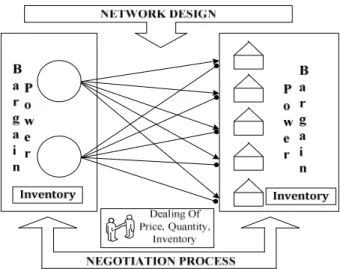
Supply chain collaboration is considered a relevant system for the problem (Figure 1). In this study, the supplier and the buyer have a contract for the sale price. The contract is set by the supplier in which the agreed selling price should not be higher than the selling price to the other third party buyer that sells the same products. Therefore, there will be negotiations for the selling price
Figure 1. Relevant System of the Problem
between the buyer and the supplier. The supplier decides the sale price of the same product per each plant. Total buyer expenses (income supplier) are determined at the point of ordering the product.
In the real system, it is possible for a supplier to have some factories and each plant should send its orders to the destination point. The delivery of products will incur a shipping fee at the amount agreed on in the contract. This is known as network design problems [6]. The supplier does not allocate the amount of products shipped to the buyer destination points early in the planning, so that separate shipping and payment made after the product is handed to the buyer. The time needed to ship the products is 14 days from when the goods are shipped from the warehouse sellers.
This study assumes a real collaboration between partners and the exchange of all information (information sharing). The sharing of information between buyers and suppliers is needed to obtain certainty in the transaction prior to the sale. Sharing this information will be made in a contract system. The basis of a contract system is the negotiation between buyers and suppliers. Real collaboration might not be practical in the supply chain and bargaining power should be implemented to determine the level of a particular company within the negotiation process. Therefore, negotiations will affect the achievement of the objectives of each entity. Constructed mathematical models are used to optimize the supply chain profit collaboration which include uncertainties in the negotiation of supply chain, transportation problems, and allocation of products from supplier to buyer in the planning, taking into account the time value of money.
This research will develop Chang’s model [1] to accommodate the existing problems in food manufacturing.
Table 1. The Definition of Parameter
Notation Definition of parameter
Cs Shipping cost of the supplier
C’s Shipping cost of the supplier in the future time
Dr Demand of buyer
Hr Inventory cost of the buyer
Hs Inventory cost of the supplier
Iro Initial inventory of the buyer
Iso Initial inventory of the supplier
Kr Warehouse capacity of the buyer
Ks Warehouse capacity of the supplier
Pr Purchasing price of the buyer
Psi Selling price of other suppliers (competitor)
Pro Price lower bound of the buyer
Pso Price lower bound of retailer
Qso Manufacturing quantity of supplier with price of
Qro Order quantity of retailer with price of
α Bargaining power
Table 2. The Definition of DecisionVariable
Notation Definition of variable
Pr Purchasing price of the buyer
Ps Selling price of other supplier
Qr Order quantity of buyer
Qs Manufacturing quantity that shipping from
supplier to buyer
Ir Inventory of buyer
Is Inventory of supplier
A formulated mathematical model is constructed using Non-Linear Programming Model. Notations and ex-planations for the parameters and decision variables are described as below.
3.
Result and Discussion
In this case, the supplier and the buyer are involved in the decision-making of the contract to be performed. With different objectives, perhaps sharing information between the supplier and the buyer is the best.
Model for the determinationof supplier’s selling Price. The supplier determines the price for delivering the products to each destination based on the selling price and the shipping cost to any location. The selling price of the supplier is determined on the minimum selling price of the bargaining power supplier in the contract with the quantity of the products delivered and the minimum quantity of sales of products specified by the supplier. There is a limit to the selling price of the supplier where the supplier’s selling price may be greater or equal to the purchase price specified by the buyer. In addition, the selling price is influenced by the selling price of supplier’s competitors. Thus, the selling price of the supplier’s product should not be higher than the purchase price of the buyer to third parties other than those (competitors of the supplier) who sell the same product.
The total of the product selling cost is the sum of the selling price and shipping cost. Because the shipping fee is charged at the beginning, the concept of time value of money is needed so that the supplier and the buyer can estimate the net present from the fees charged to them.
sij s
sij
P
C
P
=
+
for all supplier’s factory from supplier (i) tobuyer (j) (1)α 1 1 1 − = =
Σ
Σ
×
=
so sij n j m i s soQ
Q
P
P
(2)si s r
so
P
P
P
P
≤
≤
≤
(3)(
)
( )
tsij sij
sij
C
Q
r
C
'=
×
×
1
+
− (4)Model for the determination of Buyer’s purchasing price. Buyer’s purchasing price is determined on the minimum purchase price of the buyer bargaining power on contract with the quantity of products received and the minimum purchase quantity of products specified by the buyer. The buyer's purchase price can be greater or equal to the lower limit of the specified buyer purchase price. In addition, the purchase price of the product should not be higher than the purchase price of the buyer from other third parties (competitor of the supplier) who sell the same product.
α 1 1 1 − = =
Σ
Σ
×
=
ro r n j m i r roQ
Q
P
P
(5)si r
ro
P
P
P
≤
≤
(6)
Determination model for inventory of the Supplier. Information about inventory of the supplier is required. The existing inventory amount will affect the holding cost of supplies. Inventory is determined based on the beginning inventory owned by the supplier, the quantity delivered to the buyer, and the demand of the buyer.
mj n j sji n j m i soi m i si m
i=1
I
=
Σ
=1I
+
Σ
=1Σ
=1Q
−
Σ
=1D
Σ
(7)
Determination model for the inventory of the Buyer. As well as the usefulness of the inventory information for the supplier, the inventory information for the buyer is also required. The end of the existing inventory amount will affect the costs incurred by the buyer, in this case, the holding cost. In addition, the inventory information can be used as data to analyze the quantity of the next purchase. Inventory is determined based on the beginning inventory owned by the buyer, the quantity delivered by the supplier, and the demand of the customer. rj n j rji n j m i roi n j rj n
j=1
I
=
Σ
=1I
+
Σ
=1Σ
=1Q
−
Σ
=1D
Σ
(8)
sij n i m i rj n
j=1
D
=
Σ
=1Σ
=1Q
Σ
, for j = 1,…, n (9)
si m i sij n i m
i=1
Σ
=1Q
≤
Σ
=1K
Σ
for i = 1, …, m (10)Buyer’s constraint. In this model, it is assumed that all demands can be met by the supplier. On the other hand, suppliers have the production capacity to meet demand so that there is a capacity constraint buyer to accept orders as requested. The number of products received should be less than or equal to the requested demand.
rij n i m i rj n
j=1
D
≤
Σ
=1Σ
=1Q
Σ
(11)ri m i sij n i m
i=1
Σ
=1Q
≤
Σ
=1K
Σ
(12)The objectives function. The existence of a contract between the supplier-buyer is expected to give a big profit to the supplier. On the other hand, buyers expect a minimum expenditure for each purchase process. The mathematical model of the objective function is denoted by Z1 and supplier to supplier objective function denoted by Z2.
Max Z1=
(
)
si sm i sij sij n
j m
i
Σ
P
×
Q
−
Σ
I
×
H
Σ
=1 =1 =1(13)
Min Z2 :
(
)
rj rn j rij rij n
j m
i
Σ
P
×
Q
+
Σ
I
×
H
Σ
=1 =1 =1(14)
Solution Methods and Analysis. To solve the problems of the food manufacturing, researchers used software LINGO9. Data collection was conducted to obtain data that are used as an input parameter in the calculation of the model built. Preliminary data were used as input parameters of bargaining power value of 0.5 to 1. This shows that for a set price, the supplier and the buyer have the same great bargaining power in the negotiations. Based on the annual report [16], the supplier has 2 factories with a capacity of repectively 9,500 and 5,500 tons per day. The buyer has 14 factories. Therefore, every factory of the supplier can ship orders to all plant buyers. The lower limit of supplier determines the selling price of IDR 5,336,000.00. The lower limit of buyers purchase price was set at IDR 5,500,000.00. The competitor's price is IDR 6.000.000,00. Cost savings are set for suppliers and buyers amounting to respectively IDR 450,000.00 per ton and IDR 540,000.00 per ton. Buyer demand is shown in Table 3 and shipping costs are shown in Table 4.
The result from input parameter and running by LINGO9 Software is shown in the Table 5.
Table 3. Demand per Day
Warehouse Buyer Demand (ton) Warehouse Buyer Demand (ton)
Warehouse B1 800 Warehouse B8 1755
Warehouse B2 850 Warehouse B9 1200
Warehouse B3 900 Warehouse B10 1250
Warehouse B4 950 Warehouse B11 1050
Warehouse B5 875 Warehouse B12 1000
Warehouse B6 900 Warehouse B13 1025
Warehouse B7 1500 Warehouse B14 945
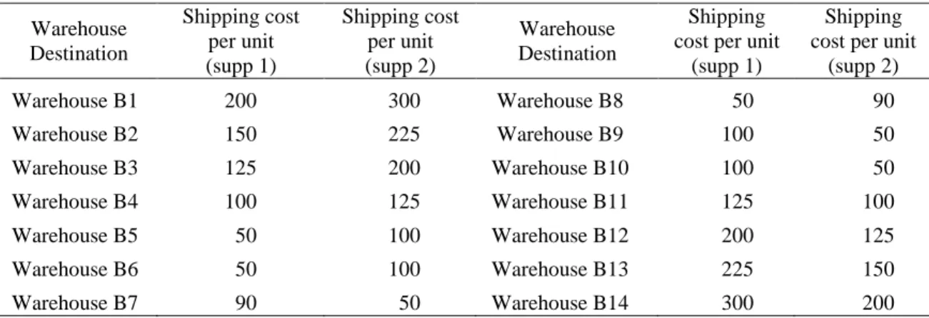
Table 4. Shipping Cost from the Supplier’s Warehouses to Buyer’s Warehouses
Warehouse Destination
Shipping cost per unit (supp 1)
Shipping cost per unit (supp 2)
Warehouse Destination
Shipping cost per unit
(supp 1)
Shipping cost per unit
(supp 2)
Warehouse B1 200 300 Warehouse B8 50 90
Warehouse B2 150 225 Warehouse B9 100 50
Warehouse B3 125 200 Warehouse B10 100 50
Warehouse B4 100 125 Warehouse B11 125 100
Warehouse B5 50 100 Warehouse B12 200 125
Warehouse B6 50 100 Warehouse B13 225 150
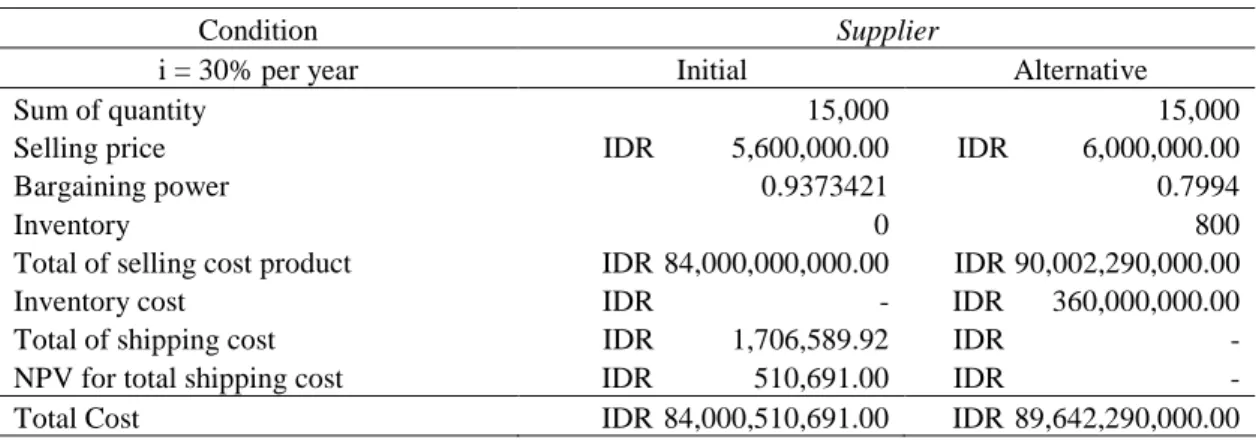
Table 5. Comparison between Initial Model Solution and Alternative Model Solution for Supplier
Condition Supplier
i = 30% per year Initial Alternative
Sum of quantity 15,000 15,000
Selling price IDR 5,600,000.00 IDR 6,000,000.00
Bargaining power 0.9373421 0.7994
Inventory 0 800
Total of selling cost product IDR 84,000,000,000.00 IDR 90,002,290,000.00 Inventory cost IDR - IDR 360,000,000.00 Total of shipping cost IDR 1,706,589.92 IDR - NPV for total shipping cost IDR 510,691.00 IDR -
Total Cost IDR 84,000,510,691.00 IDR 89,642,290,000.00
Table 6. Comparison between Initial Model Solution and Alternative Model Solution for Buyer
Buyer Condition i = 30% per year
Initial Alternative
Sum of quantity 15,000 15,000
Selling price IDR 5,600,000.00 IDR 6,000,000.00
Bargain power 0.9373421 0.7994
Inventory 1500 800
Total of purchasing cost IDR 84,000,000,000.00 IDR 90,002,290,000.00
Inventory cost IDR 975,000,000.00 IDR 520,000,000.00
Total of shipping cost IDR 1,706,589.92 NPV for total shipping cost IDR 510,691.00
Total Cost IDR 84,975,510,691.00 IDR 90,522,290,000.00
The bargaining power of the proposed model has a lower value than the initial model. This shows that with supply chain collaboration there is a decline of power from one of the parties to form the dealing price. This effect on the resulting new price agreement is the rising price of sale/purchase.
In early models, there is the use of NPV (net present value) to convert the value of the total cost of shipping. This happens because the new shipping charges will be paid after the products have been delived to the buyer. In the proposed model, there are no shipping costs because it has accumulated in the cost of product sales at the beginning of the contract agreement. This will be beneficial for the supplier because the supplier receives income in the early contract deal. And also, because it is favorable for buyers to pay less for shipping at the beginning of a deal (the effect of the time value of money).
Verification of model. Verification is done by checking the consistency of the whole unit of mathematical equations in the model. Equation (1)-(6) show the performance criteria which have dimensions of cost
Figure 2. Sensitivity Analysis
(IDR). Equation (7)-(12) show that the performance criteria have a number of product dimensions (units). Meanwhile, the objective function shows that the performance criterion is the result of multiplying the cost and the amount of product (IDR-units)
Changes in cost savings are possible each year depending on the company's stock holding cost policy. Changes in the cost savings will have a direct impact on the amount of inventory that will be the end of the supplier and the buyer obtained. Changes in the cost savings and are divided into two, namely an increase in the cost savings and reduced storage costs with the values set at 10%, 20%, 30%, and 40%.
The chart above shows that the higher the cost savings, the greater the expenditure and revenue decreases. In addition, the graph shows that there are significant changes in supplier revenues and expenditures to the buyer significant cost saving changes.
Based on the numerical example, it can be proved that the model developed is able to cover the limitations of the previous model, in addition we can prove that Model of Rau [14] and Chang [1]. The proposed model can be used to determine the allocation of products to each destination. This model can be used as a consideration in the decision-making SCM for a supplier-buyer relationship that has a contract system. In this system the contents of the contract schedule states the separation between the delivery of goods and the payment of shipping, but the shipping fee is charged at the beginning. Thus, the supplier and the buyer can estimate the present net from the fees charged to them.
4.
Conclusions
This research has been able to build a model that can be used to optimize the supply chain profit by including uncertainties in the negotiation of the supply chain, transportation problems, and allocation of products from supplier to buyer in the planning, taking into account the time value of money. Optimization is carried out on suppliers to gain on income received in early contract deal. Similarly, the buyer makes a profit because of lower pay.
References
[1] Chang, Proceedings of the International Multi Conference of Engineers and Computer Scientists, Hong Kong, Vol. II., 2013.
[2] H.L. Lee, V. Padmanabhan, S. Whang, Manage. Scie., 43 (1997) 558.
[3] M.E. O’Kelly, Transportation Sci, 20 (1986) 106. [4] Z-J.M. Shen, C. Coullard, M.S. Daskin, Transport.
Sci, 37 (2003) 55.
[5] M.E. O’Kelly, D. Bryan, D. Skorin-Kapov, J. Skorin-Kapov, Location Science, 4 (1996) 138. [6] M.L.F. Cheong, R. Bhatnagar, S.C. Graves, J. Ind.
Manage. Optim, 3 (2007) 69.
[7] S. Min, A.S. Roath, P.J. Daugherty, S.E. Genchev, H. Chen, A.D. Arndt, R.G. Richey, Int. J. Logist. Manage,16 (2005) 256.
[8] I.W. Zarman, The 50% Solution, Anchor, New York City, NY, 1976.
[9] T.M. Simatupang, R. Sridharan, Int. J. Logist. Manage,13 (2002) 30.
[10]G. Dudek, H. Stadtler, Int. J. Prod. Res, 45 (2007) 484.
[11]Chopra and Meindl, Handbook of Supply Chain Management, 2nd ed., Pearson Education, United State of America.
[12]A. Habibie, M. Hisjam, W. Sutopo, K.H. Widodo, Proceeding of the Internasional MultiConference of Engineers and Computer Scientists, Hong Kong, 2012.
[13]B. Kurniawan, M. Hisjam, W. Sutopo, IEEE-IEEM, 2011, p.437.
[14]H. Rau, C.-W. Chen, W.-J. Shiang, IEEE International Conference on Networking, Sensing and Control, Japan, 2009, p.312.
[15]T. Hammervoll, E. Bø, Eur. J. Marketing, 44 (2010) 1139.