Integration of Spatial Join Algorithms for Processing
Multiple Inputs
Nikos Mamoulis
Department of Computer Science Hong Kong University of Science and TechnologyClear Water Bay, Hong Kong http://www.cs.ust.hk/~mamoulis/
Dimitris Papadias
Department of Computer Science Hong Kong University of Science and TechnologyClear Water Bay, Hong Kong http://www.cs.ust.hk/~dimitris/
A
BSTRACTSeveral techniques that compute the join between two spatial datasets have been proposed during the last decade. Among these methods, some consider existing indices for the joined inputs, while others treat datasets with no index, providing solutions for the case where at least one input comes as an intermediate result of another database operator. In this paper we analyze previous work on spatial joins and propose a novel algorithm, called slot
index spatial join (SISJ), that efficiently computes the spatial join
between two inputs, only one of which is indexed by an R-tree. Going one step further, we show how SISJ and other spatial join algorithms can be implemented as operators in a database environment that joins more than two spatial datasets. We study the differences between relational and spatial multiway joins, and propose a dynamic programming algorithm that optimizes the execution of complex spatial queries.
Keywords
Spatial Joins, Spatial Query Processing, Query Optimization.
1. I
NTRODUCTIONThe large and steadily increasing availability of multidimensional data in various forms (e.g., satellite images, digital video, multi-media documents) has rendered spatial query processing as one of the most active research areas in the database community. In ad-dition to conventional applications, such as GIS, spatial query processing techniques have been successfully employed in a num-ber of domains including medical information systems and time series databases. Several types of spatial queries have been stud-ied; these include window queries (spatial selections) [Gut84], relation-based queries [PTSE95], nearest neighbors [RKV95] and similarity search [PM98]. Traditional methods used in relational databases are not directly applicable for spatial queries due to the fact that there is no total ordering of objects in space that pre-serves spatial proximity [Gün93]. As a result, a number of spatial
access methods (SAMs) have been proposed [GG98].
The most popular spatial access method is the R-tree [Gut84], which can be thought of as an extension of B+-tree in multi-dimensional space. Each R-tree node consists of a number of
en-tries of the form (MBR, ptr). At leaf node enen-tries, MBR is the minimum bounding rectangle of a data object and ptr is the id of the object. At intermediate node entries, MBR is the minimum bounding rectangle of all data objects under the R-tree node pointed by ptr. Each R-tree node (except from the root) should contain at least a number of entries (minimum R-tree node
utiliza-tion). The R*-tree [BKSS90] is an improved version of R-tree that
employs a sophisticated insertion algorithm, achieving best qual-ity of intermediate nodes. The R-tree and R*-tree are dynamic SAMs that build and maintain their structure incrementally, thus serving as efficient index methods for spatial data. Packing algo-rithms [RL85, KF93, vdBSW97] build optimal R-tree structures from a static set of objects in space. The resulting packed R-trees have full leaf nodes, and thus minimum number of nodes and height, leading to minimization of search time.
Among the most important spatial queries is the spatial join, which retrieves from two datasets all object pairs that satisfy a spatial predicate (e.g., “find all pairs of cities and rivers that
inter-sect”). The first known work on spatial joins is by Orenstein
[Ore86], who proposes a 1-dimensional ordering of spatial objects that uses space-filling curves (z-ordering), and B+-trees to index them. The spatial join is then performed in a merge join fashion, whereas range queries can be answered using the B+-tree index. Rotem [Rot91] describes the creation and maintenance of a spatial join index, analogous to the relational join index, that indexes two spatial relations and is especially used to compute their join. Günther [Gün93] proposes a method that joins two inputs, pro-vided that they are both indexed by generalization trees. A gener-alization tree can be either a spatial access method, or some hier-archical conceptual structure.
Brinkhoff et al. [BKS93] describe an algorithm and some optimi-zation techniques that compute the spatial join of two datasets indexed by R-trees. This method, called R-tree join (RJ), syn-chronously traverses both trees, excluding pairs of nodes that do not intersect, based on the simple observation that such pairs can-not contain overlapping MBRs. RJ is considered as one of the most important spatial join methods, due to its efficiency and the popularity of R-trees. Huang et al. [HJR97a] present a breadth-first search optimized version of RJ that is very efficient when a reasonably large buffer is available. After the RJ algorithm, re-search interest focused on spatial join processing when no index is available for some input.
Suppose that we have to join two inputs; the first is indexed by an R-tree, while the second one is not indexed (e.g., it comes as re-sult of another query operation). Lo and Ravishankar [LR94] propose an algorithm, seeded tree join (STJ), that builds an R-tree-like index (seeded tree) for the second set and then joins the two trees using RJ. The same authors deal with the problem of
Proceedings of the ACM SIGMOD International Conference on Management of Data, Philadelphia, Pennsylvania, June 1999.
joining two sets, none of which is indexed. A hash-join based method (HJ) is presented in [LR96]. HJ uses sampling informa-tion to partiinforma-tion the first dataset, creating a number of buckets which may overlap. The second set is then partitioned into buck-ets with the same extents as the first set’s buckbuck-ets, replicating an object when it overlaps more than one bucket. The spatial join is finally performed by joining the pairs of buckets that have the same extent. These techniques are discussed and analyzed further in section 2.
Patel and DeWitt [PD96] describe another hash-join based algo-rithm, partition based spatial merge join (PBSM), that regularly partitions the space and hashes both inputs into the partitions. It then joins groups of partitions that cover the same area using a plane-sweep technique [PS85] to produce the join results. Some objects from both sets may be assigned in more than one parti-tions, so the algorithm needs to sort the results in order to remove the duplicate pairs. Another algorithm that uses a regular space decomposition is the size separation spatial join (S3J) [KS97]. S3
J avoids replication of objects during the partitioning phase by in-troducing more than one partition layers. Each object is assigned in a single partition, but one partition may be joined with many upper layer partitions. The number of layers is usually small enough for one partition from each layer to fit in memory, thus multiple scans of the files during the join phase are avoided. S3J uses Hilbert curve ordering to sort the partitions inside the layers, and to avoid extra pointers between partitions of different layers. A recent paper [APR+98] proposes an algorithm, called scalable
sweeping-based spatial join (SSSJ), that applies combination of
plane sweep and space partitioning to join the datasets, and works under the assumption that in most cases the “horizon” of the sweep line will fit in main memory. However, the algorithm can-not avoid external sorting of both datasets which may lead to large I/O overhead.
In summary, RJ should be used when both inputs are indexed by R-trees, while there is a variety of good algorithms (HJ, PBSM, S3J and SSSJ) for non-indexed inputs. Currently, however, there does not exist an efficient method for joining two inputs out of which only one is indexed. In section 2, we show that STJ is not always applicable and other methods like indexed nested loop join, and packed R-tree building are, in general, inefficient. In section 3, we propose an algorithm, called Slot Index Spatial Join (SISJ), which is very efficient when only one input is indexed by an R-tree. SISJ is motivated by STJ and HJ, but outperforms both of them analytically and experimentally. Section 4 presents a gen-eral method that computes the multiway join between more than two spatial datasets by combining pairwise join algorithms. The technique applies RJ when both inputs are indexed, SISJ when only one R-tree exists, and HJ if no indexes are present. Query optimization is performed through a dynamic programming algo-rithm using cost models for the pairwise joins and analytical for-mulae for the expected size of intermediate results. Finally, sec-tion 5 concludes the paper with direcsec-tions for future work.
2. B
ACKGROUNDLet A, B be two sets of objects in space out of which only A is indexed by an R-tree RA. Alternative methods that compute the
spatial join between A and B include:
(i) probe each object from B against RA (indexed nested loop
join).
(ii) build an on the fly R-tree index RB for B, and then join RA
and RB using RJ.
(iii) build a seeded R-tree for B, and then join the trees [LR94]. (iv) do not consider the index of the first input, and use a spatial
join algorithm for non-indexed inputs [LR96, PD96, KS97, APR+98].
The indexed nested loop algorithm (i) is a viable choice, only when the size of input B is small enough for the expected number of accesses in RA not to exceed the total number of pages in the
index; in the general case it is too expensive. Patel and DeWitt [PD96] use a bulk loading technique that builds a Hilbert packed R-tree [KF93] for set B, under the assumption that the size of B is smaller than the available buffer. For typical situations (i.e., the size of B is greater than the buffer), however, method (ii) is ex-pensive because of the large overhead of external sorting prior to building RB. [LR94] shows that method (iii) outperforms (ii) by a
wide margin but it does not consider bulk loading in the imple-mentation of (ii). In [LR96], it is suggested that method (iv) using HJ, can be more efficient than approaches that use indices. In the sequel we describe in detail STJ and HJ.
2.1 Seeded tree join
The seeded tree method [LR94] joins two spatial inputs, provided that only one is supported by an R-tree. This technique builds a second R-tree using RA as a seed, and then applies RJ to join the
two R-trees. The motivation behind creating a seeded R-tree for the second input, instead of a normal R-tree, is the fact that a seeded tree with extents similar to RA nodes will be more efficient
during tree matching, as the number of overlapping node pairs between the trees will be smaller. Thus, the seeded tree construc-tion algorithm creates an R-tree that is optimal for spatial join and not for range searching.
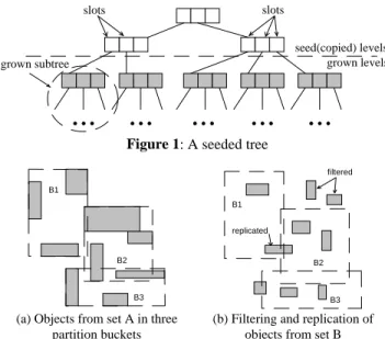
The seeded tree construction is divided in two phases: the seeding and the growing phase. In the seeding phase the top k levels (k is a parameter of the algorithm) of RA are copied to formulate the top
k levels of the seeded tree SB. The entries of the lowest level of SB
are called slots. After copying, the slots maintain the copied ex-tent, but they point to empty (null) sub-trees. During the growing phase, all objects from B are inserted into SB. A rectangle is
in-serted under the slot that contains it, or needs the least area en-largement. Figure 1 shows an example of a seeded tree structure. The top 2 levels of the R-tree are copied to guide the insertion of the second dataset.
Lo and Ravishankar propose some techniques that optimize the structure of the seeded tree, and a filtering mechanism that rejects rectangles from the second set that do not overlap any of the seed slots. They also present a tree construction technique that reduces I/O page accesses when the size of the tree exceeds the size of the available memory buffer. If this happens, many pages may have to be fetched and written back to disk during a single insertion, re-sulting in a large I/O cost. In order to avoid buffer thrashing, the objects which are to be inserted under a slot are written in a tem-porary file. After all objects are inserted, an R-tree is constructed for each temporary file, and is pointed by the corresponding slot in the seeded tree. To implement this mechanism and minimize random I/O accesses, at least one page is allocated in the buffer for each slot. If the buffer is full, all slots that have more than a constant number of pages flush their data to disk and memory is freed.
A problem with STJ, however, is that it cannot be applied in every case. In order for the above algorithm to work efficiently, the number of slots S should not exceed the number of pages M in the system buffer. If S≥M, it is not possible to avoid buffer thrashing,
which may lead to a large I/O penalty. Thus the algorithm is inef-ficient when the fanout of the R-tree nodes is large and the mem-ory buffer is relatively small. Consider, for instance, a dataset of 100,000 objects which are indexed by a 8K page size R-tree (a rather typical case). Under the assumption that each node entry is 20 bytes long (16 for the x- and y-coordinates, plus 4 for the ob-ject id or block reference), the capacity of a tree node is 409; thus the dataset can be indexed by a 2-level R-tree, with 245 leaf nodes and 1 root. When trying to apply STJ, we have to copy the root level of the R-tree to the seeded tree, which results in S=245. As a consequence the algorithm cannot be applied for buffers smaller than 1.96Mbytes.
2.2 Spatial Hash-Join
Spatial hash-join (HJ) [LR96], based on the relational hash-join paradigm, computes the spatial join of two inputs, none of which is indexed. Set A is partitioned into S buckets, where S is decided using the system parameters. The initial extents of the buckets are determined by sampling. Each object is inserted into the bucket that is enlarged the least. Set B is hashed into buckets with the same extent as A’s buckets, but with a different insertion policy; an object is inserted into all buckets that intersect it. Thus, some objects may go into more than one bucket (replication), and some may not be inserted at all (filtering). The algorithm does not en-sure equal sized1 partitions for A, as sampling cannot guarantee the best possible slots. Equal sized partitions for B cannot be guaranteed in any case, as the distribution of the objects in the two datasets may be totally different. Figure 2 shows an example of two datasets, partitioned using the HJ algorithm.
After hashing set B, the two bucket sets are joined; each bucket from A is matched with only one bucket from B, thus requiring a single scan of both files, unless for some pair of buckets none of them fits in memory. If one bucket fits in memory, it is loaded and the objects of the other bucket are prompted against it. If none of the buckets fits in memory, an R-tree is built for one of them, and the bucket-to-bucket join is executed in an indexed nested-loop fashion.
Experiments in [LR96] show that HJ is better in terms of I/O than building two seeded trees and joining them. It is also shown that this algorithm is faster than spatial join with pre-computed R-tree indices (RJ), if the difference between sequential and random disk accesses is taken into account. We believe that this comparison of HJ with RJ is unfair. First, as we show in section 3, RJ is signifi-cantly faster than HJ in terms of CPU-time. Second, as shown in [KC98], when a R-tree packing method that places sibling nodes in sequence is used, the I/O performance of RJ in terms of I/O is significantly improved. In the rest of the paper, we will not con-sider the difference between random and sequential I/O accesses. We cannot draw conclusive results about the relative performance of HJ with respect to other algorithms that perform joins of non-indexed inputs (i.e., PBSM, S3J, SSSJ). The experiments in [KS97] suggest that S3J behaves best when the datasets contain
1
The term "size of partition/slot" denotes the number of objects inside the partition, and not its spatial extent.
relatively large rectangles and extensive replication occurs in HJ and PBSM. HJ is, in general, expected to perform better than PBSM, because the latter requires sorting of the results in order to remove duplicate solutions. In [APR+98] SSSJ is compared only with PBSM, and was found inferior in the average case (but better for skewed data). Furthermore, SSSJ requires sorting of both data-sets to be joined, and therefore it does not favor pipelining and parallelism of spatial joins. On the other hand, the fact that PBSM uses partitions with fixed extents makes it suitable for processing multiple joins in parallel [PYK+97].
3. T
HES
LOTI
NDEXS
PATIALJ
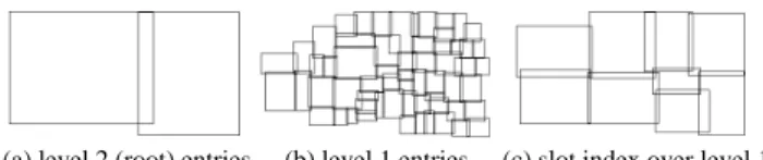
OINAs shown in section 2, STJ is not always applicable due to buffer size limitations. In this section we propose a novel algorithm, called slot index spatial join (SISJ), which is very efficient when only one R-tree index exists, and can be used independently of the buffer size. The motivation behind SISJ is to apply hash-join, using as buckets the entries of the topmost R-tree level that leads to a desired number of partitions S. In order to overcome the limitation of buffer size, (i.e., when the number of entries is larger than the buffer size M), SISJ groups the entries of the selected tree level to S (possibly overlapping) partitions called slots. Each slot contains the MBR of the indexed R-tree entries, along with a list of pointers to these entries. The algorithm uses the MBRs of the slots to hash set B. Hash-join is then performed by joining each bucket of set B with the data under the R-tree entries pointed by the corresponding slot in the slot index. Figure 3 illustrates a 3-level R-tree (the leaf 3-level is not shown) and a slot index built over it. If M=10, the root level contains too few entries to be used as partition buckets. As the number of entries in the next level are over M, we have to partition them in S=9 (for this example) slots (notice that STJ cannot be applied in this case).
As stated before, S should be smaller than M in order to avoid buffer thrashing. The lower limit of S is such that the expected number of data from set A in each slot will fit in memory. If PA is
the number of pages that can fit the first dataset (i.e. the number of RA leaf nodes assuming that RA is packed), then:
seed(copied) levels grown levels slots slots
...
...
...
...
...
grown subtreeFigure 1: A seeded tree
B1 B2 B3 B1 B2 B3 filtered replicated
(a) Objects from set A in three partition buckets
(b) Filtering and replication of objects from set B
M S M < < PA (1)
in order for the data under each slot to fit in memory. There exist some cases (when M is very small compared to PA) that the lower
limit PA/M should be ignored. Consider, for instance, that the
page size is 8K, the buffer size is 128K, and set A consists of 100,000 objects (=2Mbytes); then M=128/8=16 and PA = 245. Eq.
(1) results in 16 < S < 16, which does not provide a valid value for
S. Thus, the lower limit is ignored and the partitions are not
guar-anteed to fit in memory. More details about the choice of S are given in section 3.3.
3.1 The SISJ algorithm
SISJ takes as parameter the desired number of slots S according to eq. (1). The topmost tree level k with total number of entries nE >
PA/M is the level where partitioning will take place 2
. If nE is
within the valid range for S, i.e. PA/M < nE < M, S is exactly nE
and the slots will have as extents the MBRs of these entries. If nE ≥ M, we cannot directly use the entries nE to partition and the slot
index should be built. A good partitioning mechanism will mini-mize total area and overlap between the slots, and will evenly distribute the entries. We consider 3 policies of partitioning the nE
entries into S groups:
(i) SplitXL: sort entry MBRs with respect to their lower
x-coordinate and divide them into S equal sized groups. This method is motivated by [RL85].
(ii) SplitHC: sort entry MBRs with respect to the Hilbert value
of their center and divide them into S equal sized groups. SplitHC is motivated by [KF93].
(iii) IRS: insert the entries into S slots using the R*-tree insertion
algorithm [BKSS90].
From the above partitioning methods, SplitXL and SplitHC in-clude just sorting and splitting. The third partitioning method, IRS (insert, re-insert and split), is more sophisticated. Starting from a single empty slot, for each entry e, the following insertion algo-rithm is called:
Algorithm IRS(RTreeEntry e)
1. choose a slot s, such that e.MBR is contained into s.MBR.
1a. If more than one such slots exist, choose the one with the smallest area.
1b. If no such slot exists, choose the one that causes the minimum overlap enlargement (between the slots) when e is inserted to it. 2. insert e into s and update its MBR.
2a. If s overflows, and no other overflow has occurred during this in-sertion:
• sort the entries in s according to their distance of their centers to
the center of s.MBR
• delete from s the 30% last (furthest) entries and update s.MBR
• re-insert the entries into the slots
2b. If s overflows, and overflow has reoccurred during this insertion:
• apply the R*-tree split algorithm to split s into 2 slots.
The first part of IRS is equivalent to the ChooseSubtree R*-tree algorithm that determines the best leaf node when inserting a rec-tangle. Part 2a is equivalent to the Forced Reinsert, whereas 2b is
2
Under typical system conditions (e.g. page size 4K-8K, M=64) usually k will be the root level, or the level under the root.
the R*-tree split algorithm. IRS does not guarantee slots of equal size; the equal size splitting criterion is not considered in order to favor the good shape criterion. To ensure that the final number of partitions after IRS will be “around S”, and considering that the slot utilization is 70% on the average [BKSS90] (given that slots will be at least 40% full), we set as slot capacity (10/7)⋅(nE/S), so
that the average number of entries in a slot will be nE/S. The final
number of buckets may not be S but will definitely be between 70%S (if all buckets are full) and (7/4)⋅S (if all buckets are 40%
full). If these limits are out of the valid range, the maximum slot capacity should be tuned correspondingly. Notice that the ex-pected nE cannot exceed min(M⋅CA, CA2), where CA is the node
capacity (maximum fanout) in RA, otherwise the upper tree level
should be used for partition. Therefore, all three partitioning poli-cies can take place in main memory with trivial CPU time cost. In section 3.3 we empirically compare these three splitting policies. After building the slot index, the second set B is hashed into buckets with the same extents as the slots. As in HJ, if an object from B does not intersect any bucket it is filtered; if it intersects more than one buckets it is replicated. The join phase of SISJ is also similar to the corresponding phase of HJ. All data from RA
indexed by a slot are loaded and joined with the corresponding hash-bucket for set B. When the buffer does not permit the R-tree data under a slot to fit in memory, it may be natural for the parti-tions of the second set not to fit in memory, as well. If these sets are small, external sorting + plane sweep [APR+98] or indexed nested loop join (using as root of the R-tree the corresponding slot), may work well, but for large sets the best solution is the recursive application of SISJ, in a similar way to recursive hash-join [SKS97]. During the hash-join phase of SISJ, when no data from B is inserted into a bucket, the R-tree data under the corresponding slot do not need to be loaded (slot filtering).
3.2 Analysis of SISJ
In this section we provide formulae for the cost of SISJ in terms of I/O, and analytically compare the algorithm with STJ and HJ. Let A be the first dataset, which is indexed by an R-tree RA, and B
the second dataset, for which no index exists. TA denotes the
number of pages (blocks) of RA, and PB is the number of pages of
B. Initially, the slots have to be determined from A. This requires loading the top k levels of RA in order to find the appropriate slot
level. Let sA be the fraction of RA nodes from the root until k. The
slot index is built in memory, thus no additional I/O is required. Set B is then hashed into the slots requiring PB accesses for
read-ing, and PB + rBPB - fBPB accesses for writing, where rB is the
fraction of replicated data and fB is the fraction of filtered data.
Thus, the cost of SISJ partition phase is:
Cpart = sA⋅TA + (2+rB-fB)⋅PB (2)
Next, the algorithm will join the contents of the buckets from both sets. If for each joined pair at least one bucket fits in memory, then a single scan is required; the smaller partition is loaded in memory and each object of the other partition is probed against it. If no bucket fits in memory, pages may have to be fetched more
(a) level 2 (root) entries (b) level 1 entries (c) slot index over level 1
than once from the disk. We consider the typical case, where the buffer is large enough, for at least one partition to fit in memory. For fairness, we make the same assumption when analyzing STJ and HJ. The pages from set A that have to be fetched for the join phase are the remaining (1-sA)⋅TA, since the pointers to the slot
entries are kept in the slot index and need not be loaded again from the top levels of the R-tree. Moreover, some of these will not be fetched at all, if a slot is filtered. We consider the worst case and ignore the possibility of filtered slots for dataset A. The num-ber of I/O accesses required for the join phase is:
Cjoin = (1-sA)⋅TA + (1+rB-fB)⋅PB (3)
considering that the join output is not written back to disk. Sum-marizing, the total cost of SISJ is:
CSISJ = Cpart + Cjoin = TA + (3+2rB-2fB)⋅PB (4)
The cost of HJ (under the same assumptions as SISJ) is:
CHJ = Csampling + 3PA + (3+2rB-2fB)⋅PB (5)
in accordance with the corresponding formula in [KS97]. HJ re-quires Csampling random accesses to determine the initial slots and
an extra reading and writing to hash A. After hashing A and de-termining the final bucket extents, HJ follows the same procedure with SISJ. From eq. (4) and (5), and given that for typical R*-tree structures PA = 70%TA, SISJ clearly outperforms HJ in terms of
I/O.
Next, we provide an analysis of the seeded tree join (STJ). We charge the same I/O for copying the seed levels, as for determin-ing the slots in SISJ, i.e. sATA. For fairness to STJ, we assume that
a grown sub-tree can fit in memory. Thus the growing phase costs 3PB + TB because the second set has to be initially read and
writ-ten under the slots in sequential files; then the sequential files have to be read to build the grown sub-trees, and finally, TB tree
pages have to be written back (as the whole seeded tree is not expected to fit in memory). The join phase for STJ is expected to cost at least TA + TB (all pages from both trees are read during RJ
[HJR97b]). Summarizing,
CSTJ = (1+sA)⋅TA + 3PB + 2TB (6)
From eq. (4), (6) we can conclude that the cost difference between STJ and SISJ is: CSTJ - CSISJ = sATA+ 2TB - (2rB - 2fB)⋅PB. For
reasonable filtering and replication ratios, the difference is sub-stantial; STJ needs an extra read/write for the seeded tree (2TB)
which is a considerable overhead. Furthermore, STJ is expected to be more expensive than SISJ in terms of CPU-time, due to the CPU-intensive seeded tree construction. In conclusion, SISJ re-tains (i) the advantage of STJ, which avoids partitioning the first set using information from the R-tree to decide the hash-bucket extents and (ii) the advantage of HJ, which avoids on-the-fly R-tree building, requiring to read the second set only twice.
3.3 Experimental evaluation of SISJ
In order to evaluate the performance of SISJ we conducted three sets of experiments. We first compare the quality of the three par-titioning policies (SplitXL, SplitHC and IRS), then we test the effect of S in the performance of SISJ, and finally, SISJ is com-pared with HJ and RJ. In our experiments we used several real and synthetic data files, described in Table 1. Files AS, AL, AU, and AH are publicly available at http://www.maproom.psu.edu/dcw/. T1 and T2 [Bur89] are commonly used to benchmark spatial join algorithms [BKS93, LR96, HJR97a, KC98]. The synthetic files G1 and G2 were created according to a Gaussian distribution with 16 clusters. The centers of the clusters were randomly generated, and the sigma value of the data distribution around the clusters followed a random value between 1/20 and 1/10 of the map size. The density of a dataset is defined as the total area of the rectan-gles divided by the area of the workspace3. An R*-tree was built for each dataset. The page size (equal to the tree node size) was set to 8K, and the buffer size was set to 512K. Table 1 also shows the height h of the corresponding R*-trees, the number P of pages that fit the datasets in a sequential file and the number T of tree nodes. All experiments were run on an UltraSparc2 workstation (200 MHz) with 256MB of main memory.
Set Description size density h P T
GS Greek roads 23268 0.33 2 57 88 GR Greek rivers 24650 0.39 2 61 93 AS German roads 30674 0.08 2 75 113 AL German railroads 36334 0.07 2 89 129 AU German utilities 17790 0.12 2 44 69 AH German hypsography 76999 0.04 2 189 276 T1 California roads 131461 0.05 3 322 469 T2 California rivers+railroads 128971 0.39 3 316 428 U1 Uniform distributed MBRs 100000 0.5 2 245 324 U2 Uniform distributed MBRs 100000 1 2 245 321 G1 Gaussian distributed MBRs 100000 0.5 2 245 328 G2 Gaussian distributed MBRs 100000 1 2 245 329
Table 1: Characteristics of the datasets used at the experiments First, we test the quality of the three partitioning policies of SISJ. Figure 4(b) shows the set of 466 level 1 entries of the T1 R*-tree (the root contains just two entries). If we set S = 20, and follow policies SplitXL, SplitHC, and IRS, we get the partitions of Fig-ure 4(c), 4(d) and 4(e), respectively. The figFig-ures show that IRS achieves better quality partitions (smaller overlap and total area) than SplitXL and SplitHC. Figure 5 presents the effect of the three
3
Given a series of different layers of the same region (e.g. rivers, streets, forests), its workspace is defined as the total area cov-ered by all layers (not necessarily rectangular) including holes, if any.
(a) California roads (T1) (b) Leaf node MBRs of T1 (c) SplitXL partitioning (d) SplitHC partitioning (e) IRS partitioning
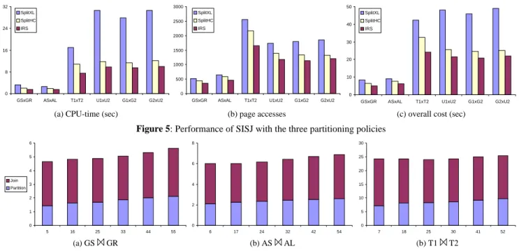
policies on the performance of SISJ for various join pairs. The overall time was computed after charging 10ms for each page access, a typical value for modern disks [SKS97]. In all cases IRS is substantially better than the other two policies, with SplitXL performing very bad because of the extensive replication it intro-duces. The inferior performance of SplitXL and SplitHC is due to the fact that the entries to be split have large spatial extents [vdBSW97]. In the rest of the paper we adopt IRS as the standard SISJ partitioning policy.
In the next experiment we test the effect of S on the performance of SISJ. The overall cost of the three joins that involve real data-sets is split to partitioning and join cost (Figure 6). Notice that there is no significant difference in performance for the different choices. The partitioning time grows slightly with S, as more bucket extents have to be tested and more replication is intro-duced. The join time is larger for small S when the datasets are large (e.g., T1 T2), because the chance that some buckets for a hash partition will not fit in memory increases. As the differences are trivial, a relatively large S, which will certainly lead to parti-tions that fit in memory, is a safe choice.
In the final set of experiments, we compare SISJ with HJ and RJ. The number of slots S in the experiments was set to 25 for both HJ and SISJ. When SISJ was applied, the R-tree index for the first set was used. Most pairs of buckets to be joined fitted in memory and a fast plane sweep technique was utilized to perform the join. For RJ, the page replacement policy in the buffer was LRU. Fig-ure 7 illustrates the performance of all three algorithms. Because STJ cannot be applied in the current experimental setting without buffer thrashing (nE>M), we omit it from the evaluation.
From the charts we can conclude that SISJ is clearly the best choice when only one index exists; it outperforms HJ in all cases. RJ is the clear winner, if R-trees exist for both sets, a fact that was expected. The CPU overhead of HJ in comparison to RJ is large, thus, even if the difference between random and sequential I/O is considered, RJ still outperforms HJ. In some cases (e.g. GS GR, AS AL), the CPU-time overhead of HJ is very large. We
ob-served that in these cases HJ spends most of its time partitioning the first dataset; if an object is not contained in any slot, the ap-propriate slot has to be determined and updated based on some factors (overlap, area) that are CPU-intensive. When the first da-taset is clustered, the above situation is very common and the time to partition the first set is considerable. In order to test the parti-tioning overhead in HJ and SISJ, we decomposed the processing of the first three joins into partition and join time for all algo-rithms (Figure 8). Observe that HJ, SISJ and RJ require almost the same time at join phase. This indicates that as long as partitions of good quality have been constructed, the time to join them is close to the optimal. The performance gap between HJ and SISJ is mainly due to the difference between partitioning the first dataset (for HJ) and constructing the slot index (for SISJ). The construc-tion of the slot index never exceeded 1% of the total CPU-time. In summary, SISJ is a spatial hash join algorithm that achieves very good performance when computing joins in the presence of a single R-tree, based on the following properties:
• The hash-buckets are decided upon the tree structure and no
extra I/O for hashing the build input is needed.
• The partitions of the build input are guaranteed to have,
ap-proximately, the same number of objects, as they point to almost the same number of R-tree entries. Thus, skewed data are han-dled very efficiently.
In the rest of the paper we show how SISJ can be combined with other spatial join algorithms to process complex spatial queries involving multiple inputs.
4. P
ROCESSING OFM
ULTIWAYS
PATIALJ
OINS In spatial database applications the user is not limited to simple selections and joins, but queries often involve processing of nu-merous spatial sets, or combinations of spatial and non-spatial attributes. Here, we deal with the problem of joining more than two spatial inputs in a uni-processor, centralized environment. As an example consider the query “find all cities that intersect a river which also passes through an industrial area”. Such queriesre-0 8 16 24 32
GSxGR ASxAL T1xT2 U1xU2 G1xG2 G2xU2 SplitXL SplitHC IRS 0 500 1000 1500 2000 2500 3000
GSxGR ASxAL T1xT2 U1xU2 G1xG2 G2xU2 SplitXL SplitHC IRS 0 10 20 30 40 50
GSxGR ASxAL T1xT2 U1xU2 G1xG2 G2xU2 SplitXL
SplitHC IRS
(a) CPU-time (sec) (b) page accesses (c) overall cost (sec)
Figure 5: Performance of SISJ with the three partitioning policies
0 1 2 3 4 5 6 5 16 25 33 44 55 Join Partition 0 2 4 6 8 6 17 24 32 42 54 0 5 10 15 20 25 30 7 18 25 30 41 52 (a) GS GR (b) AS AL (b) T1 T2
quire (i) determining a good execution plan that will minimize the evaluation time and usage of resources, and (ii) an execution en-gine that applies this plan, by effectively managing the synchroni-zation between the spatial join operators.
Multiway spatial joins can be expressed by a query graph Q(V,E), where each node V corresponds to a spatial relation, and each edge E to a join predicate. Figure 9(a) shows the graph of a mul-tiway join that involves four relations. The query can be processed by applying several combinations of pairwise join algorithms. For instance, the plan in Figure 9(c) may involve the execution of RJ for determining R3 R4. The intermediate result may then be
joined with R2 (using SISJ), and finally with R1. On the other
hand, the plan of 9(d) corresponds to executing R1 R2 and
R3 R4 using RJ, and joining the intermediate results using HJ.
In this section we provide cost models and optimization tech-niques for the processing of multiway spatial joins.
R1 R2 R3 R4 R1 R2 R3 R4 R1 R2 R3 R4 R1 R2 R3 R4
(a) query graph (b) left-deep plan (c) right-deep plan (d) bushy plan
Figure 9: a query and some alternative ways of processing
4.1 Special issues about multiway spatial joins
Many techniques that deal with the optimization and execution of complex relational queries in centralized and distributed environ-ments have been proposed during the last 20 years (see [Gra93] and [JK84] for two surveys). Early query optimization methods considered only left-deep plans, because the first join algorithms (nested loops and merge join) made other plans either impossible, or very expensive. Furthermore, they did not allow for concurrent execution of multiple joins. For instance, merge join calls for writing and sorting of intermediate results, thus pipelining and
concurrent execution of many joins is not possible unless the in-termediate results are sorted on the next join’s attribute (an un-common situation). Left-deep plans are linear in nature and re-strict the space of possible execution orders, making the optimi-zation procedure faster. Later, the development of hash-join algo-rithms shifted attention towards bushy and right-deep plans. The trade-off is the explosion of the query optimization search space; the excessive number of execution plans makes query optimiza-tion a time-consuming task, and several hill-climbing techniques that discover sub-optimal plans in reasonable time have been pro-posed (e.g., [IK90]).
The techniques available for relational joins, however, are not readily applicable to multiway spatial joins. The main difference between relational and spatial queries is the non-transitivity of the most common spatial predicate overlap, as opposed to the transi-tivity of the equal (=) predicate in relational natural and equi-joins. As a result, the following apply for multiway spatial joins:
• Cycles cannot be eliminated in the same way as in the relational
model. Cycle elimination in relational queries is based on the transitivity of the equal predicate [BC81]. For instance, consider three relations R1, R2, R3 and the cycle ((R1.A = R2.B), (R2.B =
R3.C) and (R1.A = R3.C)). As the third clause is implied by the
first two, it can be safely ignored. On the other hand, if A,B,C are spatial relations and the predicate is overlap instead of equal, the third clause is not inferred from the first two and, therefore, it cannot be removed.
• • •
• The number of possible execution plans does not explode as fast
as in relational joins. For instance, the relational query ((R1.A =
R2.B) and (R2.B = R3.C)), can be executed using the plan
(R1 R3) R2, which is not valid for the corresponding spatial
query ((R1 overlap R2) and (R2 overlap R3)). The total number of
plans when joining n spatial inputs depends on the form of the query graph. Complete graphs (cliques) may lead to a number of join plans comparable to the corresponding number for relational queries, but in general, queries are simpler (i.e., with fewer edges
0 2 4 6 8 10 12 14
GSxGR ASxAL T1xT2 U1xU2 G1xG2 G2xU2 HJ SISJ RJ 0 500 1000 1500 2000 2500
GSxGR ASxAL T1xT2 U1xU2 G1xG2 G2xU2 HJ SISJ RJ 0 5 10 15 20 25 30 35
GSxGR ASxAL T1xT2 U1xU2 G1xG2 G2xU2 HJ
SISJ RJ
(a) CPU-time (sec) (b) page accesses (c) overall cost (sec)
Figure 7: Performance of HJ, SISJ and RJ
0 4 8 12 16 HJ SISJ RJ Join Partition 0 4 8 12 16 HJ SISJ RJ Join Partition 0 5 10 15 20 25 30 35 HJ SISJ RJ Join Partition (a) GS GR (b) AS AL (b) T1 T2
than complete graphs). Moreover, joining a large number of spa-tial inputs (e.g., >10) is uncommon, as opposed to relational que-ries which have a broader number of applications. Thus, exhaus-tive search in the whole space of possible plans is feasible.
4.2 Execution of multiway spatial joins
Following the relational query processing paradigm, multiway spatial joins can be processed by implementing a set of join op-erators. The algorithm used for a spatial join operator depends on whether an index exists for the underlying inputs. Thus, RJ can be applied only when the inputs are leaves in the execution plan, i.e., datasets indexed by R-trees. SISJ is employed when only one input is indexed by an R-tree. Because of the symmetry of RJ and SISJ, we only consider right-deep plans, where the left input is indexed by an R-tree (each left-deep plan can be transformed to an equivalent right-deep plan). In all other cases (i.e., bushy plans), a spatial join algorithm which joins inputs with no index is used. For simplicity, we employ HJ due to its common modules with SISJ, even though other algorithms (e.g., PBSM, S3J and SSSJ) could also be applied.
Multiway joins with cycles can be executed by transforming them to tree expressions using the most selective edges of the graph and filtering the results with respect to the other relations in memory. For instance, consider the cycle (R1 overlap R2), (R2 overlap R3),
(R3 overlap R1) and the query execution plan R1 (R2 R3).
When joining the tuples of (R2 R3) with R1 we can use either
the predicate (edge) (R2 overlap R1), or (R3 overlap R1) as the join
condition. If (R2 overlap R1) is the most selective one (i.e., results
in the minimum cost), it is applied for the join and the qualifying tuples are filtered with respect to (R3 overlap R1).
Table 2 shows the iterator functions [Gra93] for all three spatial join algorithms in an execution engine running on a centralized, uni-processor environment that applies pipelining. Since RJ is employed for the leaves, it just executes the join and passes the results to the upper operator. SISJ first constructs the slot index, then hashes the results of the probe (right) input into the corre-sponding buckets and finally executes the join passing the results to the upper operator. HJ does not have knowledge about the ini-tial buckets where the results of the left join will be hashed; thus, it cannot avoid writing the results of its left input to disk. At the same time it performs sampling to determine the initial extents of the hash buckets. Then the results from the intermediate file are read and hashed to the buckets. The results of the probe input are immediately hashed to buckets.
Notice that in this implementation, the system buffer is shared between at most two operators. Next functions never run concur-rently; when join is executed at one operator, only hashing is
performed at the upper operator. Thus, given a memory buffer of
M pages, the operator which is currently performing join uses M-S
pages and the upper operator, which performs hashing, uses S pages, where S is the number of slots/buckets. In this way, the utilization of the memory buffer is maximized.
4.3 Plan cost estimation
In order to determine the optimal plan for a multiway spatial join, we need accurate formulae for estimating the costs of the join operators and the size and distribution of intermediate results. For SISJ and HJ we use the cost formulae given in section 3.2. The cost of RJ is difficult to estimate due to the implication of the LRU buffer. Theodoridis et al. [TSS98] provide an analytical formula that predicts the cost of RJ in terms of node accesses, based on the properties (density, cardinality) of the joined data-sets. In their analysis, no buffer, or a trivial buffer scheme is as-sumed. In practice, however, the existence of a buffer affects the number of page accesses significantly. Here we adopt the formula provided in [HJR97b], which predicts actual page accesses in the presence of an LRU buffer:
CRJ = TA + TB + (NA(RA, RB) - TA - TB)⋅P(node, M) (7)
where NA(RA, RB) is the total number of R-tree nodes accessed by
RJ, and P(node, M) is the probability that a requested R-tree node will not be in the buffer (of size M) and will result in a page fault. More details about the computation of NA(RA, RB) and P(node,
M) can be found in [HRJ97b].
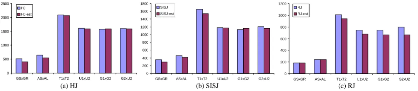
We tested the accuracy of eq. (4), (5) and (7) by calculating esti-mated and actual I/O costs for the join pairs of Figure 7 using the same experimental settings. When estimating the cost of HJ and SISJ (eq (4) and (5)), we set fB = 0 and rB = 20% (typical ratios
for good hash buckets). Figure 10 illustrates the differences be-tween the estimated and experimental values. The formulae for HJ and SISJ are very precise (usually below 10% relative error). The cost formula for RJ is also accurate and, since the joined files cover the same area, the error is between 10% and 20% (in accor-dance with the corresponding experiments in [HJR97b]). There-fore, the analytical cost formulae for HJ, SISJ and RJ are precise enough for inclusion in spatial query optimizers4.
In addition to the join cost, a query optimizer for multiway spatial joins needs formulae for the expected size (i.e., number of
4
The original formulas are slightly modified to capture pipelin-ing; in particular, for HJ and SISJ, we exclude the cost of read-ing the right input, and charge one extra write for the left input of HJ, because it must be materialized.
Iterator Open Next Close
RJ open tree files return next tuple close tree files SISJ (assuming that left
input is the R-tree input)
open left tree file; construct slot index; open right (probe) input; call next on right input and hash results into slots; close right input
perform hash-join and return next tuple
close tree file; deallo-cate slot index and hash buckets HJ (assuming that left input
is the build input and right input the probe input)
open left input; call next on left and write the
results into intermediate file while determining the extents of the hash buckets; close left input; hash all results from intermediate file into left buckets; open right input; call next on right and hash all results into right buckets; close right input
perform hash-join and return next tuple
deallocate hash buckets
tions) of a join, in order to estimate the input size of upper joins. The size of a join output is determined by the following:
• The size of the sets to be joined. If SizeA and SizeB are the sizes
of the inputs, the join may produce up to SizeA⋅SizeB tuples
(Cartesian product).
• The density of the sets. Datasets with large density have
rectan-gles with larger average area, thus producing larger number of intersections.
• The distribution of the rectangles inside the sets. This is the most
difficult factor to estimate, as in many cases the distribution is not known, and even if known, its characteristics are very diffi-cult to capture.
Following the analysis in [TSS98] and [HJR97b], the number of output tuples when joining two datasets A and B with uniform distribution is:
SizeA B = SizeB⋅SizeA⋅(rectA + rectB)2 (8)
where rectA is the average side length of a rectangle in A, and the
rectangle co-ordinates are normalized to take values from [0,1). In other words, the size of A B is the number of rectangles in A intersected by an average rectangle in B, multiplied by the number of rectangles in B. Given the density DA of set A, the average side
length of a rectangle in A is:
rectA = DA/SizeA (9)
When joining files with non-uniform distributions, eq. (8) is not expected to provide an accurate join size estimation. Motivated by an idea from [TSS98], we use statistical information for the distri-bution of the datasets in order to estimate the join size. In par-ticular, we partition the workspace into a grid of equal sized cells. The criterion for assigning a rectangle to a cell is the enclosure of the rectangle’s center, thus no rectangle is assigned to more than one cells. For each cell, the number of rectangles and the normal-ized average rectangle size is kept. The estimation of the join output size is then done using eq. (8) for each cell and summing up the results.
Table 3 shows the estimated join sizes for various grids and the average relative error, where relative error is defined as |estimated
I/O-actual I/O|/actual I/O. For joins involving highly skewed data
(i.e. GS GR) the accuracy of the join size grows with the size of the grid, whereas in other cases even a small grid provides a good prediction. The size of the grid is however crucial for the applica-bility of the method. Since the grid is used to compute the size of intermediate join results during query optimization, it should be small enough to fit in main memory. In our implementation we chose a 50×50 grid because it provides reasonable precision with-out introducing significant overhead.
Pair GS GR AS AL T1 T2 U1 U2 G1 G2 G2 U2 error size 51617 20518 86094 292080 281689 401416 Size estimation No grid 34392 10050 94084 302051 302051 408000 0.17 20×20 31521 11483 69475 302013 289090 412816 0.18 50×50 38495 13154 78312 302801 291332 413522 0.13 100×100 45253 15539 83706 305267 291587 414979 0.08
Table 3: Join output size estimation using grids
In order to compute the output size of a join which takes interme-diate results as input, we may apply eq. (8) for each pair of cells, but now Size corresponds to the number of estimated intermediate results in a cell, and rect is the average rectangle size in the cell of the corresponding joined relation. Consider, for instance, the multiway join ((R1 overlap R2) and (R2 overlap R3)), and the
exe-cution plan R1 (R2 R3): SizeB in eq. (8) becomes SizeR2 R3,
and rectB = rectR2.
Although eq. (8) is accurate for pairwise joins and acyclic multi-way joins, if the query graph contains cycles, it only provides an upper bound for the size of the output. Analytical formulae that estimate the output size of multiway spatial joins with tree and clique graphs are provided in [PMT99]. These formulae can be used in our case to estimate the intermediate results of query sub-graphs that can be decomposed to trees and cliques. For instance, all decompositions of a query that involves four inputs in a cycle are tree subgraphs, thus (8) can be used to estimate their output size.
4.4
Query Optimization
In this section we show how the above analytical formulae can be incorporated in a dynamic programming algorithm that generates the optimal execution plan for multiway spatial joins. Even though the proposed optimal_plan algorithm can be applied for the general case where spatial relations may not be indexed, for simplicity of the pseudo-code we assume that all datasets are in-dexed by R-trees.
The optimal plan for a query is determined in a bottom-up fashion from its subgraphs. Initially, the cost and output size of each pairwise join (i.e., each graph edge) is computed, using equations (7) and (8), respectively. At step i, for each connected subgraph Qi
with i nodes, optimal_plan determines the best decomposition of Qi to two connected parts, based on the optimal cost of executing
these parts and their size. When one of the parts consists of a sin-gle node, SISJ is considered as the join execution algorithm, whereas if both parts have at least two nodes, HJ is used. The output size is estimated using the size of the plans that formulate the decomposition. 0 500 1000 1500 2000 2500
GSxGR ASxAL T1xT2 U1xU2 G1xG2 G2xU2 HJ HJ-est 0 200 400 600 800 1000 1200 1400 1600 1800
GSxGR ASxAL T1xT2 U1xU2 G1xG2 G2xU2 SISJ SISJ-est 0 200 400 600 800 1000 1200
GSxGR ASxAL T1xT2 U1xU2 G1xG2 G2xU2 RJ
RJ-est
(a) HJ (b) SISJ (c) RJ
At the end of the algorithm, Q.plan will be the optimal plan, and
Q.cost and Q.size will hold its expected cost and size. Due to the
bottom-up computation of the optimal plans, the cost and size for a specific query subgraph is computed only once. The price to pay is the storage requirements for the algorithm, which is manageable for typical query graphs. The worst case of time and space re-quirements, is when the graph is complete (clique). Then at level
i, the number of subgraphs to be tested is C(i,n) and the total
stor-age cost is:
C-spaceoptimal_plan() =
∑
= n i i n 2 < 2n (10)Initially, optimal_plan will compute the costs of all pairwise joins (C(2,n) for clique topology). Then at each level i, 2<i≤n, all com-binations C(i,n) of connected subgraphs must be decomposed in order to find the optimal decomposition. Thus, the worst case time requirement for the algorithm is:
C-timeoptimal_plan() =
∑
= ⋅ + n i WC i i n n 3 ) ( ions decomposit # 2 (11)where the (worst case) number of possible decompositions at i is:
#decompositionsWC(i) =
∑
∑
− = − = 1 2 / 1 2 / even is if , 2 -odd is if , i i j i i j i i/ i j i i j i (12)For a clique query with 10 variables, eq. (10) results in 1013, and eq. (11) gives 24,070, which implies that optimization is very fast compared to query execution time. In practice, query graphs usu-ally contain fewer edges (than cliques) and the actual numbers are much smaller than the above bounds. Among acyclic queries with 10 variables, the one that generates the largest number of sub-graphs (=511) has a star topology, while the one that generates the smallest number (=45) has a chain topology. When cost and
size are estimated using a grid, this grid should be maintained and updated for each connected subgraph. Typical queries of n≤10 are able to support a 50×50 grid, given a reasonably large memory buffer.
4.5 Experimental evaluation
We tested the accuracy of the cost formulae and the optimization algorithm for several types of queries. We used the datasets pre-sented in section 3, and created some extra synthetic sets, in order to produce a variety of queries with reasonable output size5. Data-sets U3, U4 (G3, G4) were generated in the same way as U1, U2 (G1, G2) but contain 50,000 rectangles, of density 0.1 and 0.5, respectively. All datasets were indexed by R*-trees with the same parameters as in section 3. The buffer size was set to 512K. We did not consider non-connected query graphs since they can be processed by computing the results of each connected subgraph and then their Cartesian product.
In the experiments we ran 30 queries that involved 3 to 7 syn-thetic datasets, and several queries with the four Germany layers. We applied both cyclic and acyclic queries including chains (e.g., “find all supermarkets which are next to a bank, which is next to a government building”) and star queries (e.g., “find all cities
crossed by a river which also crosses some industrial area and
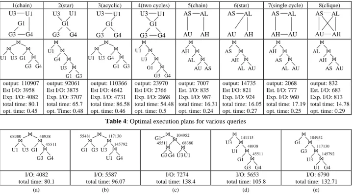
some forest”). The difference between estimated and experimental cost never exceeded 15%, showing that the cost estimation, which is a crucial factor for query optimization, is very accurate. In gen-eral, the average prediction error grew with the number of joined inputs due to accumulation of errors in the estimation of interme-diate join results. For queries involving synthetic sets the estima-tion was very precise, because they are less skewed than real ones. Table 4 illustrates some example queries, and their optimal exe-cution plan, as calculated by optimal_plan using a 50×50 statistics grid. The output size of the queries, the estimated and experi-mental I/O cost, the (actual) overall cost (I/O cost + CPU time) in seconds and query optimization time are provided. Notice that optimization never exceeded 2% of the total cost (usually it ranged between 0.5% and 1%). All right deep plans were proven I/O bound, whereas for some bushy plans the CPU-cost was found comparable to the I/O cost (e.g. query 1). This is due to the HJ algorithm which in some cases is CPU-bound (e.g., see GS GR in Figure 7). In general, bushy plans (that use HJ) were preferred to right-deep plans (where SISJ is applied), only when the number of intermediate results that have to be hashed in slots created by SISJ is very large and their materialization introduces significant I/O overhead. Table 5 illustrates the above observation by pre-senting the execution costs (I/O and overall time) of some plans of the 1st query.
In this query, right-deep plans perform worse than the optimal bushy plan due to the large size of intermediate results before the last (SISJ) join. For instance, plan 5(d) is more expensive than 5(a), because the intermediate result G3 G4 G1 U1 is large. Considering the significant cost difference between alterna-tive plans, optimization may achieve large performance gains while adding minimal overhead. In the optimal plan 5(a), al-though U1 U3 produces more tuples than G3 G4 G1, it is
5
Synthetic datasets U2 and G2 produced an excessive number (in the order of millions) of output tuples when included with U1 and G1 in multiway joins.
Algorithm optimal_plan(Query Q, int n) /*n = number of inputs*/ For Each connected subgraph Q2∈ Q of size 2 Do
Q2.cost = CRJ(A, B); /*eq. (7)*/
Q2.size = Size(A, B); /*eq. (8)*/
EndFor /* Q2 */
For i=3 to n Do
For Each connected subgraph Qi∈ Q with i nodes Do
/*Find optimal plan for Qi*/
Qi.cost = ∞; Qi.plan = NULL;
For Each decomposition Qi→ {Qk, Qi-k}, Qk, Qi-k connected Do
If (k=1) Then /*Qk is a single node; SISJ will be used*/
{Qk, Qi-k}.cost=Qi-k.cost+CSISJ(Qk, Qi-k); /*eq. (4)*/
Else /*both components are sub-plans; HJ will be used*/
{Qk, Qi-k}.cost=Qk.cost+Qi-k.cost+CHJ(Qk, Qi-k); /*eq.(5)*/
EndIf /*k=1*/
If {Qk,Qi-k}.cost<Qi.cost Then /*better than former optimal*/
Qi.plan={Qk, Qi-k}; /*mark decomp. as Qi’s optimal plan*/
Qi.cost={Qk, Qi-k}.cost; /*mark so far optimal cost of Qi*/
EndIf /*mincost*/ EndFor /*decomposition*/
/*Estimate Qi’s output size from optimal decomposition*/
Qi.size = Size(Qi.plan);
EndFor /*Qi*/
EndFor /*i*/ End /*optimal_plan*/
used as the build input (left), because the tuples have smaller length and, as a result, actual size of the materialized results is smaller. Notice that if a semi-join was required (the intermediate results were projected to a single column), G3 G4 G1 could be the build input.
In order to test the accuracy of optimal_plan, we executed all alternative plans for 20 of the tested queries. The algorithm found the best plan in 18 cases. Whenever there was a better plan than the generated one, the difference between the actual optimal and the estimated plan was trivial, and it was due to size estimation errors of intermediate results.
We also tested the effects of the statistical grid in the optimization process. The cost and the optimal plan was estimated for various grid sizes (No grid, 20×20, 50×50, 100×100). As expected, the existence of the grid was of little importance for queries with synthetic datasets. When real datasets were involved the differ-ence was large, due to data skew and different area covered, with the largest grids (50×50, 100×100) achieving more accurate cost and size predictions. In some queries with many inputs and multi-ple join conditions, the 100×100 grid for all possible subgraphs, could not fit in main memory, rendering optimization inapplica-ble. On the other hand, with the 50×50 grid the optimization process was successful for all tested queries.
5. C
ONCLUSIONSThe goal of this paper is to provide an integrated approach to processing pairwise and multiway spatial joins. First, we describe and analyze previous work on spatial join algorithms, with and without indexes on the input relations. Second, we propose a novel spatial join algorithm, slot index spatial join, for the case where only one of the two inputs is indexed by an R-tree. SISJ achieves very good performance because (i) it avoids the expen-sive building of an on-the-fly R-tree, (ii) determines the
hash-bucket extents from the R-tree structure, without hashing the build input, and (iii) it guarantees partitions of equal size for the build input, which, for typical buffers, fit in memory, and thus handles skewed data very efficiently.
Finally, we demonstrate how SISJ and other join algorithms can be implemented as modules of a query execution engine that uses pipelining to process multiple spatial inputs. In addition to ana-lytical formulae that accurately predict the cost of execution plans, we provide a dynamic programming algorithm that determines the optimal plan of multiway spatial joins. The precision of the cost formulae and query optimization is confirmed through extensive experiments with synthetic and real data.
SISJ can be applied for relational joins, provided that the build input is indexed by a B+-tree. The entries of a high B+-tree level are split into S partitions, and the hash-function for the probe input is decided upon the bounds of these partitions. It is not clear whether this method is faster than sorting the probe input and applying merge-sort. A straightforward advantage of SISJ in com-parison to merge-sort approaches, is when the probe input is an output of an underlying database operator and merge-sort requires materialization of the probe input prior to sorting.
Currently, we study the combination of pairwise join algorithms with a generalization of RJ, that synchronously traverses more than two R-trees [PMD98]. Some results [MP99] show that in many cases this method is superior to cascading executions of pairwise join algorithms. We are also interested in investigating the inter-parallelism between spatial join operators. So far, PBSM has been parallelized in Paradise project [PYK+
97], while intra-parallelism of RJ has been shown in [BKS96]. In addition, we plan to test the applicability of relational query decomposition methods (e.g. [BC81]) for spatial query processing.
1(chain) 2(star) 3(acyclic) 4(two cycles) 5(chain) 6(star) 7(single cycle) 8(clique) U3 G1 U1 G3 G4 U3 G1 U1 G3 G4 U3 G1 U1 G3 G4 U3 G1 U1 G3 G4 AS AL AU AH AS AL AU AH AS AL AH AU AS AL AU AH U1 U3 G1 G3 G4 U3 G1 G3 G4 U1 U1 U3 G4 G1 G3 G3 G4 U1 G1 U3 AL AU AS AH AH AL AU AS AS AL AU AH AH AS AU AL output: 110907 Est I/O: 3958 Exp. I/O: 4082 total time: 80.1 opt. time: 0.45 output: 92061 Est I/O: 3875 Exp. I/O: 3707 total time: 65.7 opt. Time: 0.48 output: 110366 Est I/O: 4642 Exp. I/O: 4731 total time: 86.58 opt. time: 0.46 output: 23970 Est I/O: 2766 Exp. I/O: 2868 total time: 54.48 opt. time: 0.5 output: 7007 Est. I/O: 835 Exp. I/O: 987 total time: 16.31 opt. time: 0.24 output: 14735 Est I/O: 821 Exp. I/O: 924 total time: 16.05 opt. time: 0.27 output: 2068 Est. I/O: 777 Exp. I/O: 960 total time: 17.19 opt. time: 0.25 output: 832 Est. I/O: 683 Exp. I/O: 813 total time: 14.78 opt. time: 0.29
Table 4: Optimal execution plans for various queries
U1 U3 G1 G3 G4 68380 48938 45511 G1 G3 U3 U1 G4 55481 117130 145792 G3 G4 U3 U1 G1 68380 104952 45511 G3 G4 U3 G1 U1 141115 48938 45511 U1 G4 G1 U3 G3 104952 117130 145792 I/O: 4082 total time: 80.1 I/O: 5587 total time: 96.07 I/O: 7274 total time: 138.4 I/O: 5653 total time: 105.8 I/O: 6790 total time: 132.71 (a) (b) (c) (d) (e)
A
CKNOWLEDGEMENTThe authors were supported by grant HKUST 6151/98E from Hong Kong RGC and grant DAG97/98.EG02. We would like to thank the Greek Ministry for the Environment, Urban Planning & Public Works for providing us with the GS and GR datasets.
R
EFERENCES[APR+98] Arge, L., Procopiuc, O., Ramaswamy, S., Suel, T., Vitter, J.S. “Scalable Sweeping-Based Spatial Join”.
VLDB, 1998.
[BC81] Bernstein, P.A., Chiu, D.M.W. “Using semi-joins to solve relational queries”. Journal of ACM, vol 28, no 1, pp. 25-40, 1981.
[BKSS90] Beckmann, N., Kriegel, H.P. Schneider, R., Seeger, B. “The R*-tree: an Efficient and Robust Access Method for Points and Rectangles”. ACM SIGMOD, 1990. [BKS93] Brinkhoff, T., Kriegel, H.P., Seeger B. “Efficient
Processing of Spatial Joins Using R-trees”. ACM
SIGMOD, 1993.
[BKS96] Brinkhoff, T., Kriegel, H.P., Seeger, B. "Parallel Processing of Spatial Joins Using R-trees". IEEE
ICDE, 1996.
[Bur89] Bureau of the Census. Tiger/Line Precensus Files:
1990 technical documentation, Washington, DC,
1989.
[Gra93] Graefe, G. “Query Evaluation Techniques for Large Databases”. ACM Computing Surveys, vol. 25, no. 2, pp. 73-170, 1993.
[Gün93] Günther, O. “Efficient Computation of Spatial Joins”.
IEEE ICDE, 1993.
[Gut84] Guttman, A. “R-trees: A Dynamic Index Structure for Spatial Searching”. ACM SIGMOD, 1984.
[GG98] Gaede, V., Günther, O. “Multidimensional Access Methods”. ACM Computing Surveys, vol. 30, no. 2, pp. 123-169, 1998.
[HJR97a] Huang, Y.W., Jing, N., Rundensteiner, E.A. “Spatial Joins using R-trees: Breadth First Travesral with Global Optimizations”. VLDB, 1997.
[HJR97b] Huang, Y.W., Jing N., Rundensteiner, E.A. “A Cost Model for Estimating the Performance of Spatial Joins Using R-trees”, International Conference on
Scien-tific and Statistical Database Management (SSDBM),
1997.
[IK90] Ioannidis, Y., Kang, Y. “Randomized Algorithms for Optimizing Large Join Queries”. ACM SIGMOD, 1990
[JK84] Jarke, M., Koch, J. “Query Optimization in Database Systems”. ACM Computing Surveys, vol. 16, no. 2, pp. 111-152, 1984.
[KC98] Kim, K., Cha S.K., “Sibling Clustering of Tree-based Spatial Indexes for Efficient Spatial Query Process-ing”. ACM CIKM, 1998.
[KF93] Kamel, I., Faloutsos, C. “On Packing R-trees”. ACM
CIKM, 1993.
[KS97] Koudas, N., Sevcik, K. “Size Separation Spatial Join”.
ACM SIGMOD, 1997.
[LR94] Lo, M.L., Ravishankar, C.V. “Spatial Joins Using Seeded Trees”. ACM SIGMOD, 1994.
[LR96] Lo, M.L., Ravishankar, C.V. “Spatial Hash-Joins”.
ACM SIGMOD, 1996.
[MP99] Mamoulis N., Papadias, D. “Synchronous R-tree Tra-versal”. Technical Report, HKUST-CS99-03, 1999. [Ore86] Orenstein, J.A. “Spatial Query Processing in an
Ob-ject-Oriented Database System”. ACM SIGMOD, 1986.
[PD96] Patel, J.M., DeWitt D.J., “Partition Based Spatial-Merge Join”. ACM SIGMOD, 1996.
[PM98] Papadopoulos, A., Manolopoulos, Y. “Similarity Query Processing Using Disk Arrays”. ACM
SIG-MOD, 1998.
[PMD98] Papadias, D., Mamoulis, N., Delis, V., “Querying by Spatial Structure”. VLDB, 1998.
[PMT99] Papadias, D., Mamoulis, N., Theodoridis, Y., “Processing and Optimization of Multi-way Spatial Joins Using R-trees”. ACM PODS, 1999.
[PS85] Preparata, F, Shamos, M. Computational Geometry, Springer, 1985.
[PTSE95] Papadias, D., Theodoridis, Y., Sellis, T., Egenhofer, M. “Topological Relations in the World of Minimum Bounding Rectangles: a Study with R-trees”. ACM
SIGMOD, 1995.
[PYK+97] Patel, J., Yu, J., Kabra, N., et al. “Building a Scalable Geo-Spatial DBMS: Technology, Implementation, and Evaluation”. ACM SIGMOD, 1997
[Rot91] Rotem, D. “Spatial Join Indices”. IEEE ICDE, 1991. [RKV95] Roussopoulos, N., Kelley, F., Vincent, F. “Nearest
Neighbor Queries”. ACM SIGMOD, 1995
[RL85] Roussopoulos, N., Leifker .D. “Direct Spatial Search on Pictorial Databases Using Packed R-Trees”. ACM
SIGMOD, 1985
[SKS97] Silberschatz, A., Korth, H.F., Sudarshan, S. Database
System Concepts. McGraw-Hill, 1997.
[TSS98] Theodoridis, Y., Stefanakis, E., Sellis, T. “Cost Mod-els for Join Queries in Spatial Databases”. IEEE
ICDE, 1998.
[vdBSW97]van der Bercken J., Seeger, B., Widmayer, P. “A Ge-neric Approach to Bulk Loading Multidimensional Index Structures”. VLDB, 1997.

![Table 2 shows the iterator functions [Gra93] for all three spatial join algorithms in an execution engine running on a centralized, uni-processor environment that applies pipelining](https://thumb-us.123doks.com/thumbv2/123dok_us/9244775.2410997/8.918.119.797.113.294/iterator-functions-algorithms-execution-centralized-processor-environment-pipelining.webp)