Image Super-resolution
Lyndsey C. Pickup
Robotics Research Group
Department of Engineering Science
University of Oxford
Michaelmas Term, 2007
Machine Learning in Multi-frame
Image Super-resolution
Abstract
Multi-frame image super-resolution is a procedure which takes several noisy low-resolution images of the same scene, acquired under different conditions, and pro-cesses them together to synthesize one or more high-qualitysuper-resolutionimages, with higher spatial frequency, and less noise and image blur than any of the original images. The inputs can take the form of medical images, surveillance footage, digital video, satellite terrain imagery, or images from many other sources.
This thesis focuses on Bayesian methods for multi-frame super-resolution, which use a prior distribution over the super-resolution image. The goal is to produce outputs which are as accurate as possible, and this is achieved through three novel super-resolution schemes presented in this thesis.
Previous approaches obtained the super-resolution estimate by first computing and fixing the imaging parameters (such as image registration), and then computing the super-resolution image with this registration. In the first of the approaches taken here, superior results are obtained by optimizing over both the registrations and image pixels, creating a complete simultaneousalgorithm. Additionally, parameters for the prior distribution are learnt automatically from data, rather than being set by trial and error.
In the second approach, uncertainty in the values of the imaging parameters is dealt with by marginalization. In a previous Bayesian image super-resolution approach, the marginalization was over the super-resolution image, necessitating the use of an unfavorable image prior. By integrating over the imaging parameters rather than the image, the novel method presented here allows for more realistic prior distributions, and also reduces the dimension of the integral considerably, removing the main computational bottleneck of the other algorithm.
Finally, a domain-specific image prior, based upon patches sampled from other images, is presented. For certain types of super-resolution problems where it is applicable, this sample-based prior gives a significant improvement in the super-resolution image quality.
I owe a lot of thanks to lots of people. . .
Steve Roberts took me on as an undergrad, and I’d like to thank him for helping me become a researcher, and for all his support in making me better at it.
I’d like to thank Andrew Zisserman for making Computer Vision so awesome all along. He pointed me towards super-resolution when I’d lost my way, and I’m indebted to him for all the time and advice he has offered me ever since.
I’m very grateful to my examiners, Andrew Blake and Amos Storkey, for their constructive observations and discussion of my work; my thesis is much stronger now as a result.
I’d like to thank my parents for taking care of me when I’ve had a hard time, for letting me go my own way, and for making it possible for me to pursue what I enjoy.
Last (but never least!) I’d like to thank all my friends for keeping me happy and sane! Particular thanks must go to the wonderful members of OUSFG and
Taruithorn (the Oxford University Speculative Fiction Group and the Oxford Tolkien Society), and also to the lovely people on my LiveJournal “flist” and elsewhere on-line, for updating me on the real world once in a while.
This work was funded by a three-year studentship from the Engineering and Physical Sciences Research Council (EPSRC).
1 Introduction 1
1.1 How is super-resolution possible? . . . 3
1.2 Challenges . . . 4
1.3 Thesis contributions . . . 6
2 Literature review 10 2.1 Early super-resolution methods . . . 11
2.1.1 Frequency domain methods . . . 12
2.1.2 The emergence of spatial domain methods . . . 13
2.1.3 Developing spatial-domain approaches . . . 15
2.2 Projection onto convex sets . . . 16
2.3 Methods of solution . . . 18
2.4 Maximum a posteriori approaches . . . 19
2.4.1 The rise of MAP super-resolution . . . 20
2.4.2 Non-Gaussian image priors . . . 21
2.4.3 Full posterior distributions . . . 25
2.6 Determination of the point-spread function . . . 29
2.6.1 Extensions of the simple blur model . . . 31
2.7 Single-image methods . . . 32
2.8 Super-resolution of video sequences . . . 35
2.9 Colour in super-resolution . . . 36
2.10 Image sampling and texture synthesis . . . 38
3 The anatomy of super-resolution 40 3.1 The generative model . . . 41
3.2 Considerations in the forward model . . . 42
3.2.1 Motion models . . . 43
3.2.2 The point-spread function . . . 44
3.2.3 Constructing W(k) . . . 45
3.2.4 Related approaches . . . 48
3.3 A probabilistic setting . . . 49
3.3.1 The Maximum Likelihood solution . . . 50
3.3.2 The Maximum a Posteriori solution . . . 53
3.4 Selected priors used in MAP super-resolution . . . 59
3.4.1 GMRF image priors . . . 59
3.4.2 Image priors with heavier tails . . . 64
3.5 Where super-resolution algorithms go wrong . . . 69
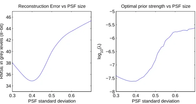
3.5.1 Point-spread function example . . . 69
3.5.2 Photometric registration example . . . 72
3.5.3 Geometric registration example . . . 74
3.6 Super-resolution so far . . . 84
4 The simultaneous approach 86 4.1 Super-resolution with registration . . . 87
4.1.1 The optimization . . . 89
4.2 Learning prior strength parameters from data . . . 90
4.2.1 Gradient descent on α and ν . . . 92
4.3 Considerations and algorithm details . . . 93
4.3.1 Convergence criteria and thresholds . . . 94
4.3.2 Scaling the parameters . . . 94
4.3.3 Boundary handling in the super-resolution image . . . 95
4.3.4 Initialization . . . 97
4.4 Evaluation on synthetic data . . . 100
4.4.1 Measuring image error with registration freedom . . . 100
4.4.2 Registration example . . . 103
4.4.3 Cross-validation example . . . 106
4.5 Tests on real data . . . 109
4.5.1 Surrey library sequence . . . 109
4.5.2 Eye-test card sequence . . . 111
4.5.3 Camera “9” sequence . . . 113
4.5.4 “Lola” sequences . . . 115
4.6 Conclusions . . . 115
5 Integrating over the imaging parameters 119 5.1 Bayesian marginalization . . . 120
5.1.2 Marginalizing over the super-resolution image . . . 126
5.1.3 Implementation notes . . . 128
5.2 Results . . . 130
5.2.1 Butterfly sequence . . . 130
5.2.2 Synthetic eyechart sequence . . . 134
5.2.3 Face sequence . . . 135
5.2.4 Real data . . . 141
5.3 Discussion . . . 142
5.4 Conclusion . . . 145
6 Texture-based image priors for super-resolution 148 6.1 Background and theory . . . 149
6.1.1 Image patch details . . . 153
6.1.2 Optimization details . . . 155
6.2 Experiments . . . 156
6.2.1 Synthetic data . . . 156
6.2.2 Results . . . 158
6.3 Discussion and further considerations . . . 159
7 Conclusions and future research directions 166 7.1 Research contributions . . . 166
7.2 Where super-resolution algorithms go next . . . 168
7.2.1 More on non-parametric image priors . . . 168
7.2.2 Registration models and occlusion . . . 169
7.2.3 Learning the blur . . . 170
7.3 Closing remarks . . . 174
A Marginalizing over the imaging parameters 176 A.1 Differentiating the objective functionw.r.t. x. . . 177
A.2 Numerical approximations forg and H . . . 183
B Marginalization over the super-resolution image 187 B.1 Basic derivation . . . 188
B.1.1 The objective function . . . 188
B.1.2 The Gaussian distribution over y . . . 192
B.2 Gradient w.r.t. the registration parameters . . . 194
B.2.1 Gradients w.r.t. µand Σ. . . 194
Introduction
This thesis addresses the problem of image super-resolution, which is the process by which one or more low-resolution images are processed together to create an image (or set of images) with a higher spatial resolution.
Multi-frame image super-resolution refers to the particular case where multiple images of the scene are available. In general, changes in these low-resolution images caused by camera or scene motion, camera zoom, focus and blur mean that we can recover extra data to allow us to reconstruct an output image at a resolution above the limits of the original camera or other imaging device, as shown in Figure 1.1. This means that the super-resolved output image can capture more of the original scene’s details than any one of the input images was able to record.
Problems motivating super-resolution arise in a number of imaging fields, such as satellite surveillance pictures and remote monitoring (Figure 1.2), where the size of the CCD array used for imaging may introduce physical limitations on the resolution of the image data. Medical diagnosis may be made more easily or more accuratly if
Figure 1.1: Multi-frame image super-resolution. The low-resolution frames to the left are processed together and used to create a high-resolution view of the text, seen to the right. Notice that the bottom row of the eyechart letters cannot be read in any of the input images, but is clear in the super-resolved image.
data from a number of scans can be combined into a single more detailed image. A clear, high-quality image of a region of interest in a video sequence may be useful for facial recognition algorithms, car number plate identification, or for producing a “print-quality” picture for the press (Figure 1.3).
Figure 1.2: An example of super-resolution for surveillance: several frames such as the low-resolution one shown left can be combined into an output frame (right) where the level of ground detail is significantly increased. Images from [102].
Figure 1.3: An example of super-resolution in the media: frame-grabs such as the one of the left can be combined to give a much clearer print-quality image, as on the right. Images from [43].
1.1
How is super-resolution possible?
Reconstruction-based super-resolution is possible because each low-resolution image we have contains pixels that represent subtly different functions of the original scene, due to sub-pixel registration differences or blur differences. We can model these differences, and then treat super-resolution as an inverse problem where we need to reverse the blur and decimation.
Each low-resolution pixel can be treated as the integral of the high-resolution image over a particular blur function, assuming the pixel locations in the high-resolution frame are known, along with the point-spread function that describes how the blur behaves. Since pixels are discrete, this integral in the high-resolution frame is modelled as a weighted sum of high-resolution pixel values, with the point-spreaad function(PSF) kernel providing the weights. This image generation process is shown in Figure 1.4.
Each low-resolution pixel provides us with a new constraint on the set of high-resolution pixel values. Given a set of low-high-resolution images with different sub-pixel registrations with respect to the high-resolution frame, or with different blurs, the set
Figure 1.4: The creation of low-resolution image pixels. The low-resolution image on the right is created from the high-resolution image on the left one pixel at a time. The locations of each low-resolution pixel are mapped with sub-pixel accuracy into the high-resolution image frame to decide where the blur kernel (plotted as a blue Gaussian in the middle view) should be centred for each calculation.
of constraints will be non-redundant. Each additional image like this will contribute something more to the estimate of the high-resolution image.
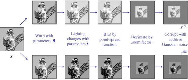
In addition to the model of Figure 1.4, however, real sensors also have associated noise in their measurements, and real images can vary in illumination as well as in their relative registrations. These factors must also be accounted for in a super-resolution model, so the full picture of how a scene or high-super-resolution image generates a low-resolution image set looks more like that of Figure 1.5.
1.2
Challenges
Super-resolution algorithms face a number of challenges in parallel with their main resolution task. In addition to being able to compute values for all the super-resolution image pixels intensities given the low-super-resolution image pixel intensities, a super-resolution system must also be able to handle:
Figure 1.5: One high-resolution image generates a set of low-resolution images. Because the images are related by sub-pixel registrations, each observation gives us more additional constraints on the values of the high-resolution image pixel intensities.
• Image registration – small image displacements are crucial for beating the sampling limit of the original camera, but the exact mappings between these images are unknown. To achieve an accurate super-resolution result, they need to be found as accurately as possible.
• Lighting variation – when the images are aligned geometrically, there may still be significant photometric variation, because of different lighting levels or camera exposure settings when the images were captured.
• Blur identification – before the light from a scene reaches the film or camera CCD array, it passes through the camera optics. The blurs introduced in this stage are modelled by a point-spread function. Separating a blur kernel from an image is an extensively-studied and challenging problem known as Blind Image Deconvolution. This can be even more challenging if the blur varies spatially across the image.
These three cases are illustrated for some low-resolution image patches in Fig-ure 1.6. While the goal is to compute a high-resolution image (e.g.as illustrated in Figure 1.1), the efficacy of any super-resolution approach depends on its handling of these additional considerations as well. Given “good” low-resolution input images, the output from an otherwise successful super-resolution algorithm will still be poor if the registration and blur estimates are inaccurate.
1.3
Thesis contributions
This thesis addresses several aspects of super-resolution by treating it as a machine learning problem.
Geometric Registration Photometric Registration Blur Estimation
Figure 1.6: Three of the challenges facing a multi-frame super-resolution algorithm. Left column: the two instances of the “P” character have different alignments, which we must know accurately for super-resolution to be possible. Middle column: the eyechart in the images has different illumination between two frames, so the photometric registration between the images also has to be estimated. Right column: the image blur varies noticeably between these two input frames, and blur estimation is a difficult challenge.
Chapter 2 gives an overview of the state of super-resolution research, and relevant literature around the field. Notation and a formal framework for reasoning about the super-resolution problem are laid out in Chapter 3, which then goes on to present new intuition about the behaviour of super-resolution approaches, giving particular consideration to uncertainty associated with registration and blur estimation, which is not something that has been addressed to this degree in other discussions of multi-frame image super-resolution.
Chapter 4 describes a simultaneous approach for super-resolution, where the geometric and photometric registration challenges are addressed at the same time as the super-resolution image estimate. This allows us to find a more accurate registration than can generally be found between two noisy low-resolution images, and the improvement in the registration estimate carries through to give a more accurate high-resolution image.
A second key point of the simultaneous super-resolution approach, also in Chap-ter 4, is the automatic tuning of parameChap-ters for an image prior at the same time as the super-resolution process. We already know that a well-chosen prior representa-tion can yield a better super-resolurepresenta-tion image, so selecting the right shape of prior becomes important, especially because most successful image priors are not easy to normalize, meaning that parameters can be difficult to learn directly.
Chapter 5 goes a step beyond what we show in the preceding chapter; rather than making a point estimate of the unknown registration parameters, we derive a method through which we can integrate them out of the problem in a Bayesian manner. This leads to a direct method of optimizing the super-resolution image pixel values, and this gives improved results which are shown both on synthetic data, where differences are easily quantified with respect to known parameters, and on real image data, which shows that the algorithm is flexible enough to be useful in real-world situations.
Chapter 6 introduces a texture-based prior for super-resolution. Using this prior,
Maximum a Posteriori super-resolution can achieve much better results on image datasets from highly textured scenes than an algorithm using a more conventional smoothness prior, and this is demonstrated on datasets with a variety of textures. This highlights the importance and power of a well-chosen representation for prior knowledge about the super-resolution image, and also shows how the patch-based methods popular in single-image super-resolution can be brought into the multi-frame setting.
The main contributions are drawn together in Chapter 7, which consolidates the main overarching themes of registration uncertainty and selection of an appropriate
research, and concludes with some final thoughts on the multi-frame image super-resolution problem.
Literature review
Image super-resolution is a well-studied problem. A comprehensive review was car-ried out by Borman and Stevenson [12, 13] in 1998, though in the intervening period a wide variety of super-resolution work has contributed to many branches of the super-resolution problem.
There are several popular approaches to super-resolution overall, and a number of different fundamental assumptions to be made, which can in turn lead to very different super-resolution algorithms. Model assumptions such as the type of motion relating the low-resolution input images, or the type of noise that might exist on their pixel values, commonly vary significantly, with many approaches being tuned to particular assumptions about the input scenes and configurations that the authors are interested in. There is also the question of whether the goal is to produce the very best high-resolution image possible, or a passable high-resolution image as quickly as possible.
either Maximum Likelihood (ML) methods, i.e. those which seek a super-resolution image that maximizes the probability of the observed low-resolution input images under a given model, orMaximum a Posteriori(MAP) methods, which make explicit use of prior information, though these are also commonly couched as regularized least-squares problems.
We begin with the historically earliest methods, which tend to represent the simplest forms of the super-resolution ideas. From these grow a wide variety of different approaches, which we then survey, turning our attention back to more detailed model considerations, in particular the ways in which registration and blur estimation are handled in the literature. Finally, we cover a few super-resolution approaches which fit less well into any of the categories or methods of solution listed so far.
2.1
Early super-resolution methods
The field of super-resolution began growing in earnest in the late eighties and early nineties. In the signal processing literature, approaches were suggested for the pro-cessing of images in the frequency domain in order to recover lost high-frequency information, generally following on from the work of Tsai and Huang [117] and later Kimet al. [67]. Roughly concurrent with this in the Computer Vision arena was the work of Peleg, Keren, Irani and colleagues [58, 59, 66, 87], which favoured the spatial domain exclusively, and proposed novel methods for super-resolution reconstruction.
2.1.1
Frequency domain methods
The basic frequency-domain super-resolution problem of Tsai and Huang [117] or Kim et al. [67] looks at the horizontal and vertical sampling periods in the digital image, and relates the continuous Fourier transform of the original scene to the dis-crete Fourier transforms of the observed low-resolution images. Both these methods rely on the motion being composed purely of horizontal and vertical displacements, but the main motivating problem of processing satellite imagery is amenable to this restriction.
The ability to cope with noise on the input images is added in by Kim et al. in [67], and Tekalp et al. [110] generalize the technique to cope with both noise and a blur on the inputs due to the imaging process.
Tom and Katsaggelos [113, 115] take a two-phase super-resolution approach, where the first step is to register, deblur and de-noise the low-resolution images, and the second step is to interpolate them together onto a high-resolution image grid. While much of the problem is specified here in the spatial domain, the solution is still posed as a Frequency domain problem. A typical result on a synthetic data sequence from [113] is shown in Figure 2.1, where the zoom factor is 2 and the four input frames are noisy.
Lastly, wavelet models have been applied to the problem, taking a similar overall approach as Fourier-domain methods. Nguyen and Milanfar [83] propose an efficient agorithm based on representing the low-resolution images using wavelet coefficients, and relating these coefficients to those of the desired super-resolution image. Boseet al.[16] also propose a method based onsecond-generationwavelets, leading to a fast algorithm. However, while this shows good results even in the presence of high levels of input noise, the outputs still display wavelet-like high frequency artifacts.
Figure 2.1: Example of Frequency-domain super-resolution taken from Tom and Katsaggelos [113]. Left: One of four synthesized low-resolution images. Right: Super-resolved image. Several artifacts are visible, particularly along image edges, but the overall image is improved.
2.1.2
The emergence of spatial domain methods
A second strand in the super-resolution story, developing in parallel to the first, was based purely in the spatial domain. Spatial domain methods enjoy better handling of noise, and a more natural treatment of the image point-spread blur in cases where it cannot be approximated by a single convolution operation on the high-resolution image (e.g. when the zoom or shear in the low-resolution image registrations varies across the inputs). They use a model of how each offset low-resolution pixel is derived from the high-resolution image in order to solve for the high-resolution pixel values directly.
The potential for using sub-pixel motion to improve image resolution is high-lighted by Peleg et al. [87]. They point out that a blurred high-resolution image can be split into 16 low-resolution images at a zoom factor of 4 by taking every 4thpixel in the horizontal and vertical directions at each of the 4×4 different offsets. If all 16 low-resolution images are available, the problem reduces to one of regular image deblurring, but if only a subset of the low-resolution frames are present, there is still
a clear potential for recovering high-frequency information, which they illustrate on a synthetic image sequence.
A method for registering a pair of images is proposed in Keren et al. [66]. The registration deals with 2D shifts and with rotations within the plane of the image, so is more general than that of [87]. However, their subsequent resampling and interpolation scheme do little to improve the high-frequency information content of the super-resolution image.
Progress was made by Irani et al.[58, 59], who used the same registration algo-rithm, but proposed a more sophisticated method for super-resolution image recov-ery based on back-projection similar to that used in Computer Aided Tomography. They also propose a method for estimating the point-spread function kernel respon-sible for the image blur, by scanning a small white dot on a black background with the same scanner.
To initialize the super-resolution algorithm, Irani et al. take an initial guess at the high resolution image, then apply the forward model of the image measurement process to work out what the observed images would be if the starting guess was correct. The difference between these simulated low-resolution images and the real input images is then projected back into the high-resolution space using a back projection kernel so that corrections can be made to the estimate, and the process repeated. It is also worth observing that at this point, the algorithms proposed for spatial-domain super-resolution all constitute Maximum Likelihood methods.
Figure 2.2: Example of early spatial-domain super-resolution taken from Irani et al. [59] (1991). Left: One of three low-resolution images (70×100 pixels) obtained using a scanner. Right: Super-resolved image. The original images were captured using a scanner.
2.1.3
Developing spatial-domain approaches
Later work by Irani et al. [60] builds on their early super-resolution work, though the focus shifts to object tracking and image registration for tracked objects, which allows the super-resolution algorithm to treat some rigid moving objects indepen-dently in the same sequence. Another similar method by Zometet al.[123] proposes the use of medians within their super-resolution algorithm to make the process ro-bust to large outliers caused by parallax or moving specularities.
The work of Rudin et al. [53, 100] is also based on the warping and resampling approach used by e.g. Kerenet al. or Ur and Gross [66, 118]. Again the transforms are limited to planar translations and rotations. The method performs well, and is simple to understand, but the way the interpolation deals with high frequencies means that the resulting images fail to recreate crisp edges well.
A good example of limiting the imaging model in order to achieve a fast super-resolution algorithm comes from Elad and Hel-Or [33]. The motion is restricted to shifts of integer numbers of high-resolution pixels (though these still represent
sub-pixel shifts in the low-resolution pixels), and each image must have the same noise model, zoom factor, and spatially invariant point-spread function, the latter of which must also be realisable by a block-circulant matrix. These conditions allow the blur to be treated afterthe interpolation onto a common high-resolution frame – this intuition is exactly the same as in [53, 100], but the work of [33] formalizes it and explores more efficient methods of solution in more depth.
2.2
Projection onto convex sets
Projection onto Convex Sets(POCS) is a set-theoretic approach to super-resolution. Most of the published work on this method is posed in an ML framework, though later extensions introduced a super-resolution image prior, making it a MAP method. However, the way in which POCS incorporates prior image constraints, and the forms such constraints take, sets this method apart from later MAP spatial-domain super-resolution methods.
POCS works by finding constraints on the super-resolution image in the form of convex sets of possible values for super-resolution pixels such that each set contains every possible super-resolution image that leads to each low-resolution pixel under the imaging model. Any element in the intersection of all the sets will be entirely consistent with the observed data.
An early ML form of POCS was proposed by Stark and Oskoui in 1989 [105], thus it emerged only just later than the “early” methods covered in Section 2.1. In the same paper that commented on early frequency-domain super-resolution, Tekalp et al. [110] also proposed extensions to POCS super-resolution to include a noise model. Later work by Pattiet al.[85, 86] extended the family of homographies
considered for the image registration, and also allowed for a spatially-varying point-spread function. The linear model relating low- and high-resolution pixels is closely related to that used in later fully-probabilistic super-resolution approaches, and in general POCS it is a strong and successful method.
Like the other super-resolution approaches, the POCS method has been applied and extended in number of different directions: Eren [34] et al. extend [85, 86] for cases of multiple rigid objects moving in the scene by using validity or segmen-tation maps, though it uses pre-registered inputs; Elad and Feuer [29] propose a hybridized ML/MAP/POCS scheme which optimizes a differently-formulated set of convex constraints including the usual ML least-squares formulation along with other POCS-style solution constraints; Patti et al., and also Elad and Feuer [30, 31, 32] use Kalman filtering to pose the problem in a way which is computationally efficient to solve; and Patti and Altunbasak [84] consider a scheme to include a constraint in the POCS method to represent prior belief about the structure of the recovered high-resolution image, making it a MAP estimator.
Figure 2.3: An example of POCS super-resolution taken from Pattiet al. [86]. Left: four of twelve low-resolution images, which come from six frames of interlaced low-resolution video captured with a hand-held camcorder. Middle: interpolated approximation to the high-resolution image. Right: super-resolution image found using Patti et al.’s POCS-based super-resolution algorithm.
2.3
Methods of solution
One factor motivating the choice of any particular super-resolution method for an application is the cost of the computation associated with the various different meth-ods, and how likely they are to converge to a unique optimal solution.
The early Frequency-domain methods, such as that of Kimet al.[67], are posed as simple least-squares problems (i.e. of the type Ax = b), hence are examples of
convex functions for which a unique global minimum exists. The super-resolution estimate is found using an iterative re-estimation process, e.g. gradient descent. In contrast, the projection-based work of Irani et al. [58, 59] was reported to yield several solutions depending on the initial image guess, or to oscillate between several solutions rather than converging onto one.
The capabilities of the standard ML estimator are explored by Capel in [21] (see also Section 3 of this thesis), and this is another classic linear system. We can find this spatial ML super-resolution estimate directly by using the pseudoinverse, though this is a computationally expensive operation for large systems of image pixels, so cheaper iterative methods are generally preferred. Since this is another convex problem, the algorithm is guaranteed to converge onto the same global optimum whatever the starting estimate, though a poor initial super-resolution image may mean that many more iterations are needed.
In POCS super-resolution, as in Tekalp et al. [110], the high-resolution image is found using another iterative projection technique. The constraints from the low-resolution images form ellipsoids in the space spanned by all the possible high-resolution pixel values. Other constraints, like bounds on acceptable pixel intensity values, can also be added, but will not necessarily be ellipsoids. As long as the
constraints are convex and closed, then projecting onto each of the sets of constraints in turn, cyclically, guarantees convergence to a solution satisfying all the constraints.
2.4
Maximum a posteriori
approaches
Most super-resolution problems now are either explicitMaximum a Posteriori(MAP) approaches, or are approaches that can be re-interpreted as MAP approaches be-cause they use a regularized cost function whose terms can be matched to those of a posterior distribution over a high-resolution image, as the regularizer can be viewed as a type of image prior.
If a prior over the high-resolution image is chosen so that the log prior distribution is convex in the image pixels, and the basic ML solution itself is also convex, then the MAP solution will have a unique optimal super-resolution image. This makes the convexity-preserving priors an attractive choice, though we will touch on various other image priors as well.
In the error-with-regularizer framework, a popular form of convex regularizer is a quadratic function of the image pixels, like kAxk22, for some matrixA and image pixel vector x. If the objective function is exponentiated, it can be manipulated to give the probabilistic interpretation, because a term like exp−1
2 kAxk 2
2 is pro-portional to a zero-mean Gaussian prior over x with covariance ATA. These are examples of Gaussian Markov Random Field (GMRF) priors, because they assume that the distribution of high-resolution pixels can be captured as a multivariate Gaussian. Many types of GMRFs can be formulated, depending on the correlation structure they assume over the high-resolution image.
Figure 2.4: Cheeseman et al.’s MAP approach, applied to data from the Viking Orbiter. Figure taken from [23]. Left: one of 24 input frames. Centre: their “composite image” (same as theaverage imagelater used by Capel [21]). Right: MAP super-resolution result.
see that these are not always the best choices for image super-resolution, and a number of superior options can be found without having to sacrifice the benefits of having a prior convex in the image pixel values.
2.4.1
The rise of MAP super-resolution
In a powerful early example of MAP super-resolution Cheeseman et al. [23] pro-posed a Bayesian scheme to combine sets of similar satellite images of Mars using a Gaussian prior in a MAP setting. The prior simply assumed each pixel in the high-resolution image was correlated with its four immediate neighbours on the high-resolution grid. Cheeseman et al. illustrated that while their prior is a poor model for earth satellite imagery, the Martian images did give rise to intensity dif-ference histograms that are approximately Gaussian. Figure 2.4 shows their result
on Viking Orbiter data.
In another relatively early MAP super-resolution paper, Hardie et al. use the L2 norm of a Laplacian-style filter over the super-resolution image to regularize their MAP reconstruction. Again, this forms a Gaussian-style prior (viewing the Laplacian-style filter as matrix A in the example above). In addition to finding a MAP estimate for the super-resolution image, Hardie et al. also found a maximum likelihood estimate for the shift-only image registration at the same time [56].
2.4.2
Non-Gaussian image priors
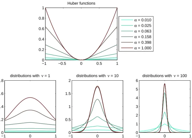
Schultz and Stevenson [101, 102] look at video sequences with frames related by a dense correspondence found using a hierarchical block-matching algorithm. Rather than a simple Gaussian prior to regularize the super-resolution image recovery, they use a Huber Markov Random Field (HMRF). The first or second spatial derivative of the super-resolution image is found, and the Huber potential function is used to penalize discontinuities. The Huber function is quadratic for small values of input, but linear for larger values (see Section 3.4.2 and Figure 3.12), so it penalizes edges less severely than a Gaussian prior, whose potential function is purely quadratic. This Huber function models the statistics of real images more closely than a purely quadratic function, because real images contain edges, and so have much heavier-tailed first-derivative distributions than can be modelled by a Gaussian.
Farsiuet al.[35, 36, 37, 38] move to the other extreme, and base their image prior on the L1 norm, referred to asTotal Variation(TV) priors. This leads to a function that can be computed very rapidly because there is no multiplication involved, unlike the Gaussian and Huber-MRF priors, which involve squared terms. The authors’
Figure 2.5: Farsiu et al.’s fast and robust SR method, using a TV prior, taken from [37]. Left and Centre: input images 1 and 50 from a 55-image sequence. Right: output of their robust method with a TV prior. Notice that while the method is highly over-constrained, their approach is constructed in such a way as to create a consistent super-resolution image even thought the camel in the image moves independently of the rest of the scene in a few of the frames.
main stated aim is speed and computational efficiency, and they explore several ways of formulating quick solutions by working withL1 norms, rather than the more common L2 norms, to solve the super-resolution problem. One set of their results with their “fast and robust” super-resolution method is given in Figure 2.5. Ng et al.also use the TV prior [78] for super-resolving digital video sequences, though they also assume Gaussian noise (i.e. L2 errors on the term involving the low-resolution images). They compare their TV regularization to Laplacian regularization (a form of GMRF), and show that the TV regularization gives more favourable signal-to-noise ratios on the reconstructed super-resolution images.
Capel and Zisserman [20] compare the back-projection method of Irani and Peleg to simple spatial-domain ML approaches, and show that these perform much less well on a text image sequence than the HMRF method, and also to a regularized
Total Variation (TV) estimator. Later they also show that the simple constraint of bounding the image pixel values in the ML solution improves the solution signifi-cantly [18] (see also Section 3.3.1 and Figure 3.6 of this thesis).
Other work by Capel and Zisserman [17, 18] considers super-resolution as a second step after image mosaicing, where the image registration (using a full
8-Figure 2.6: Capel’s face super-resolution, taken from [21]. Left: one of thirty synthetic low-resolution input images at a zoom factor of three. Centre-left: the Huber-MRF reconstruction. Centre-right: MAP reconstruction using PCA faces and a face-space prior. Right: MAP reconstruction using PCA faces and an image-space prior.
degrees-of-freedom projective homography) is carried out in the mosaicing step. Also proposed [18, 21] are high-resolution image priors for dealing specifically with faces by building up aPrincipal Component Analysis(PCA) representation from training data. The face is divided into 6 regions, and eigenimage elements learnt for each. This information is then included as priors either by constraining the high resolution image to lie near the PCA subspace, using an optimization algorithm to optimize over all possible super-resolution images, or by constraining the solution to lie within the subspace but making use of the variance estimates for each principal component. In the latter case, the optimization need only be over the component weightings, so the dimension of the problem is considerably smaller than if each high-resolution pixel were considered individually. Some of Capel’s results are shown in Figure 2.6. This method is extended by Gunturk et al.[55] to carry out face recognition using a face feature vector obtained directly from the low-resolution images using a similar super-resolution process.
As well as faces, a number of authors have concentrated on improving functions to encode prior knowledge for particular super-resolution applications, such as text-reading. A bimodal prior was suggested by Donaldson and Myers [27], because text
images tend to contain mainly black or white pixels. Fletcher et al. create a super-resolution system particularly for reading road signs [42], and also use text-specific prior knowledge in their algorithm.
The work of Baker and Kanade [4, 5, 6] offers a careful analysis of the sources of noise and poor reconstruction in the ML case, by considering various forms of the point spread function and their limitations. The MAP formulation of super-resolution is introduced with the suggestion of recognition-based super-super-resolution. This method works by partitioning the low-resolution space into a set of classes, each of which has a separate prior model. For instance, if a face is detected in the low resolution image set, a face-specific prior over the super-resolution image will be used. The low-resolution classification is made by using a pyramid of multi-scale Gaussian and Laplacian images built up from training data, and the specific priors are imposed by constraining the gradient in the super-resolution image to be as close as possible to that of the closest-matching pyramid feature vector. Example results show that even with inputs of constant intensity, given a face-specific prior, their algorithm will “hallucinate” a face into the super-resolution image.
Various attempts have been made to put bounds on the utility of super-resolution techniques; Baker and Kanade discussed the limits in [4, 6], and more recently Lin and Shum formalized limits for super-resolution under local translation [70], though in this case only for a “box” point-spread function. Most cases for which theoretical limits can be derived are considerably less complex than super-resolution algorithms used in practice.
2.4.3
Full posterior distributions
A more recent trend in MAP super-resolution has been to take the full posterior distribution of the super-resolution image into account, rather than just taking the maximal posterior value as the single image estimate. This is only possible for a subset of the useful priors on the image, and generally Gaussian priors are used in spite of the fact they tend to produce over-smooth results. Finding the covariance of the high-resolution intensity values is useful in making further estimates, especially in estimating imaging parameters.
Woodset al.[121] present an iterative EM (Expectation Maximization) algorithm for the joint registration, blind deconvolution, and interpolation steps which also es-timates the blur, noise, and motion parameters. All the distributions in the problem setup are assumed Gaussian, so the posterior is also Gaussian. The covariance ma-trix is very large, and the EM update equations require the evaluation of the inverse of this matrix. By using Fourier domain methods (as described in 2.1.1) along with some fairly severe restrictions on their forward model (integer high-resolution-pixel shifts only, with all images sharing the same zoom, blur and decimation), they are able to derive direct updates for both the image noise parameter and the parameter governing the Gaussian prior on the super-resolution image.
Finally, Tipping and Bishop [112] take a different view of super-resolution and marginalize out the unknown super-resolution image to carry out the image registra-tion using exactly the same model structure as the MAP super-resoluregistra-tion problem. Again, a Gaussian form of the prior over the super-resolution image is selected in order to make this possible; a more sophisticated prior like the Huber-MRF would lead to an intractable integral. Unlike [121], Tipping and Bishop do evaluate the spatial-domain matrices, though because of the computational restrictions, they use
very small low-resolution images of 9×9 low-resolution pixels in the part of their algorithm where they perform parameter estimation.
2.5
Image registration in super-resolution
Almost all multi-frame image super-resolution algorithms need to have some es-timate of the motion relating the low-resolution input frames. There are a very small number of reconstruction-based super-resolution approaches which do not use motion, but instead employ changes in zoom (Joshi et al. [64, 65]) or defocus (Ra-jagopalan and Chaudhuri [95, 96]) in order to build up the constraints on the high-resolution image pixel intensities necessary to estimate the super-high-resolution image.
Within the vast majority of methods which do use sub-pixel image motion as the main cue for super-resolution, many authors assume that the image registration problem is solved to a sufficient degree that a satisfactory image registration is available a priori, so the registration process requires little to no direct discussion. Other authors describe the registration schemes they use, and of particular interest are the methods which take account of the super-resolution model in order to improve the registration estimates.
A typical method for registering images is to look for interest points in the low-resolution image set, then use robust methods to estimate the point correspon-dences [41, 116] and compute homographies between images. In an early super-resolution paper, Irani and Peleg [58] used an iterative technique to warp the low-resolution images into each others frames to estimate registration parameters (in this case two shifts and a rotation per image) prior to the super-resolution reconstruction phase. Other authors use hierarchical block-matching algorithms to register their
Figure 2.7: Hardie et al.’s joint registration and super-resolution, taken from [56]. Left: one of the sixteen infra-red low-resolution image inputs. Right: the high-resolution MAP image estimate.
input images, again as an independent step prior to the actual super-resolution reconstruction [102].
Hardie et al. [56] made use of the super-resolution image estimate in order to refine the registration of the low-resolution images. They restricted the motion model to be shifts of integer numbers of high-resolution image pixels, and searched over the grid of possible alignments for each low-resolution image between iterations of their MAP reconstruction algorithm. Example images taken from [56] are shown in Figure 2.7.
Much more recently, Chung et al. [25] revisited this idea, using an affine regis-tration. The imaging model they select falls into the trap of resampling the high-resolution image using bilinear interpolation in the high-high-resolution frame before applying a second operation to average over high-resolution pixel values in order to produce their low-resolution frames. As Capel [18] explains, this can give a poor ap-proximation to the generative model. This is likely to occur when the image registra-tion causes a change in zoom factor, or perspective foreshortening (though Chunget al.’s model is only affine). However, even with the limitations of their model, the
au-thors show that considering the registration and super-resolution problems together, a more accurate super-resolution image estimate can be obtained.
Tipping and Bishop [112] searched a continuous space of shift and rotation pa-rameters to find the parameter settings which maximized the marginal data like-lihood, which takes into account the super-resolution image’s interaction with the low-resolution images, even though the exact values of the super-resolution image intensities have themselves been integrated out of the problem in their formulation. Once Tipping and Bishop have estimated the registration, a more conventional MAP reconstruction algorithm is used to estimate the high-resolution image.
All these cases use parametric estimates for the image registration, generally with low numbers of registration parameters per image. At the other end of the spectrum, a number of super-resolution algorithms use optic flow to estimate the motion of each pixel using dense image-to-image correspondences [3, 44, 50, 78, 122]. It is not just the geometric registration which can change between the low-resolution images. Changes in scene illumination or in camera white balance can lead to photometric changes as well. Capel [18] makes a linear photometric registra-tion estimate per image, based on fitting a linear funcregistra-tion to pixel correspondences obtained after a geometric registration and warping into the same frame. More re-cently, Gevrekci and Gunturk [51] have also used a linear photometric model fitted after geometric registration in order to improve the dynamic range of input images acquired over highly variable lighting conditions.
2.6
Determination of the point-spread function
Diffraction-limited optical systems coupled with sensors of various geometries lead to a variety of possible point-spread function shapes [11, 15, 50]. Unfortunately, except for rare super-resolution applications where the imaging hardware can be entirely calibrated ahead of time and is then used to image a static scene, most super-resolution applications face some uncertainty about the exact shape of the point-spread function. In a few cases, the blur can be estimated by measuring the blur on step edges or point light sources in the image, or by taking additional calibration shots [76], but for most applications, determination of the point-spread function is a hard problem.
Blind image deconvolution is a closely-related problem, in which the goal is to take an image blurred according to some unknown kernel, and separate out the underlying source image and the kernel image, using no further inputs. A review of Blind Image Deconvolution is given in [68], though many of the methods are not entirely suitable for real super-resolution applications; for example, zero sheet separation is highly sensitive to noise and prone to numerical inaccuracy for large datasets, and the performance of frequency domain methods also suffers when im-age noise masks the nulls in the imim-age Fourier transform which would otherwise contain information about the blur function. The two most appropriate methods for super-resolution PSF determination are those with the best ability to cope with image noise, and these are Reeves and Mercereau’s “Blur identification by general-ized cross-validation” [99], and Lagendijk et al.’s “Maximum Likelihood image and blur identification” [69].
Cross-validation approaches are widely used to tune model parameters by examining how well a model learned on one subset of the data performs on another disjoint subset, and Generalized Cross-Validation (GCV) extends the leave-one-out variant of this (where the data used in evaluation consist of each element alone in turn). The GCV blur identification method was taken up in multi-frame image super-resolution by Nguyen et al. [79, 80, 81, 82, 83], who consider the blur identification and im-age restoration problem as a special case of imim-age super-resolution where the low-resolution pixels all lie on a fixed grid. They also extend the blur-learning method to handle the learning of a prior strength parameter for image super-resolution.
The maximum likelihood approach for blur identification is used both in Tipping and Bishop’s “Bayesian image super-resolution” [112], and in Abadet al.’s “ Param-eter estimation in super-resolution image reconstruction” [1] (and similarly [75]). Both pieces of work begin with a Gaussian data error function and a Gaussian im-age prior over the super-resolution imim-age, then integrate the super-resolution imim-age out of the problem to leave an equation that can by maximized with respect to the variables of interest. In the case of [112], this is the PSF standard deviation and some geometric image registrations; for [1] this is a selection of PSF values and a parameter governing the strength of the prior on the high-resolution image.
Wanget al.[120] use a MAP expression for the PSF parameter, a strong patch-based high-resolution image prior, and importance re-sampling to obtain values for the PSF parameter from its approximate distribution.
Recently, Variational Bayes has been applied both in the field of blind image deconvolution and in super-resolution. Original work by Miskin and MacKay [73] deals with blind source separation and blur kernel estimate. This is extended by Fergus et al. [39] to cover a much wider class of photographic images. The
de-Figure 2.8: Molina et al.’s blind deconvolution using a variational approach to recover the blur and the image. Left: astronomical image displaying signifi-cant blur. Centre and Right: Two possible reconstructions; images taken from [74]. convolution approach of Molina et al. [74] is also similar to Miskin and MacKay’s deblurring work, and builds on the Variational Bayes approach to blur determina-tion in super-resoludetermina-tion. Figure 2.8 shows a blurred astronomical image, and two possible restored images from [74].
2.6.1
Extensions of the simple blur model
Most of the PSF determination techniques mentioned above relate to the estimation of parameters for blurs from specific families like Gaussians or circular blur functions, and only the variational work [39, 73, 74] builds up a non-parametric pixel-wise representation of the blur.
In between the simple one-parameter blur model and the full pixel-wise represen-tation, several bodies of work model motion blur in addition to Gaussian or circular PSFs, making use of the motion of an input video sequence [7, 24, 50, 98].
The image blur plays a key role in depth-from-defocus, where several differently-defocused images are used to estimate a depth map. The extent of the spatially varying PSF for any point in the image is related to the depth of the object in the scene, and some camera parameters. Given that the depth stays the same while the camera parameters are varied, one can acquire several samples with different parameters and then eliminate the unknowns. The problem can be solved in several
ways, both in the image domain with MRFs and in the spatial frequency domain [95, 96]. The main drawback of this approach is that the available data must include several differently-focused frames, and suitably large changes of focus may not occur in a general low-resolution image sequence.
2.7
Single-image methods
Single-image super-resolution methods cannot hope to improve the resolution by overcoming the Nyquist limit, so any extra detail included in the high-resolution image by such algorithms must come from elsewhere, and prior information about the usual structure of a high-resolution image is consequently an important source. The single-image super-resolution method proposed by Freemanet al.[45] is con-sidered state-of-the-art. It learns the relationship between low- and high-resolution image patches from training data, and uses a Markov Random Field (MRF) to model these patches in an image, and to propagate information between patches using Belief Propagation, so as to minimize discontinuities at high-resolution patch boundaries. This work is based on the framework for low-level vision developed by Freeman et al. [46, 47, 48, 49].
Tappenet al.[109] also use Belief Propagation to produce impressive single-image super-resolution results, this time exploiting a high-resolution image prior based on natural image statistics to improve the image edge quality in the high-resolution outputs. The example in Figure 2.9 shows results from [109] for both this method and the original Freeman et al. [45] example-based super-resolution method.
An undisclosed algorithm in a commercial Photoshop plug-in, Genuine Fractals, by LizardTech [43], is also used as a benchmark for single-image super-resolution
Figure 2.9: Tappen et al.’s sparse derivative prior super-resolution (taken from [109]). Left: Original image, before being decimated to have half the number of pixels in each dimension. Centre: The result of performing Freeman et al.’s single-image super-resolution method on the low-resolution single-image. Right: the result of using Tappen et al.’s sparse derivative prior super-resolution.
(see Figure 1.3). The method is not based on training data from other images, and it is marketed as being able to resize images to six hundred percent of the original without loss of image quality, though [45] states that it suffers from blur in textured regions and fine lines.
A method by Storkey [106] was inspired by work on structural image analy-sis [107]. Rather than using a model for the blur or image degradation during the imaging procedure, a latent image space is formed, and links are dynamically cre-ated between nodes in this space and the low- and high-resolution images. The method is restricted to a fixed zoom factor, and the resulting image has very sharp edges where there is a boundary between regions of the high-resolution image that are influenced by different latent nodes.
Sunet al. [108] perform what they termImage Hallucination on individual low-resolution images to obtain low-resolution output images in which plausible high-resolution details have been invented based on a “primal sketch” prior constructed from several unrelated high-resolution training images. The results display plausible levels of high-frequency information in the image edges at a zoom factor of three
in each spatial direction, though in some cases appear to suffer from an edge over-sharpening phenomenon similar to that described above.
Jiji et al. [62, 63] work with wavelet coefficients as an image representation, rather than using the pixel values in various frequency bands to estimage high-frequency image components as in Freeman et al.’s work. Wavelets allow for more localized frequency analysis than global image filtering or fourier transforms, though regularization is required to keep the outputs visually smooth and free from wavelet artifacts. Such single-frame wavelet methods are also improved upon by Temizal and Vlachos [111], who use local corellations in wavelet coefficients to improve their performance.
Finally, Begin and Ferrie [8] suggest an extension to the Freeman et al. [45] which deals with the estimation of the PSF and tries to take uncertainty in the parameter value into account. The blur estimate itself is made using the Lucy-Richardson algorithm, but the dictionary of patches used in the super-resolution phase is constructed from image pairs where the low-resolution image has been subjected to a range of blurs concentrated around the kernel size found using Lucy-Richardson.
It is important to note that while none of these single-image methods needs to perform registration/motion estimation between multiple inputs, these methods still highlight the great importance of having a good model and of exploiting prior knowledge about working in the image domain.
2.8
Super-resolution of video sequences
A common source of input data for super-resolution algorithms is digital video data, where the goal is either to capture one high-resolution still frame from a low-quality video sequence, or to produce an entire high-definition version of the video itself.
Several authors who tackle this problem simply employ POCS-based super-resolution image reconstruction, or techniques based on iterated back-projection [61], but there are additional constraints which can generally be exploited in video super-resolution. In [14], Borman and Stevenson use a Huber-MRF prior not only in the spatial domain, as described in 2.4.2, but also in the temporal domain at the same time by using a finite difference approximation to the second temporal derivative.
The ability to deal with the full spatio-temporal structure is also exploited by Schechtman et al. [103, 104] in considering Space-Time Resolution; they consider a space-time volume swept out by a video sequence and seek to increase the resolution along the temporal axis as well as the spatial axes by taking multiple videos as sources. An example of the temporal aspect of their super-resolution is shown in Figure 2.10.
Figure 2.10: Examples of Schechtman et al.’s space-time super-resolution, which appears in [103] and [104]. Left and centre: two of 18 input images with low frame-rates. Right: an output image which has been super-resolved in time, so that the path of the bouncing basket ball can be seen even more clearly.
Another space-time application is described by Pelletier et al. [88], who use a super-resolution model to combine two video streams. High-resolution frames are available at a very low frame rate, low-resolution frames are available at a higher frame rate, and the goal is to synthesize a high-resolution, high-frame-rate output video.
An interesting challenge in video super-resolution is introduced when video input sequences are compressed, e.g. by being saved in the MPEG video format. Some methods designed especially to work with digital video take advantage of this by modelling the discrete cosine transform component of the video compression algo-rithms directly, and by taking into account the quantization that the compression involves [2, 54].
Finally, Bishopet al.[10] propose a video super-resolution method for improving on the spatial resolution of a video sequence using a hallucination method which is most closely related to the single-image methods of the previous section. High-resolution information for each patch in the low-High-resolution frames is suggested by matching medium-resolution candidates from a dictionary, and consistency is en-forced both spatially, to make each frame a plausible image, and temporally, to minimize flicker in the resulting video sequence.
2.9
Colour in super-resolution
Early approaches to colour in super-resolution tended to concentrate on how to extend the grey-scale algorithm to handle colour images where each pixel had a three-value colour. Irani et al. [59] transformed the colours into a YIQ (luminance and chrominance) representation, and carried out most of the work only on the
Figure 2.11: The Bayer pattern on a sensor (image obtained from Wikipedia under the GNU Free Documentation License).
luminance component. Later, Tom and Katsaggelos [114] used the additional colour channels to improve their image pre-registration step, noting that registering each colour channel separately can give rise to three different registrations between a single pair of images.
More recently, attention has been paid to the way in which pictures are created. When a digital camera images a scene, it typically senses red, green and blue chan-nels spatially separately, giving rise to a colour-interleaved Bayer pattern, as shown in Figure 2.11. Most cameras compensate for this as an internal processing step, but algorithms have been developed to treat this demosaicingproblem in a similar way to the inference of high-resolution pixel values in super-resolution; the offset grids of red, green and blue measurements bear certain similarities to offset low-resolution images, and in the case of Bayer patterns in cameras, the offsets involved are known to a high degree of accuracy because of the geometry of the CCD array.
In [109], Tappenet al. use the same natural image prior and belief propagation approach they use for super-resolution on the colour demosaicing problem and show convincing results. Vegaet al.[119] also follow a probabilistic super-resolution model to improve interpolation from a single Bayer-pattern low-resolution image. For the multi-frame super-resolution setting, a colour model accounting for the Bayer
pat-tern is used by Farsiu et al. [37, 35], and again significant improvements are shown when the model takes the colour pattern into account. Note however that the model is only applicable when digital inputs are captured using a Bayer-pattern camera, and subsequently saved in an uncompressed format; general low-resolution colour datasets will not necessarily meet these criteria, e.g. if the low-resolution images have been saved as lossy JPEG images, or captured using traditional film cam-eras (e.g. scanned movie film), or with other digital imaging devices which employ different colour filtering.
2.10
Image sampling and texture synthesis
Methods such as Freeman et al.’s example-based super-resolution [45], discussed above, work well because the high-resolution information missing from the low-resolution inputs is recovered using data sampled from other images. This patch-sampling method had not previously been used in multiple-image super-resolution because most schemes rely on parametric priors which lead to simple and quick optimization schemes.
One of the contributions of the work presented in this thesis, published initially in [92], is to apply sample-based priors to multiple-image super-resolution. The prior we use is based on the texture synthesis scheme of Efros and Leung [28]. While classical texture synthesis methods work by characterizing statistics, filter responses, or wavelet descriptions of sample textures, then using these to generate new texture samples, the approach of [28] recognizes that the initial texture sample itself can be used to represent a probability model for the texture distribution directly by sampling.
First, the square neighbourhood around the pixel to be synthesized (excluding any regions where there texture has not yet been generated) is compared with similar regions in the sample image, and the closest few (all those within a certain distance) are used to build a histogram of central pixel values, from which a value for the newly-synthesized pixel is drawn. The synthesis proceeds one pixel at a time until all the required pixels in the new image have been assigned a value.
This algorithm has one main variable factor which governs its overall behaviour, and that is its definition of the neighbourhood, which is determined both by the size of the square window used, and by a Gaussian weighting factor applied to that window, so that pixels near to the one being synthesized carry more weight in the matching than those further away.
Even more recent work on patch-based super-resolution has been carried out by Wang et al. [120], who use strong sample-based priors to estimate even the image point-spread function in a MAP setting. Multi-image versions of a system similar to that used by Freeman et al. in [45] are applied by Rajaram, Das Gupta and colleagues [26, 97], though in these cases the authors constrain the problem by using low-resolution images with a precise regular spacing on a grid, reducing the motion model to be the same constrained translation-only motion model often used in frequency-domain super-resolution approaches.
The anatomy of super-resolution
This chapter introduces the notation used for the remainder of the thesis. We use a generative model to describe the image formation process in terms of a motion model and camera optics, and we cover some of the standard image priors used in super-resolution. The second purpose of this chapter is to bring out more of the structure of the general multiframe super-resolution problem, in order to motivate the approaches followed subsequently.
The data available to us are low-resolution images of a single scene. In order to work with these, we need to know about their alignment to one another, the extent of any lighting variations between images in the set, and the kind of blur, discretization and sampling that have been introduced during the imaging process. Thus we have a single scene (high-resolution image), linked to several low-resolution images through several geometric and photometric transforms.
3.1
The generative model
A generative model is a parameterized, probabilistic model of data generation, which attempts to capture the forward process by which observed data (in this case low resolution images) is generated by an underlying system (the scene and imaging parameters), and corrupted by various noise processes. This translates to a top-down view of the super-resolution problem, starting with the scene or high-resolution image, and resulting in the low-resolution images, via the physical imaging and noise processes.
For super-resolution, the generative model approach is intuitive, since the goal is to recover the initial scene, and an understanding of the way it has influenced the observed low-resolution images is crucial. The generative model’s advantage over classical descriptive models is that it allows us to express a probability distribution directly over the “hidden” high-resolution image given the low-resolution inputs, while handling the uncertainty introduced by the noise.
A high-resolution scene x, with N pixels (represented as an N ×1 vector), is assumed to have generated a set of K low-resolution images, where the kth such image is y(k), and has M pixels. The warping, blurring and subsampling of the scene is modelled by an M ×N sparse matrix W(k) [18, 112], and a global affine photometric correction results from multiplication and addition across all pixels by scalars λ(1k) and λ(2k) respectively [18]. Thus the generative model for one of the low-resolution images is
where1is a vector of ones, and the final term on the right is a noise term consisting of i.i.d. samples from a zero-mean Gaussian with precision β, or alternatively with standard deviation σN, where β−1 = σ2N. This generative model is illustrated in
Figure 3.1 for two images with differences in the geometric and photometric param-eter values, leading to two noticeably different low-resolution images from the same scene.
Figure 3.1: The generative model for two typical low-resolution images.
On the left is the single ground truth scene, and on the extreme right are the two images (in this case y(1) and y(K), which might represent the first and last images in a K-image sequence) as they are observed by the camera sensors.
The generative model for a set of low-resolution images was shown in Figure 1.5. Given a set of low resolution images like this,y(k) , the goal is to recoverx, without knowing the values associated with W(k),λ(k), σN .
3.2
Considerations in the forward model
While specific elements ofWare unknown, it is still highly structured, and generally can be parameterized by relatively few values compared to its overall number of
non-zero elements, though this depends upon the type of motion assumed to exist between the input images, and on the form of the point-spread function.
3.2.1
Motion models
Early super-resolution research was predominantly concerned with simple motion models where the registration typically had only two or three degrees of freedom per image, e.g.from datasets acquired using a flatbed scanner and an image target. Some models are even more restrictive, and in addition to the 2DoF shift-only registration, the low-resolution image pixel centres are assumed to lie on a fixed integer grid on the super-resolution image plane [56, 83].
Affine (6DoF) and planar projective (8DoF) motion models are generally appli-cable to a much wider range of common scenes. The 8DoF case is most suitable for modelling planar or approximately planar objects captured from a variety of angles, or for cases where the camera centre rotates about its optical centre, e.g. during a panning shot in a movie.
However, some real-world examples, like 3D scenes with translating cameras, will still be a problem for registrations based on homographies, because of multiple motions and occlusion. In these cases, optic flow methods are used to estimate flow of image intensity from one shot to the next in the form of a vector field. Such models use visibility masks to handle occlusions, which are then dealt with as a special case in the super-resolution algorithm.
Most of the work in this thesis is based upon planar projective homographies, since the model applies to a wide variety of interesting problems. Additionally, small image regions and short time sequences can often be adequately approximated using
![Figure 2.4: Cheeseman et al.’s MAP approach, applied to data from the Viking Orbiter. Figure taken from [23]](https://thumb-us.123doks.com/thumbv2/123dok_us/9228094.2407739/28.892.150.767.204.515/figure-cheeseman-approach-applied-viking-orbiter-figure-taken.webp)