The Configurable SAT Solver Challenge (CSSC)
Frank Huttera, Marius Lindauera, Adrian Balintb, Sam Baylessc, Holger Hoosc, Kevin Leyton-Brownc
aUniversity of Freiburg, Germany bUniversity of Ulm, Germany
cUniversity of British Columbia, Vancouver, Canada
Abstract
It is well known that different solution strategies work well for different types of instances of hard combinatorial problems. As a consequence, most solvers for the propositional satisfiability problem (SAT) expose parameters that allow them to be customized to a particular family of instances. In the international SAT competition series, these parameters are ignored: solvers are run using a single default parameter setting (supplied by the authors) for all benchmark instances in a given track. While this competition format rewards solvers with robust default settings, it does not reflect the situation faced by a practitioner who only cares about performance on one particular application and can invest some time into tuning solver parameters for this application. The new Configurable SAT Solver Competition (CSSC) compares solvers in this latter setting, scoring each solver by the performance it achieved after a fully automated configuration step. This article describes the CSSC in more detail, and reports the results obtained in its two instantiations so far, CSSC 2013 and 2014.
Keywords: Propositional satisfiability, algorithm configuration, empirical evaluation, competition
1. Introduction
The propositional satisfiability problem (SAT) is one of the most prominent problems in AI. It is relevant both for theory (having been the first problem proven to be NP-hard [27]) and for practice (having important applications in many fields, such as hardware and software verification [19, 72, 26], test-case generation [79, 24], AI planning [53, 54], scheduling [28], and graph colouring [84]). The SAT community has a long history of regularly assessing the state of the art via competitions [50]. The first SAT competition dates back to the year
Email addresses: [email protected](Frank Hutter),
[email protected](Marius Lindauer),[email protected](Adrian Balint),[email protected](Sam Bayless),[email protected](Holger Hoos),
2002 [76], and the event has been growing over time: in 2014, it had a record participation of 58 solvers by 79 authors in 11 tracks [13].
In practical applications of SAT, solvers can typically be adjusted to perform well for the specific type of instances at hand, such as software verification instances generated by a particular static checker on a particular software system [3], or a particular family of bounded model checking instances [86]. To support this type of customization, most SAT solvers already expose a range of command line parameters whose settings substantially affect most parts of the solver. Solvers typically come with robust default parameter settings meant to provide good all-round performance, but it is widely known that adjusting parameter settings to particular target instance classes can yield orders-of-magnitude speedups [42, 55, 81]. Current SAT competitions do not take this possibility of customizing solvers into account, and rather evaluate solver performance with default parameters.
Unlike the SAT competition, theConfigurable SAT Solver Challenge (CSSC) evaluates SAT solver performanceafterapplication-specific customization, thereby taking into account the fact that effective algorithm configuration procedures can automatically customize solvers for a given distribution of benchmark in-stances. Specifically, for each type of instancesT and each SAT solverS, an automated fixed-time offline configuration phase determines parameter settings ofS optimized for high performance onT. Then, the performance of S onT is evaluated with these settings, and the solver with the best performance wins.
To avoid a potential misunderstanding, we note that for winning the compe-tition, only solver performance after configuration counts, and that it doesnot matter how much performance was improved by configuration. As a consequence, in principle, even a parameterless solver could win the CSSC if it was very strong: it would not benefit from configuration, but if it nevertheless outperformed all solvers that were specially configured for the instance families in a given track, it would still win that track. (In practice, we have not observed this, since the improvements resulting from configuration tend to be large.)
The competition conceptually most closely related to the CSSC is the learning track of the international planning competition (IPC, see, e.g., the description by Fern et al. [31]1, which also features an offline time-limited learning phase on training instances from a given planning domain and an online testing phase on a disjoint set of instances from the same domain. The main difference between this IPC learning track and the CSSC (other than their focus on different problems) is that in the IPC learning track every planner uses its own learning method, and the learning methods thus vary between entries. In contrast, in the CSSC, the corresponding customization process is part of the competition setup and uses the same algorithm configuration procedure for each submitted solver. Our approach to evaluating solver performance after configuration could of course be transferred to any other competition. (In fact, the 2014 IPC learning track for non-portfolio solvers was won by FastDownward-SMAC [75], a system that
1
http://www.cs.colostate.edu/~ipc2014/
employs a similar combination of general algorithm configuration and a highly parameterized solver framework as we do in the CSSC.)
In the following, we first describe the criteria we used for the design of the CSSC (Section 2). Next, we provide some background on the automated algorithm configuration methods we used when running the competition (Section 3). Then, we discuss the two CSSCs we have held so far (in 2013 and 2014); we discuss each of these competitions in turn (Sections 4 and 5), including the specific benchmarks used, the participating solvers, and the results. We describe two main insights that we obtained from these results:
1. In many cases, automated algorithm configuration found parameter settings that performed much better than the solver defaults, in several cases yielding average speedups of several orders of magnitude.
2. Some solvers benefited more from automated configuration than others; as a result, the ranking of algorithms after configuration was often substan-tially different from the ranking based on the algorithm defaults (as, e.g., measured in the SAT competition).
Finally, we analyze various aspects of these results (Section 6) and discuss the implications we see for future algorithm development (Section 7).
2. Design Criteria for the CSSC
We organized the CSSC 2013 and 2014 in coordination with the international SAT competition and presented them in the competition slots at the 2013 and 2014 SAT conferences (as well as in the 2014 FLoC Olympic Games, in which all SAT-related competitions took part). We coordinated solver submission deadlines with the SAT competition to minimize overhead for participants, who could submit their solver to the SAT competition using default parameters and then open up their parameter spaces for the CSSC.
We designed the CSSC to remain close to the international SAT competition’s established format; in particular, we used the same general categories: industrial, crafted, andrandom, and, in 2014 alsorandom satisfiable. Furthermore, we used the same input and output formats, the SAT competition’s mature code for verifying correctness of solver outputs (only for checking models of satisfiable instances; we did not have a certified UNSAT track), and the same scoring function (number of instances solved, breaking ties by average runtime).
(We also note that a short time limit of five minutes has already been used in the agile track of the 2014 International Planning Competition.) Due to constraints imposed by our computational infrastructure, we used a memory limit of 3GB for each solver run.
To simulate the situation faced by practitioners with limited computational resources, we limited the computational budget for configuring a solver on a benchmark with a given configuration procedure to two days on 4 or 5 cores (in 2014 and 2013, respectively). Our results are therefore indicative of what could be obtained by performing configuration runs over the weekend on a modern desktop machine.
2.1. Controlled Execution of Solver Runs
Since all configuration procedures ran in an entirely automated fashion, they had to be robust against any kind of solver failure (segmentation faults, unsupported combinations of parameters, wrong results, infinite loops, etc.). We handled all such conditions in a generic wrapper script that used Olivier Roussel’s runsolver tool [73] to limit runtime and memory, and counted any errors or limit violations as timeouts at the maximum runtime of 300 seconds. We also kept track of the rich solver runtime data we gathered in our configuration runs and made it publicly available on the competition website.
2.2. Choice of Configuration Pipeline
To avoid bias arising from our choice of algorithm configuration method, we independently used all three state-of-the-art methods applicable for runtime optimization (ParamILS [47],GGA [1], andSMAC [46], as described in detail in Section 3). We evaluated the configurations resulting from all configuration runs on the entire training data set and selected the configuration with the best training performance. We then executed only this configuration on the test set to determine the performance of the configured solver. Except where specifically noted otherwise, all performance data we report in this article is for this optimized configuration on previously unseen test instances from the respective benchmark set.
2.3. Pre-submission Bug Fixing
As part of the submission package, we provided solver authors with our configuration pipeline, so that they could run it themselves to identify bugs in their solver before submission (e.g., problems due to the choice of non-default parameters). We also provided some trivial benchmark sets for this pre-submission preparation, which were not part of the competition.
We did not offer a bug fixing phase after solver submission, except that we ran a very simple configuration experiment (10 minutes on trivial instances) to verify that the setup of all participants was correct.
2.4. Choice of Benchmarks
We chose the benchmark families for the CSSC to be relatively homogeneous in terms of the origin and/or construction process of instances in the same family. Typically, we selected benchmark families that are neither too easy (since speedups are less interesting for easy instances), nor too hard (so that solvers could solve a large fraction of instances within the available computational budgets). We aimed for benchmark sets of which at least 20-40% could be solved within the maximum runtime on a recent machine by the default configuration of a SAT solver that would perform reasonably well in the SAT competition. We also aimed for benchmark sets with a sufficient number of instances to safeguard against over-tuning; in practice, the smallest datasets we used had 500 instances: 250 for training and 250 for testing.
We did not disclose which benchmark sets we used until the competition results were announced. While we encouraged competition entrants to also contribute benchmarks, we made sure to not substantially favor any solver by using such contributed benchmarks.
3. Automated Algorithm Configuration Procedures
The problem of finding performance-optimizing algorithm parameter settings arises for many computational problems. In recent years, the AI community has developed several dedicated systems for this generalalgorithm configuration problem [47, 1, 57, 46].
We now describe this problem more formally. LetAbe an algorithm having nparameters with domains Θ1, . . . ,Θn. Parameters can bereal-valued (with domains [a, b], wherea, b∈ Randa < b), integer-valued (with domains [i, j], where i, j∈Zandi < j), orcategorical (with finite unordered domains, such as
{red, blue, green}). Parameters can also be conditional on an instantiation of other (so-calledparent) parameters; as an example, consider the parameters of a heuristic mechanismh, which are completely ignored unlesshis chosen to be used by means of another, categorical parameter. Finally, some combinations of parameter instantiations can be labelled asforbidden.
mover Π,i.e., that minimizes2
f(θ) = 1
|Π|· X
π∈Π
m(θ, π).
In the CSSC, the specific metricmwe optimized waspenalized average runtime (PAR-10), which counts runs that exceed a maximal cutoff timeκmax without solving the given instance as 10·κmax. We terminated individual solver runs as unsuccessful afterκmax= 300 seconds.
We refer to an instance of the algorithm configuration problem as a configu-ration scenarioand to a method for solving the algorithm configuration problem as aconfiguration procedure(or aconfigurator), in order to avoid confusion with the solver to be optimized (which we refer to as thetarget algorithm) and the problem instances the solver is being optimized for.
Algorithm configuration has been demonstrated to be very effective for op-timizing various SAT solvers in the literature. For example, Hutter et al. [42] configured the algorithm Spear [5] on formal verification instances, achieving a 500-fold speedup on software verification instances generated with the static checker Calysto [3] and a 4.5-fold speedup on IBM bounded model checking instances by Zarpas [86]. Algorithm configuration has also enabled the develop-ment of general frameworks for stochastic local search SAT solvers that can be automatically instantiated to yield state-of-the-art performance on new types of instances; examples for such frameworks are SATenstein [55] and Captain Jack [81].
While all of these applications used the local-search based algorithm configu-ration methodParamILS [47], in the CSSC we wanted to avoid bias that could arise from commitment to one particular algorithm configuration method and thus used all three existing general algorithm configuration methods for runtime optimization: ParamILS,GGA[1], andSMAC [46].3 We refer the interested reader to Appendix B for details on each of these configurators. Here, we only mention some details that were important for the setup of the CSSC:
• ParamILS does not natively support parameters specified only as real-or integer-valued intervals, but requires all parameter values to be listed explicitly; for simplicity, we refer to the transformation used to satisfy this requirement asdiscretization. When multiple parameter spaces were available for a solver, we only ran ParamILS on the discretized version, whereas we ran GGA andSMAC on both the discretized and the non-discretized versions.
2An alternative definition considers the optimization of expected performance across a
distributionof instances rather than average performance across aset of instances [47]. What we consider here can be seen as a special case where the distribution is uniform over a given set of training instances. It is also possible to optimize performance metrics other than mean performance across instances, but mean performance is by far the most widely used option.
3We did not use the iterated racing method I/F-Race [57], since it does not effectively
support runtime optimization and its authors thus discourage its use for this purpose (personal communication with Manuel L´opez-Ib´a˜nez and Thomas St¨utzle).
Benchmark #Train #Test #Variables #Clauses Reference
SWV 302 302 68.9k±57.0k 182k±206k [4] IBM 383 302 96.4k±170k 413k±717k [86] Circuit Fuzz 299 302 5.53k±7.45k 18.8k±25.3k [23] BMC 807 302 446k±992k 1.09m±2.70m [18]
GI 1032 351 11.2k±17.8k 2.98m±8.03m [68, 83] LABS 350 351 75.9k±75.7k 154k±153k [69]
K3 300 250 262±43 1116±182 [11]
unif-k5 300 250 50±0 1056±0 –
5sat500 250 250 500±0 10000±0 [81]
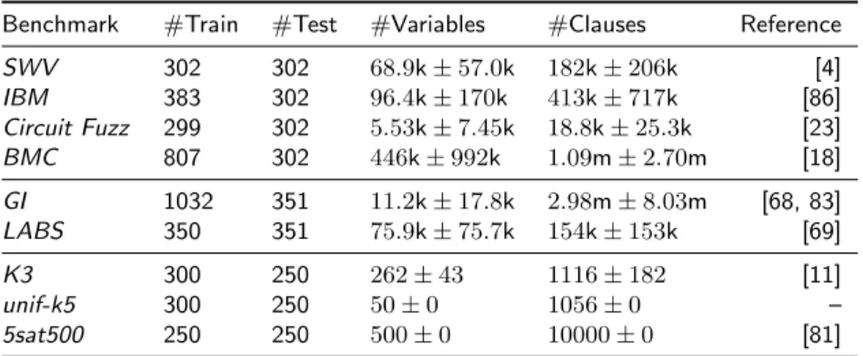
Table 1: Overview of benchmark sets used in the CSSC 2013 tracksIndustrial SAT+UNSAT,crafted SAT+UNSAT, andRandom SAT+UNSAT (from top to bottom); k and m stand for factors of one thousand and one million, respectively.
• ParamILS and SMAC have been shown to benefit substantially from multiple independent runs, since they are randomized algorithms. Givenk cores, the usual approach is simply to executekindependent configurator runs and pick the configuration from the one with best performance on the training set. GGA, on the other hand, can use multiple cores on a single machine, and in fact requires these to run effectively. Therefore, givenk available cores per configuration approach, we usedk independent runs of eachParamILS andSMAC, and one run using allk cores forGGA.
• GGAcould not handle the complex parameter conditionalities found in some solvers; for those solvers, we only ranParamILS andSMAC.
4. The Configurable SAT Solver Challenge 2013
The first CSSC4 was held in 2013. It featured three tracks mirroring those of the SAT competition: Industrial SAT+UNSAT,crafted SAT+UNSAT, and Random SAT+UNSAT. Table 1 lists the benchmark families we used in each of these tracks, all of which are described in detail in Appendix A. Within each track, we used the same number of test instances for each benchmark family, thereby weighting each equally in our analysis.
4.1. Participating Solvers and Their Parameters
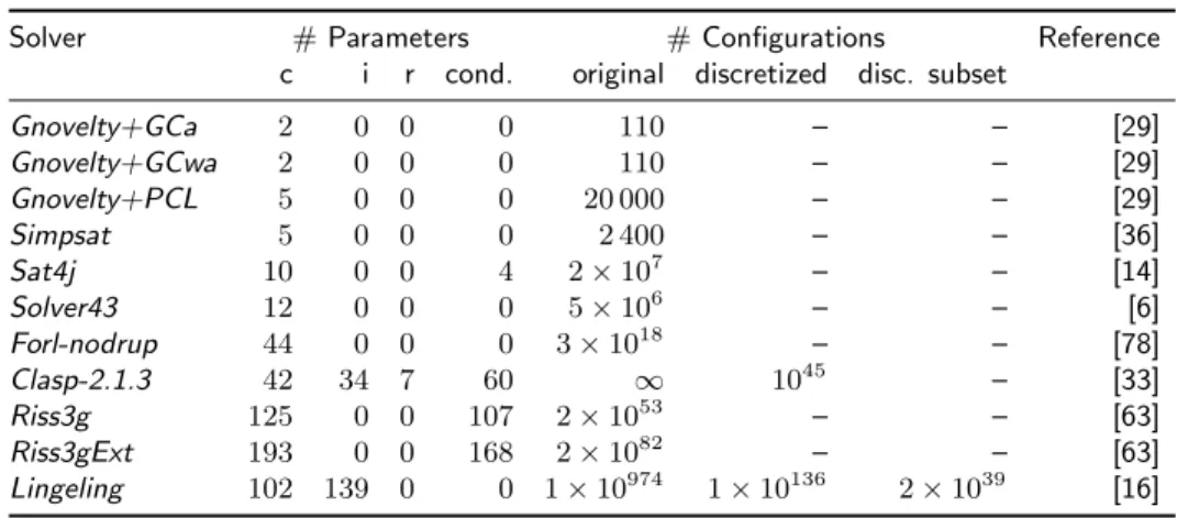
Table 2 summarizes the solvers that participated in the CSSC 2013, along with information on their configuration spaces. The eleven submitted solvers ranged from complete solvers based on conflict-directed clause learning (CDCL; [10]) to stochastic local search (SLS; [40]) solvers. The degree of parameterization
Solver # Parameters # Configurations Reference c i r cond. original discretized disc. subset
Gnovelty+GCa 2 0 0 0 110 – – [29]
Gnovelty+GCwa 2 0 0 0 110 – – [29]
Gnovelty+PCL 5 0 0 0 20 000 – – [29]
Simpsat 5 0 0 0 2 400 – – [36]
Sat4j 10 0 0 4 2×10⁷ – – [14]
Solver43 12 0 0 0 5×10⁶ – – [6]
Forl-nodrup 44 0 0 0 3×10¹⁸ – – [78]
Clasp-2.1.3 42 34 7 60 ∞ 1045 – [33]
Riss3g 125 0 0 107 2×1053 – – [63]
Riss3gExt 193 0 0 168 2×1082 – – [63]
Lingeling 102 139 0 0 1×10974 1×10136 2×1039 [16]
Table 2: Overview of solvers in the Configurable SAT Solver Challenge (CSSC) 2013 and their parameters of various types (‘c’ for categorical, ‘i’ for integer, ‘r’ for real-valued’); ‘cond’ identifies how many of these parameters are conditional. We also list the sizes of the configuration spaces provided by the solver developers (original, discretized, and the subset of the discrete parameters). Solvers are
ordered by the total number of parameters they expose (c+i+r).
varied substantially across these submitted solvers, from 2 to 241 parameters. We briefly discuss the main features of the solvers’ parameter configuration spaces, ordering solvers by their number of parameters.
Gnovelty+GCa andGnovelty+GCwa [29] are closely related SLS solvers. Both have two numerical parameters: the probability of selecting false clauses randomly and the probability of smoothing clause weights. The parameters were pre-discretized by the solver developer to 11 and 10 values, yielding 110 possible combinations.
Gnovelty+PCL[29] is an SLS solver with five parameters: one binary parameter (determining whether the stagnation path is dynamic or static) and four numerical parameters: the length of the stagnation path, the size of the time window storing stagnation paths, the probability of smoothing stagnation weights, and the probability of smoothing clause weights. All numerical parameters were pre-discretized to ten values each by the solver developer, yielding 20 000 possible combinations.
Simpsat[36] is a CDCL solver based onCryptominisat[77], which adds additional strategies for explicitly handling XOR constraints [37]. It has five numerical parameters that govern both these XOR constraint strategies and the frequency of random decisions. All parameters were pre-discretized by the solver developer, yielding 2 400 possible combinations.
Sat4j [14] is full-featured library of solvers for Boolean satisfiability and opti-mization problems. For the contest, it applied its default CDCL SAT solver with ten exposed parameters: four categorical parameters deciding between different restart strategies, phase selection strategies, simplifications, and cleaning; and six numerical parameters pre-discretized by its developer.
Solver43 [6] is a CDCL solver with 12 parameters: three categorical parameters concerning sorting heuristics used in bounded variable eliminiation, in definitions and in adding blocked clauses; and nine numerical parameters concerning various frequencies, factors, and limits. All parameters were pre-discretized by the solver developer.
Forl-nodrup [78] is a CDCL solver with 44 parameters. Most notably, these control variable selection, Boolean propagation, restarts, and learned clause removal. About a third of the parameters are numerical (particularly most of those concerning restarts and learned clause removal); all parameters were pre-discretized by the solver developer.
Clasp-2.1.3[33] is a solver for the more general answer set programming (ASP) problem, but it can also solve SAT, MAXSAT and PB problems. As a SAT solver, Clasp-2.1.3 is a CDCL solver with 83 parameters: 7 for pre-processing, 14 for the variable selection heuristic, 18 for the restart policy, 34 for the deletion policy, and 10 for a variety of other uses. The configuration space is highly conditional, with several top-level parameters enabling or disabling certain strategies. Clasp-2.1.3 exposes both a mixed continuous/discrete parameter configuration space and a manually-discretized one.
Riss3g [63] is a CDCL solver with 125 parameters. These include 6 numerical parameters from MiniSAT [30], 10 numerical parameters from Glucose [2], 17 mostly numerical Riss3G parameters, and 92 parameters controlling preprocess-ing/inprocessing performed by the integrated Coprocessor [62]. The inprocessor parameters resemble those inLingeling [16], emphasizing blocked clause elim-ination [51], bounded variable addition [65], and probing [61]. About 50 of the parameters are Boolean, and most others are numerical parameters pre-discretized by the solver developer. The parameter space is highly conditional, with inprocessor parameters dependent on a switch turning them on alongside various other dependencies. Indeed, there are only 18 unconditional parameters. Finally, there are also seven forbidden parameter combinations that ascertain various switches are turned on if inprocessing is used.
in Appendix C.
Lingeling[16] is a CDCL solver with 241 parameters (making it the solver with the largest configuration space in the CSSC 2013). 102 of these parameters are categorical, and the remaining 139 are integer-valued (76 of them with the trivial upper bound of max-integer, 231−1). Lingeling parameterizes many details of the solution process, including probing and look-ahead (about 25 mostly numerical parameters), blocked clause elimination and bounded variable elimination (about 20 mostly categorical parameters each), glue clauses (about 15 mostly numerical parameters), and a host of other mechanisms parameterized by about 5–10 parameters each. Lingeling exposes its full parameter space, a discretized version of all parameters, and a subspace of only the categorical parameters (102 of them).
4.2. Configuration Pipeline
We executed this competition on the QDR partition of the Compute Canada Westgrid cluster Orcinus. Each node in this cluster was provisioned with 24 GB memory and two 6-core, 2.66 GHz Intel Xeon X5650 CPUs with 12 MB L2 cache each, and ran Red Hat Enterprise Linux Server 5.5 (kernel 2.6.18, glibc 2.5).
In this first edition of the CSSC, we were unfortunately unable to runGGA. This was because it requires multiple cores for effective runtime minimization, and the respective multiple-core jobs we submitted on the Orcinus cluster were stuck in the queue for months without getting started. (Single-core runs, on the other hand, were often scheduled within minutes.)
We thus limited ourselves to usingParamILS for the discretized parameter space of each of the 11 solvers andSMAC for each of the parameter spaces that solver authors submitted (as discussed above, 9 submissions with one parameter space, 1 submission with two, and 1 submission with three, i.e., 14 in total). For each of the nine benchmark families, this gave rise to 11 configuration scenarios forParamILS and 14 forSMAC, for a total of 225 configuration scenarios. Since our budget for each configuration procedure was two CPU days on five cores (five independent runs ofParamILS andSMAC, respectively), the competition’s configuration phase required a total of 2250 CPU days (just over 6 CPU years). Thanks to a special allocation on the Orcinus cluster, we were able to complete this phase within a week.
Following standard practice, we then evaluated the configurations resulting from all configuration runs on the entire training data set and selected the configuration with the best training performance. We then executed only this configuration on the test set to assess the performance of the configured solver. This evaluation phase required much less time than the configuration phase.
We note that all scripts we used for performing the configuration and anal-ysis experiments were written in Ruby and are available for download on the competition website.
Rank Industrial SAT+UNSAT crafted SAT+UNSAT Random SAT+UNSAT
1st Lingeling Clasp-3.0.4-p8 Clasp-3.0.4-p8 2nd Riss3g Forl-nodrup Lingeling 3rd Solver43 Lingeling Riss3g
Table 3: Winners of the three tracks of CSSC 2013.
4.3. Results
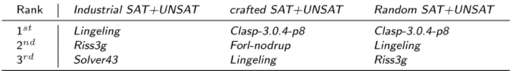
For each the three tracks of CSSC 2013, we configured each of the eleven submitted solvers for each of the benchmark families within the track and aggregated results across the respective test instances. We show the winners in Table 3 and discuss the results for each track in the following sections. Additional details, tables, and figures are provided in an accompanying technical report [43].
We remind the reader that the CSSC score only depends on how well the configured solver did andnot on the difference between default and configured performance. We nevertheless still cover default performance prominently in the following results, in order to emphasize the impact configuration had and the difference between the CSSC and standard solver competitions (e.g., the SAT competition).
4.3.1. Results of the Industrial SAT+UNSAT Track
Our Industrial SAT+UNSAT track consisted of the four industrial bench-marks detailed in Appendix A.1: Bounded Model Checking 2008 (BMC)[15], Circuit Fuzz [23],Hardware Verification (IBM) [86], andSWV [4].
Figure 1 visualizes the results of the configuration process for the winning solver Lingeling on these four benchmark sets. It demonstrates that even Lingeling, a highly competitive solver in terms of default performance, can be configured for improved performance on a wide range of benchmarks. We note that for the easy benchmarkSWV, configuration sped upLingelingby a factor of 20 (average runtime 3.3svs0.16s), and that for the harderCircuit Fuzz instances, it nearly halved the number of timeouts (39vs 20). The improvements were smaller for more traditional hardware verification instances (IBM andBMC) similar to those used to determineLingeling’s default parameter settings.
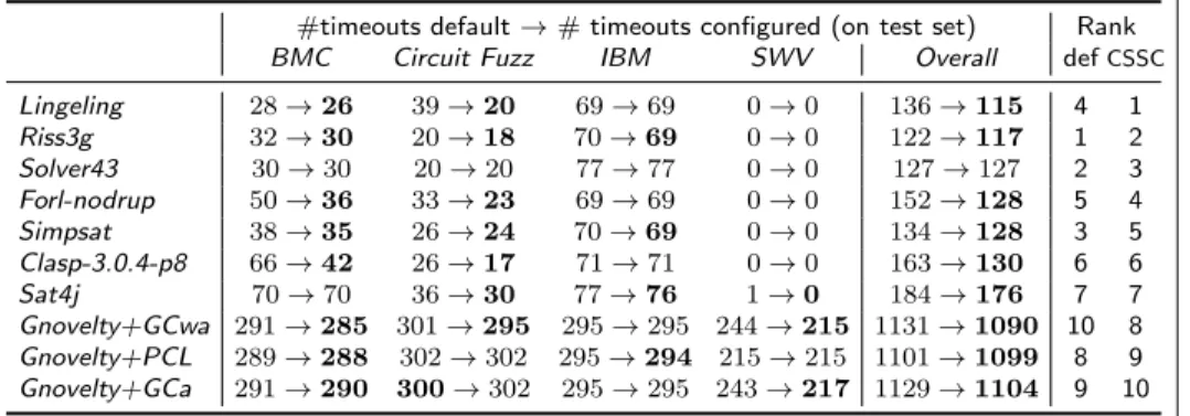
Table 4 summarizes the results of the ten solvers that were eligible for medals. From this table, we note that, like Lingeling, many other solvers benefited from configuration. Indeed, some solvers (in particularForl-nodrupand Clasp-3.0.4-p8) benefited much more from configuration on theBMC instances, largely because their default performance was worse on this benchmark. On the other hand,Riss3g featured stronger default performance thanLingeling but did not benefit as much from configuration.
Results for CSSC 2013 Industrial SAT+UNSAT track
10−2 10−1 1 10 100
Default in sec.
10−2 10−1 1 10 100
Configured in sec.
2x 2x 10x 10x 100x 100x 300 300 timeout timeout (a)BMC
PAR-10: 302→282
10−2 10−1 1 10 100
Default in sec.
10−2 10−1 1 10 100
Configured in sec.
2x 2x 10x 10x 100x 100x 300 300 timeout timeout
(b)Circuit Fuzz PAR-10: 409→241
10−2 10−1 1 10 100
Default in sec.
10−2 10−1 1 10 100
Configured in sec.
2x 2x 10x 10x 100x 100x 300 300 timeout timeout (c)IBM
PAR-10: 694→692
10−2 10−1 1 10 100
Default in sec.
10−2 10−1 1 10 100
Configured in sec.
2x 2x 10x 10x 100x 100x 300 300 timeout timeout (d)SWV
PAR-10: 3.32→0.16
Figure 1: Speedups achieved by configuration ofLingeling. For each benchmark, we show scatter plots of solver defaults vs. configured parameter settings.
#timeouts default→#timeouts configured (on test set) Rank
BMC Circuit Fuzz IBM SWV Overall defCSSC
Lingeling 28→26 39→20 69→69 0→0 136→115 4 1
Riss3g 32→30 20→18 70→69 0→0 122→117 1 2
Solver43 30→30 20→20 77→77 0→0 127→127 2 3
Forl-nodrup 50→36 33→23 69→69 0→0 152→128 5 4
Simpsat 38→35 26→24 70→69 0→0 134→128 3 5
Clasp-3.0.4-p8 66→42 26→17 71→71 0→0 163→130 6 6
Sat4j 70→70 36→30 77→76 1→0 184→176 7 7
Gnovelty+GCwa 291→285 301→295 295→295 244→215 1131→1090 10 8
Gnovelty+PCL 289→288 302→302 295→294 215→215 1101→1099 8 9
Gnovelty+GCa 291→290 300→302 295→295 243→217 1129→1104 9 10
Table 4: Results for CSSC 2013 competition trackIndustrial SAT+UNSAT. For each solver and benchmark, we show the number of test set timeouts achieved with the default and the configured parameter setting, bold-facing the better one; we broke ties by the solver’s average runtime (not shown for brevity). We aggregated results across all benchmarks to compute the final ranking.
Results for CSSC 2013crafted SAT+UNSAT track
10−2 10−1 1 10 100 Default in sec.
10−2
10−1
1 10 100
Configured in sec.
2x
2x
10x
10x
100x
100x
300
300
timeout
timeout
(a)Graph Isomorphism (GI) PAR-10: 362→65
10−2 10−1 1 10 100 Default in sec.
10−2
10−1
1 10 100
Configured in sec.
2x
2x
10x
10x
100x
100x
300
300
timeout
timeout
(b)Low Autocorrelation Binary Sequence (LABS).
PAR-10: 837→779
Figure 2: Speedups achieved by configuration ofClasp-3.0.4-p8 on the CSSC 2013crafted SAT+UNSAT track. We show scatter plots of default vs. config-ured versions ofClasp-3.0.4-p8.
#TOs default→#TOs configured (on test set) Rank
GI LABS Overall def CSSC
Clasp-3.0.4-p8 42→6 97→90 139→96 2 1
Forl-nodrup 40→7 95→91 135→98 1 2
Lingeling 43→10 105→97 148→107 3 3
Riss3g 51→42 97→89 148→131 4 4
Simpsat 42→42 107→107 149→149 5 5
Solver43 66→65 90→87 156→152 6 6
Sat4j 62→57 110→104 172→161 7 7
Gnovelty+GCwa 180→180 195→154 375→334 8 8 Gnovelty+GCa 183→180 240→173 423→353 10 9 Gnovelty+PCL 179→178 199→183 378→361 9 10
Table 5: Results for CSSC 2013 competition track crafted SAT+UNSAT. For each solver and benchmark, we show the number of test set timeouts achieved with the default and the configured parameter setting, bold-facing the better one. We aggregated results across all benchmarks to compute the final ranking.
on default performance, the overall winning solver,Lingeling, would have only ranked fourth.
4.3.2. Results of the crafted SAT+UNSAT Track
Binary Sequence (LABS).
Figure 2 visualizes the improvements algorithm configuration yielded for the best-performing solverClasp-3.0.4-p8 on these benchmarks. Improvements were particularly large on theGI instances, where algorithm configuration decreased the number of timeouts from 42 to 6. Table 5 summarizes the results we obtained for all solvers on these benchmarks, showing that configuration also substantially improved the performance of many other solvers. The table also aggregates results across both benchmark families to yield overall results for thecrafted SAT+UNSAT track. WhileForl-nodrupshowed the best default performance and benefited substantially from configuration (#timeouts reduced from 135 to 98),Clasp-3.0.4-p8 improved even more (#timeouts reduced from 139 to 96).
4.3.3. Results of the Random SAT+UNSAT Track
The Random SAT+UNSAT track consisted of three random benchmarks detailed in Appendix A.3: 5sat500,K3, andunif-k5. The instances in5sat500 were all satisfiable, those inunif-k5 all unsatisfiable, and those inK3 were mixed.
Table 6 summarizes the results for these benchmarks. It shows that the unif-k5benchmark set was very easy for complete solvers (although configuration still yielded up to 4-fold speedups), that theK3 benchmark was also quite easy for the best solvers, and that only the SLS solvers could tackle benchmark 5sat500, with configuration making a big difference to performance.
Here again, our aggregate results demonstrate that rankings were substantially different between the default and configured versions of the solvers: the three solvers with top default performance were ranked 4th to 6th in the CSSC, and vice versa. Figure 3 visualizes the very substantial speedups achieved by configuration for the winning solverClasp-3.0.4-p8 onK3 andunif-k5, and for the SLS solverGnovelty+GCa on5sat500.
5. The Configurable SAT Solver Challenge 2014
The second CSSC5 was held in 2014. Compared to the inaugural CSSC in 2013, we improved the competition design in several ways:
• We used a different computer cluster,6 enabling us to runGGAas one of the configuration procedures.
• We added a Random SAT track to facilitate comparisons of stochastic local search solvers.
• We dropped the (too easy) SWV benchmark family and introduced four new benchmark families, yielding a total of three benchmark families in each of the four tracks, summarized in Table 7 and described in detail in Appendix A.
5http://aclib.net/cssc2014/
6We executed this competition on the META cluster at the University of Freiburg, whose
compute nodes contained 64GB of RAM and two 2.60GHz Intel Xeon E5-2650v2 8-core CPUs with 20 MB L2 cache each, running Ubuntu 14.04 LTS, 64bit.
Results for CSSC 2013Random SAT+UNSAT track
10−2 10−1 1 10 100 Default in sec. 10−2
10−1 1 10 100
Configured in sec.
2x 2x 10x 10x 100x 100x 300 300 timeout timeout (a)Gnovelty+GCaon
5sat500
PAR-10: 1997→77
10−2 10−1 1 10 100 Default in sec. 10−2
10−1 1 10 100
Configured in sec.
2x 2x 10x 10x 100x 100x 300 300 timeout timeout (b)Clasp-3.0.4-p8 onK3
PAR-10: 158→2.79
10−2 10−1 1 10 100 Default in sec. 10−2
10−1 1 10 100
Configured in sec.
2x 2x 10x 10x 100x 100x 300 300 timeout timeout (c)Clasp-3.0.4-p8onunif-k5
PAR-10: 1.44→0.37
Figure 3: Speedups achieved by configuration on the CSSC 2013 Random SAT+UNSAT track. We show scatter plots of default vs. configured solvers..
#TOs default→#TOs configured (on test set) Rank
5sat500 K3 unif-k5 Overall def CSSC
Clasp-3.0.4-p8 250→250 11→0 0→0 261→250 6 1
Lingeling 250→250 8→0 0→0 258→250 4 2
Riss3g 250→250 10→0 0→0 260→250 5 3
Solver43 250→250 6→3 0→0 256→253 2 4
Simpsat 250→250 4→4 0→0 254→254 1 5
Sat4j 250→250 7→5 0→0 257→255 3 6
Forl-nodrup 250→250 39→8 0→0 289→258 7 7
Gnovelty+GCwa 8→1 124→124 250→250 382→375 8 8
Gnovelty+GCa 163→4 124→124 250→250 537→378 9 9
Gnovelty+PCL 250→11 124→124 250→250 624→385 10 10
Table 6: Results for CSSC 2013 competition trackRandom SAT+UNSAT. For each solver and benchmark, we show the number of test set timeouts achieved with the default and the configured parameter setting, bold-facing the better one. Results were aggregated across all benchmarks to compute the final ranking. We broke ties by the solver’s average runtime. While we do not show runtimes for brevity, the runtimes important for the ranking were the average runtimes of the top 3 solvers on the union of K3 andunif-k5: 1.58s (Clasp-3.0.4-p8), 4.20s (Lingeling), and 7.68s (Riss3g).
• We let solver authors decide which tracks their solver should run in.
• For fairness, for each solver, we performed the same number of configuration experiments. (This is in contrast to 2013, where we performed the same number of configuration runsfor every configuration space of every solver, which lead to a larger combined configuration budget for solvers submitted with multiple configuration spaces).
Benchmark #Train #Test #Variables #Clauses Reference
IBM 383 302 96.4k±170k 413k±717k [86] Circuit Fuzz 299 302 5.53k±7.45k 18.8k±25.3k [23] BMC 604 302 424k±843k 1.03m±2.30m [18]
GI 1032 351 11.2k±17.8k 2.98m±8.03m [68, 83] LABS 350 351 75.9k±75.7k 154k±153k [69] N-Rooks 484 351 38.2k±37.4k 125k±126k [67]
K3 300 250 262±43 1116±182 [11]
3cnf 500 250 350±0 1493±0 [12]
unif-k5 300 250 50±0 1056±0 –
3sat1k 250 250 500±0 10000±0 [81]
5sat500 250 250 1000±0 4260±0 [81]
7sat90 250 250 90±0 7650±0 [81]
Table 7: Overview of benchmark sets used in the CSSC 2014 tracksIndustrial SAT+UNSAT, crafted SAT+UNSAT, Random SAT+UNSAT, and Random SAT (from top to bottom); k and m stand for factors of one thousand and one million, respectively.
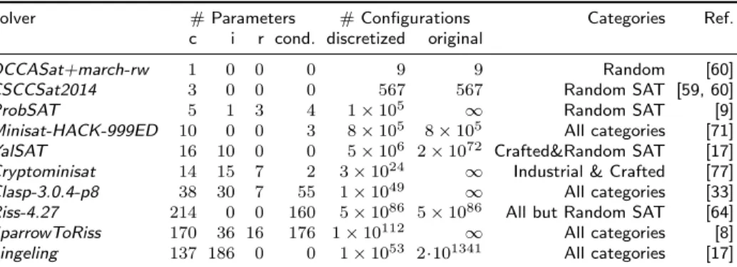
Solver # Parameters # Configurations Categories Ref.
c i r cond. discretized original
DCCASat+march-rw 1 0 0 0 9 9 Random [60]
CSCCSat2014 3 0 0 0 567 567 Random SAT [59, 60]
ProbSAT 5 1 3 4 1×10⁵ ∞ Random SAT [9]
Minisat-HACK-999ED 10 0 0 3 8×10⁵ 8×10⁵ All categories [71]
YalSAT 16 10 0 0 5×10⁶ 2×1072 Crafted&Random SAT [17]
Cryptominisat 14 15 7 2 3×1024 ∞ Industrial & Crafted [77]
Clasp-3.0.4-p8 38 30 7 55 1×1049 ∞ All categories [33]
Riss-4.27 214 0 0 160 5×1086 5×1086 All but Random SAT [64]
SparrowToRiss 170 36 16 176 1×10112 ∞ All categories [8]
Lingeling 137 186 0 0 1×1053 2·101341 All categories [17]
Table 8: Overview of solvers in the CSSC 2014 and their parameters of various types (‘c’ for categorical, ‘i’ for integer, ‘r’ for real-valued’); ‘cond’ identifies how many of these parameters are conditional. For each solver, we also list the sizes of the original configuration space submitted by solver developers and of a discretized version, as well as the categories in which the solver participated. Solvers are ordered by the number of parameters they expose (c+i+r).
configuration process and made all information about errors available to solver developers after the competition.
5.1. Participating Solvers
The ten solvers that participated in the CSSC 2014 are summarized in Table 8; they included CDCL, SLS and hybrid solvers. These solvers differed substantially in their degree of parameterization, with the number of parameters ranging
from 1 to 323. We briefly discuss the main features of each solver’s parameter configuration space, ordering solvers by their number of parameters.
DCCASat+march-rw[60] combines the SLS solver DCCASat with the CDCL solver march-rw. It was submitted to theRandom SAT+UNSAT track. Its only (continuous) parameter is the time ratio of the SLS solver. This parameter was
pre-discretized to nine values.
CSCCSat2014 [59, 60] is an SLS solver based on configuration checking and dynamic local search methods. It was submitted to the Random SAT track. It features 3 continuous parameters that were pre-discretized to 7, 9, and 9 values each, giving rise to a total configuration space of 567 possible parameter configurations. The parameters control the weighting of the dynamic local search part and the probabilities for the linear make functions used in the random walk steps.
ProbSAT [9] is a simple SLS solver based on probability distributions that are built from simple features, such as the make and break of variables [9]. ProbSAT’s 9 parameters control the type and the parameters of the probability distribution, as well as the type of restart. ProbSAT was submitted to the Random SAT track.
Minisat-HACK-999ED [71] is a CDCL solver; it was submitted to all tracks. It has one categorical parameter (whether or not to use the Luby restarting strategy) and 9 numerical parameters fine-tuning the Luby and geometric restart strategies, as well as controlling clause removal and the treatment of glue clauses. 3 of these 9 numerical parameters are conditional on the choice of the Luby restart strategy, and all numerical parameters were pre-discretized by the solver developer. There are also 3 forbidden parameter combinations derived from a weak inequality constraint between two parameter values.
YalSAT [17] is an SLS solver; it was submitted to the trackscrafted SAT+UNSAT andRandom SAT. It has 27 parameters that parameterize the solver’s restart component (7 parameters) amongst many other components. 11 of the 27 parameters are numerical, with 6 of them having a trivial upper bound of max-integer (231−1).
Cryptominisat [77] is a CDCL solver; it was submitted to the tracks Industrial SAT+UNSAT and crafted SAT+UNSAT. It has 29 parameters that control restarts (6 mostly numerical parameters), clause removal (7 mostly numerical parameters), variable branching and polarity (3 parameters each), simplification (5 parameters), and several other mechanisms. 2 of the numerical parameters further parameterize the blocking restart mechanism and are thus conditional on that mechanism being selected.
(ASP) problem, but it can also solve SAT, MAXSAT and PB problems. It is fundamentally similar to the solver submitted in 2013; changes in the new version focused on the ASP solving part rather than the SAT solving part. As a SAT solver,Clasp-3.0.4-p8 has 75 parameters, of which 7 control preprocessing, 14 variable selection, 19 the restart policy, 28 the deletion policy and 7 miscellaneous other mechanisms. The configuration space is highly conditional, with several top-level parameters enabling or disabling certain strategies. Finally, there are also 2 forbidden parameter combinations that prevent certain combinations of deletion strategies. Clasp-3.0.4-p8 exposes both a mixed continuous/discrete parameter configuration space and a manually-discretized one. It was submitted to all tracks.
Riss-4.27 [64] is a CDCL solver submitted to all tracks except Random SAT. Compared to the 2013 versionRiss3g, it almost doubled its number of param-eters, yielding 214 parameters organized into 121 simplification and 93 search parameters. In particular, it added many new preprocessing and inprocessing techniques, including XOR handling (via Gaussian elimination [37]), and extract-ing cardinality constraints [20]. Roughly half of the simplification parameters and a third of the search parameters are categorical (in both cases most of the categoricals are binary). The simplification parameters comprise about 20 Boolean switches for preprocessing techniques and about 100 in-processor parameters, prominently including blocked clause elimination, bounded variable addition, equivalance elimination [34], numerical limits, probing, symmetry break-ing, unhiding [39], Gaussian elimination, covered literal elimination [66], and even some stochastic local search. The search parameters parameterize a wide range of mechanisms including variable selection, clause learning and removal, restarts, clause minimization, restricted extended resolution, and interleaved clause strengthening.
SparrowToRiss [8] combines the SLS solver Sparrow with the CDCL solver Riss-4.27 by first running Sparrow, followed by Riss-4.27. It was submitted to all tracks. SparrowToRiss’s configuration space is that of Riss-4.27 plus 6 Sparrow parameters and 2 parameters controlling when to switch fromSparrow toRiss-4.27: the maximal number of flips forSparrow (by default 500 million) and the CPU time forSparrow (by default 150 seconds). Also, in contrast to Riss-4.27,SparrowToRiss does not pre-discretize its numerical parameters, but expresses them as 36 integer and 16 continuous parameters.
Lingeling [17] is a successor to the 2013 version; it was submitted to the tracks Industrial SAT+UNSAT andcrafted SAT+UNSAT. Compared to 2013, Lin-geling’s parameter space grew by roughly a third, to a total of 323 parameters (meaning that again,Lingeling was the solver with the most parameters). As in 2013, roughly 40% of these parameters were categorical and the rest integer-valued (many with a trivial upper bound of max-integer, 231−1). Notable groups of parameters that were introduced in the 2014 version include additional preprocessing/inprocessing options and new restart strategies.
Rank Industrial SAT+UNSAT crafted SAT+UNSAT Random SAT+UNSAT Random SAT
1st Lingeling Clasp-3.0.4-p8 Clasp-3.0.4-p8 ProbSAT 2nd Minisat-HACK-999ED Lingeling DCCASat+march-rw SparrowToRiss 3rd Clasp-3.0.4-p8 Cryptominisat Minisat-HACK-999ED CSCCSat2014
Table 9: Winners of the four tracks of CSSC 2014.
5.2. Configuration Pipeline
In the CSSC 2014, we used the configuratorsParamILS,GGA, andSMAC. For each benchmark and solver, we ranGGA andSMAC on the solver’s full configuration space, which could contain an arbitrary combination of numerical and categorical parameters. We also ran all configurators on a discretized version of the configuration space (automatically constructed unless provided by the solver authors), yielding a total of five configuration approaches: ParamILS -discretized,GGA,GGA-discretized,SMAC, andSMAC-discretized. GGAcould not handle the complex conditionals of some solvers; therefore, for these solvers we only ran ParamILS and the twoSMAC variants.
Due to the cost of running a third configurator on nearly every configuration scenario, we reduced the budget for each configuration approach from two CPU days on five cores in CSCC 2013 to two CPU days on four cores in CSSC 2014. In the case ofParamILS andSMAC, as in 2013, we used these four cores to perform four independent 2-day configurator runs. In the case ofGGA, we performed one 2-day run using all four cores. We evaluated the configurations resulting from each of the 14 configuration runs (4ParamILS-discretized, 4SMAC-discretized, 4SMAC, 1 GGA-discretized, and 1GGA) on the entire training data set of the benchmark at hand and selected the configuration with the best performance. We then executed only this configuration on the benchmark’s test set to determine the performance of the configured solver.
In the four tracks of the CSSC (Industrial SAT+UNSAT,crafted SAT+UNSAT, Random SAT+UNSAT,Random SAT) we had 6, 6, 5, and 6 participating solvers, respectively, and since there were three benchmark families per track, we ended up with (6 + 6 + 5 + 6)×3 = 72 pairs of solvers and benchmarks to configure them on. For each of these configuration scenarios, each of the 5 configuration approaches above required four cores for 2 days, yielding a total computational expense of 72×5×4×2 = 2880 CPU days (close to 8 CPU years). Thanks to a special allocation on the META cluster at the University of Freiburg, we were able to finish this process within 2 weeks.
We note that all scripts we used for performing the configuration and analysis experiments were written in Python (updated from Ruby in 2013) and are available for download on the competition website.
5.3. Results
Results for CSSC 2014Industrial SAT+UNSAT track
10−2 10−1 1 10 100 Default in sec. 10−2
10−1 1 10 100
Configured in sec.
2x 2x 10x 10x 100x 100x 300 300 timeout timeout (a)BMC PAR-10: 222→221
10−2 10−1 1 10 100 Default in sec. 10−2
10−1 1 10 100
Configured in sec.
2x 2x 10x 10x 100x 100x 300 300 timeout timeout (b)Circuit Fuzz PAR-10: 316→193
10−2 10−1 1 10 100 Default in sec. 10−2
10−1 1 10 100
Configured in sec.
2x 2x 10x 10x 100x 100x 300 300 timeout timeout (c)IBM
PAR-10: 697→694
Figure 4: Scatter plots of default vs. configuredLingeling, the gold-medal winner of theIndustrial SAT+UNSAT track of CSSC 2014.
#timeouts default→#timeouts configured (on test set) Rank
BMC Circuit Fuzz IBM Overall def CSSC
Lingeling 20→20 30→18 69→69 119→107 2 1
Minisat-HACK-999ED 22→22 21→19 70→70 113→111 1 2
Clasp-3.0.4-p8 44→30 18→12 71→71 133→113 4 3
Riss-4.27 39→26 20→22 72→72 131→120 3 4
Cryptominisat 40→37 31→20 70→69 141→126 5 5
SparrowToRiss 62→36 29→21 72→72 163→129 6 6
Table 10: Results for CSSC 2014 competition track Industrial SAT+UNSAT. For each solver and benchmark, we show the number of test set timeouts achieved with the default and the configured parameter setting, bold-facing the better one. We aggregated results across all benchmarks to compute the final ranking.
each track in Table 9 and discuss the results in the following sections. Additional details, tables, and figures are provided in an accompanying technical report [48].
5.3.1. Results of the Industrial SAT+UNSAT Track
TheIndustrial SAT+UNSAT track consisted of three industrial benchmarks detailed in Appendix A.1: BMC [15],Circuit Fuzz [23], andIBM [86]. Figure 4 visualizes the results of applying algorithm configuration to the winning solverLingeling on these three benchmark sets. It shows similar results as in the Industrial SAT+UNSAT track of CSSC 2013: Lingeling’s strong default performance on ‘typical’ hardware verification benchmarks (IBM and BMC) could only be improved slightly by configuration, but much larger improvements were possible on less standard benchmarks, such asCircuit Fuzz.
Table 10 summarizes the results for all six solvers that participated in the Industrial SAT+UNSAT track. These results demonstrate that, in contrast to Lingeling, several solvers (in particular,Clasp-3.0.4-p8,Riss-4.27, and
Results for CSSC 2014crafted SAT+UNSAT track
10−2 10−1 1 10 100 Default in sec. 10−2
10−1 1 10 100
Configured in sec.
2x 2x 10x 10x 100x 100x 300 300 timeout timeout (a)GI
PAR-10: 370→90
10−2 10−1 1 10 100 Default in sec. 10−2
10−1 1 10 100
Configured in sec.
2x 2x 10x 10x 100x 100x 300 300 timeout timeout (b)LABS PAR-10: 755→804
10−2 10−1 1 10 100 Default in sec. 10−2
10−1 1 10 100
Configured in sec.
2x 2x 10x 10x 100x 100x 300 300 timeout timeout (c)N-Rooks PAR-10: 705→5
Figure 5: Scatter plots of default vs. configured Clasp-3.0.4-p8, the gold medal winner of thecrafted SAT+UNSAT track of CSSC 2014.
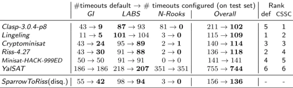
#timeouts default→#timeouts configured (on test set) Rank
GI LABS N-Rooks Overall def CSSC
Clasp-3.0.4-p8 43→9 87→93 81→0 211→102 5 1
Lingeling 11→5 101→104 3→0 115→109 1 2
Cryptominisat 43→24 95→89 2→1 140→114 3 3
Riss-4.27 43→30 91→88 2→0 136→118 2 4
Minisat-HACK-999ED 50→50 91→91 0→0 141→141 4 5
YalSAT 186→186 218→207 351→351 755→744 6 6
SparrowToRiss(disq.) 55→42 98→94 3→0 156→136 -
-Table 11: Results for CSSC 2014 competition track crafted SAT+UNSAT. For each solver and benchmark, we show the number of test set timeouts achieved with the default and the configured parameter settings, bold-facing the better one. We aggregated results across all benchmarks to compute the final ranking. SparrowToRiss was disqualified from this track, since it returned ‘satisfiable’ for one instance without producing a model.
ToRiss) benefited largely from configuration on the BMC benchmark, but did not reachLingeling’s performance even after configuration. Minisat-HACK-999ED performed even better thanLingeling with its default parameters, but did not benefit from configuration as much asLingeling(particularly on theCircuit Fuzz benchmark family).
5.3.2. Results of the crafted SAT+UNSAT Track
it reduced the number of timeouts from 81 to 0. Similar to the results from CSSC 2013, configuration also substantially improved performance on theGI instances, decreasing the number of timeouts from 43 to 9. In contrast to 2013, an unusual effect occurred forClasp-3.0.4-p8 on theLABS instances, where the number of timeouts on the test setincreased from 87 to 93 by configuration; we study the reasons for this in more detail in Section 6.1.
Table 11 summarizes the results of all solvers on thecrafted SAT+UNSAT track, showing that the performance of many other solvers also substantially improved on the benchmarksGI andN-Rooks, and only mildly (if at all) on the LABS benchmark. The aggregate results across these 3 benchmark families show thatLingeling had the best default performance, but only benefited mildly from configuration (#timeouts reduced from 115 to 109), whereas Clasp-3.0.4-p8 benefited much more from configuration and thus outperformedLingeling af-ter configuration (#timeouts reduced from 211 to 102). Once again, we note that the winning solver only showed mediocre performance based on its de-fault: Clasp-3.0.4-p8 would have ranked 5th in a comparison based on default performance.
5.3.3. Results of the Random SAT+UNSAT Track
The Random SAT+UNSAT track consisted of three random benchmarks detailed in Appendix A.3: 3cnf,K3, andunif-k5. The instances inunif-k5 are all unsatisfiable, while the other two sets contain both satisfiable and unsatisfiable instances. Figure 6 visualizes the improvements achieved by configuration on these benchmarks for the best-performing solverClasp-3.0.4-p8. Clasp-3.0.4-p8 benefited most from configuration on benchmark 3cnf, where it reduced the number of timeouts from 18 to 0. For the other benchmarks, it could already solve all instances in its default parameter configuration, but configuration helped reduce its average runtime by factors of 3 (K3) and 2 (unif-k5), respectively. Table 12 summarizes the results of all solvers for these benchmarks. We note that solverDCCASat+march-rw showed the best default performance, and that after configuration, it also solved all instances from the three benchmark sets, only ranking behindClasp-3.0.4-p8 because the latter solved these instances faster.
5.3.4. Results of the Random SAT Track
The Random SAT track consisted of the three benchmarks detailed in Appendix A.3: 3sat1k,5sat500 and7sat90. Figure 7 visualizes the improvements configuration achieved on these benchmarks for the best-performing solver ProbSAT.ProbSAT benefited most from configuration on benchmark 5sat500: its default did not solve a single instance in the maximum runtime of 300 seconds, while its configured version solved all instances in an average runtime below 2 seconds! Since timeouts at 300s yield a PAR-10 score of 3000, the PAR-10 speedup factor on this benchmark was 1 500, the largest we observed in the CSSC. On the other two scenarios, configuration was also very beneficial, reducingProbSAT’s number of timeouts from 24 to 0 (7sat90) and from 10 to 4 (3sat1k), respectively. Table 13 summarizes the results of all solvers for these benchmarks, showing that
Results for CSSC 2014 Random SAT+UNSAT track
10−2 10−1 1 10 100 Default in sec. 10−2
10−1 1 10 100
Configured in sec.
2x 2x 10x 10x 100x 100x 300 300 timeout timeout (a)3cnf
PAR-10: 309→35
10−2 10−1 1 10 100 Default in sec. 10−2
10−1 1 10 100
Configured in sec.
2x 2x 10x 10x 100x 100x 300 300 timeout timeout (b)K3
PAR-10: 7.91→2.66
10−2 10−1 1 10 100 Default in sec. 10−2
10−1 1 10 100
Configured in sec.
2x 2x 10x 10x 100x 100x 300 300 timeout timeout (c)unif-k5 PAR-10: 0.74→0.30
Figure 6: Scatter plots of default vs. configured Clasp-3.0.4-p8, the gold medal winner of theRandom SAT+UNSAT track of CSSC 2014.
#timeouts default→#timeouts configured (on test set) Rank
3cnf K3 unif-k5 Overall def CSSC
Clasp-3.0.4-p8 18→0 0→0 0→0 18→0 2 1
DCCASat+march-rw 1→0 0→0 1→0 2→0 1 2
Minisat-HACK-999ED 166→99 5→1 0→0 171→100 5 3
Riss-4.27 160→113 2→2 1→0 163→115 4 4
SparrowToRiss 126→126 8→1 0→0 134→127 3 5
Table 12: Results for CSSC 2014 competition trackRandom SAT+UNSAT. For each solver and benchmark, we show the number of test set timeouts achieved with the default and the configured parameter settings, bold-facing the better one; we broke ties by the solver’s average runtime (not shown for brevity, but the average runtimes important for tie breaking were 13 seconds for configured Clasp-3.0.4-p8 and 21 seconds for config-uredDCCASat+march-rw). We aggregated results across all benchmarks to compute the final ranking.
next toProbSAT, onlySparrowToRiss benefited from configuration. Neither of the CDCL solvers (Clasp-3.0.4-p8 andMinisat-HACK-999ED) solved a single instance in any of the three benchmarks (in either default or configured variants). For the other two SLS solvers,YalSAT andCSCCSat2014, the defaults were already well tuned for these benchmark sets. Indeed, we observed overtuning to the training sets in one case each: YalSAT for3sat1k andCSCCSat2014 for 7sat90. Overall, the configurability ofProbSAT andSparrowToRissallowed them to place first and second, respectively, despite their poor default performance (especially on5sat500, where neither of them solved a single instance with default
Results for CSSC 2014Random SAT track
10−2 10−1 1 10 100 Default in sec. 10−2
10−1 1 10 100
Configured in sec.
2x 2x 10x 10x 100x 100x 300 300 timeout timeout (a)3sat1k PAR-10: 132→53
10−2 10−1 1 10 100 Default in sec. 10−2
10−1 1 10 100
Configured in sec.
2x 2x 10x 10x 100x 100x 300 300 timeout timeout (b)5sat500 PAR-10: 3000→2
10−2 10−1 1 10 100 Default in sec. 10−2
10−1 1 10 100
Configured in sec.
2x 2x 10x 10x 100x 100x 300 300 timeout timeout (c)7sat90 PAR-10: 337→15
Figure 7: Scatter plots of default vs. configured ProbSAT, the gold medal winner of theRandom SAT track of CSSC 2014.
#timeouts default→#timeouts configured (on test set) Rank
3sat1k 5sat500 7sat90 Overall def CSSC
ProbSAT 10→4 250→0 24→0 284→4 4 1
SparrowToRiss 9→5 250→0 3→3 262→8 3 2
CSCCSat2014 2→2 0→0 3→6 5→8 1 3
YalSAT 6→7 0→0 5→5 11→12 2 4
Clasp-3.0.4-p8 250→250 250→250 250→250 750→750 5 5
Minisat-HACK-999ED 250→250 250→250 250→250 750→750 6 6
Table 13: Results for CSSC 2014 competition track Random SAT. For each solver and benchmark, we show the number of test set timeouts achieved with the default and the configured parameter settings, bold-facing the better one; we broke ties by the solver’s average runtime (not shown for brevity). We aggregated results across all benchmarks to compute the final ranking.
6. Post-Competition Analyses
While the previous sections focussed on the results of the respective com-petitions, we now discuss several analyses we performed afterwards to study overarching phenomena and general patterns.
6.1. Why Does Configuration Work So Well and How Can It Fail?
Several practitioners have asked us why automated configuration can yield the large speedups over the default configuration we observed. We believe there are two key reasons for this:
• No single algorithmic approach performs best on all types of benchmark instances; this is precisely the same reason that algorithm selection ap-proaches (such as SATzilla [85] or 3S [52]) work so well.
(a)N-Rooks (b)LABS
Figure 8: Trainingvs test PAR-10 scores of 100 randomClasp configurations and theClasp-3.0.4-p8 default.
• Solver defaults are typically chosen to be robust across benchmark fam-ilies. For any given benchmark family F, highly parameterized solvers can, however, typically be instantiated to exploit the idiosyncrasies ofF substantially better. (These improvements only need to generalize to other instances fromF, not to other benchmark families.)
However, algorithm configuration does not necessarily work in all cases. For example, in thecrafted SAT+UNSAT track of the CSSC 2014, we encountered a case in which the configured solver performed somewhatworse than the default solver: Clasp configured on benchmark family LABS timed out on 93 test instances, whereas its default only timed out on 87 test instances (see also Figure 5b). Two obvious causes suggest themselves in the case of such a failure:
• insufficiently long configuration runs (which can result in worse-than-default performance on thetraining set7); and/or
• overtuning on the training set that does not generalize to thetest set.
We investigated the configuration ofClasponLABSfurther after the competition, and found that in this caseboth of these effects applied: In the CSSC, training performance slightly deteriorated (86→87 timeouts); and the improved training performance we found with a larger configuration budget8 afterwards (86→83 timeouts) also did not generalize to the test set (87→88 timeouts).
To contrast the conditions under which configuration can fail and under which it works well, we compared the configuration of Clasp on benchmarks
7Worse-than-default performance on the training set is possible since configurators only base their decisions on asubset of the training instances; that subset increases over time and only reaches the full training set when the configuration process is given enough time.
LABS (87→93 test timeouts in the CSSC) andN-Rooks (81→0 test timeouts in the CSSC). For this analysis, we sampled 100Clasp configurations uniformly at random and evaluated their PAR-10 training and test scores on both of the benchmarks; Figure 8 shows the result. The first observation we make directly based on the figure is that for N-Rooks, about 20% of the random configurations outperform the default, whereas forLABS none of them do: the default is simply very good to start with forLABS and thus much harder to beat. Second, since several configurations are very good (i.e., fast) forN-Rooks, configurators can make progress much faster (and also take full advantage of adaptive capping to limit the time spent with poor configurations); indeed, in the CSSC the configurators managed to perform about 8 times moreClasp runs in the same time (2 days) forN-Rooks than forLABS (averaging about 14 400 vs. 1 800 runs). This explains why configurators require more time to improve training performance onLABS. Third, to assess the potential for overtuning, we studied how training and test performance correlate. Visually, Figure 8 shows a strong overall correlation of PAR-10 training and test scores for both of the benchmarks; Spearman correlation coefficients are indeed high: 0.99 (N-Rooks) and 0.98 (LABS). However, for the top 20% of sampled configurations, the correlation is much stronger forN-Rooks (0.98) than for LABS (0.49). This explains why improvements on theLABStraining set do not necessarily translate to improvements on its test set.
6.2. Overall Configurability of Solvers
Some solvers consistently benefited more from configuration than others. Here, we quantify theconfigurability of a solver on a given benchmark by the PAR-10 speedup factor its configured version achieved over its default version, computed on the set of instances solved by at least one of the two. We then examine the relationship between configurability and number of parameters to determine whether solvers with many parameters consistently benefited more or less from configuration than solvers with few parameters.9
Figure 9 shows that configurability was indeed high for solvers with many parameters (e.g., the variants ofLingeling, Riss, andClasp), but that it did not increase monotonically in the number of parameters: some solvers with very few parameters were surprisingly configurable. For example, configuration sped up the single-parameter solverDCCASat+march-rw by at least a factor of four in all three benchmarks it was configured for, while the 4-parameter solverCSCCSat2014 was not improved at all by configuration. Furthermore, ProbSAT, which achieved the best single-benchmark performance improvement (as previously discussed in Section 5.3.4), has only 9 parameters.
9Of course, it is simple to construct examples where a solver with a single parameter is
highly configurable (e.g., let the parameter have a poor default setting) or where a solver has many parameters but does not benefit from configuration at all (e.g., a solver could expose many parameters that are not actually used at all). The focus of our analysis is therefore on the relationship between configurability and the number of parameters that a solver author reasonably expected would be useful to expose.
100 101 102 103
#Parameters 10-1
100
101
102
103
Speedup
gnoveltyGCwa
gnoveltyGCa
simpsat
gnoveltyPCL
satj
SolverFourtyThree
forlnodrup
clasp-cssc
rissg
lingeling
rissgExt
(a) CSSC 2013
100 101 102 103
#Parameters 10-1
100 101 102 103
Speedup
DCCASat+march-rw
CSCCSat2014
probSAT
minisat-HACK-999ED
YalSAT
cryptominisat
clasp-3.0.4-p8
Riss-4.27
SparrowToRiss
lingeling
(b) CSSC 2014Figure 9: Number of solver parameters vs. PAR-10 speedup factor of configured over default solver. The speedup factor for each solver considers only instances that were solved by at least one of the default solver and the configured solver. Each symbol denotes one benchmark the solver was run on. Figure D.11 in the appendix shows the same figure based on PAR-1 for comparison.
We note that the notion of configurability used here is strongly dependent on the time budget available for configuration. In the next section, we investigate this issue in more detail.
6.3. Impact of Configuration Budget
The runtime budget we allow to configure each solver has an obvious impact on the results. In one extreme case, if we let this budget go towards zero, the configuration pipeline returns the solver defaults (and we are back in the setting of the standard SAT competition). For small, non-zero budgets, we can expect solvers with few parameters to benefit from configuration more, since their configuration spaces are easier to search. On the other hand, if we increase the time budget, solvers with larger parameter spaces are likely to benefit more than those with smaller parameter spaces (since larger parts of their configuration space can be searched given additional time).
101 102 103 104 105
log10(time) [sec] 102
Performance
Clasp
DCCASat+march-rw
(a)3cnf
101 102 103 104 105
log10(time) [sec] 101
Performance
(b)K3
101 102 103 104 105
log10(time) [sec] 100
101
102
Performance
(c)unif-k5
Figure 10: Performance on the CSSC 2014 trackRandom SAT+UNSAT achieved by configuration ofDCCASat+march-rw (1 parameter) andClasp-3.0.4-p8 (75 parameters) as a function of the configuration budget. For each of the solvers, we plot mean±one standard deviation of the PAR10 performance of the incumbent configurations found by 4 runs ofSMAC over time.
improvingClasp-3.0.4-p8 parameters for the3cnf benchmark (where the default version of Clasp-3.0.4-p8 produced 18 timeouts). While the configuration of DCCASat+march-rw’s single parameter had long converged by 104 seconds, the configuration of Clasp-3.0.4-p8’s 75 parameters continued to improve perfor-mance until the end of the configuration budget, and, in particular for the3cnf benchmark, performance would have likely continued to improve further if the budget had been larger.
We thus conclude that the solver’s flexibility should be chosen in relation to the available budget for configuration: solvers with few parameters can often be improved more quickly than highly flexible solving frameworks, but, given enough computational resources and powerful configurators, the latter ones can typically offer a greater performance potential.
6.4. Results with an Increased Cutoff Time for Validation
Next to the overall time budget allowed for configuration, another important time limit is the cutoff time allowed for each single solver run; due to our limited overall budget, we chose this to be quite low: 300 seconds both for solver runs during the configuration process and for the final evaluation of solvers on previously unseen test instances.
Here, we study how using a larger cutoff time at evaluation time affects results, mimicking a situation where we care about performance with a large cutoff time but use a smaller cutoff time for the configuration process to make progress faster. In fact, several studies in the literature (e.g., [42, 55, 82]) used a smaller cutoff time for configuration than for testing, and we found that improvements with a time budget around 300 seconds often lead to improvements with larger cutoff times.
Table 14 shows the results we obtained when using a cutoff time of 5000 seconds for validation (the same as the SAT competition) for the Industrial SAT+UNSAT track of CSSC 2014. Qualitatively, these results are quite similar
#timeouts default→#timeouts configured (on test set) Rank
BMC Circuit Fuzz IBM Overall def CSSC
Lingeling 10→10 6→3 66→65 82→78 1 1
Minisat-HACK-999ED 11→12 6→4 67→67 84→83 2 2
Riss-4.27 19→12 3→3 70→68 92→83 3 3
SparrowToRiss 19→14 3→3 70→69 92→86 4 4
Cryptominisat 20→18 9→4 66→64 95→86 5 5
Clasp-3.0.4-p8 31→18 3→3 70→69 104→90 6 6
Table 14: Results for CSSC 2014 competition trackIndustrial SAT+UNSAT, when final solvers are evaluated with a per-run cutoff time of 5000 seconds instead of 300 seconds (as in Table 10). The ranking is the same for the default and config-ured algorithms, but this can be attributed to chance as there are two ties in terms of timeouts, which are only broken by average runtimes: Minisat-HACK-999ED (513.7s)vs Riss-4.27 (520.5s), and SparrowToRiss (548.5s)vs Cryptominisat (555.0s).
to those obtained with an evaluation cutoff time of 300s (compare Table 10), with only few differences. As expected, given the larger cutoff time, all solvers solved substantially more instances (especially for theBMC andCircuit Fuzz benchmarks). Nevertheless, with a cutoff time of 5000 seconds, for all solvers, the configured variant (configured to perform well with a cutoff time of 300 seconds) still performed better than the default version, making us more confident that configuration does not substantially overtune to achieve good performance on easy instances only.
6.5. Results with a Single Configurator
While the CSSC addressed the performance of SAT solvers rather than the performance of configurators, we have been asked whether our complex configuration pipeline was necessary, or whether a single configurator would have produced similar or identical results. Indeed, counting the choice of discretizedvs non-discretized parameter space, our pipeline used five configuration approaches (ParamILS-discretized,GGA,GGA-discretized,SMAC-discretized, andSMAC). Thus, if one of these approaches had yielded the same results all by itself, we could have reduced our overall configuration budget five-fold.