Combining utility and regret approach with information entropy in assessing retailing potential of Indian States

Combining utility and regret approach with information

entropy in assessing retailing potential of Indian States

Dr. Ayan Chattopadhyay

Associate Professor (Marketing) Army Institute of Management Kolkata

Abstract

Retailing has emerged as one of the most potent and fast paced industry; especially after the economic reforms of 1991 and more so post retail reforms in 2011 that relaxed FDI norms allowing multi brand and single brand store entry smoother in our country than before. India is now on the radar of the global retailers as an investment destination. The Indian retail market is a classical example where both conventional (unorganized) retailing co-exists with the organized retail and the former still having lion‟s share of the market. Every Indian state is vying to attract retail investment in their states by creating attractive and conducive international business environment. It is this context that the researcher feels the need of evaluating Indian states in terms of their retailing potential. This work stands unique and considers 15 criterions that influence retailing. Thus, ranking alternatives, here Indian states on their retailing potential, against a set of 15 mutually conflicting criterions, create a perfect environment of multi criteria decision making (MCDM). The present study uses VIKOR as it poses to be one of the most important MCDM approaches that incorporateutility and regret factor in its model. The relative importance of the criterions was derived from information entropy of Shannon and finally integrated in VIKOR rank estimation.

Key Words

Retailing Potential, MCDM, VIKOR, Shannon‟s Weight

International Research Journal of Management and Commerce ISSN: (2348-9766) Impact Factor 5.564 Volume 5, Issue 1, January 2018 Website- www.aarf.asia, Email : [email protected] , [email protected]

A.

Introduction

Retailing is probably the only industry with whom every human being has some connection or the other. This industry has undergone tremendous transformation since its inception and today it is regarded as the world‟s largest private industry, ahead even of finance and engineering. Over 50 of the fortune 500 and about 25 of the Asian Top 200 companies are organized retailers. In some of the countries like the US, UK, France, Germany the organized retailing accounts for more than 80 percent of the total retail business. Even countries in East and South East Asia like Japan, Malaysia, Thailand and Indonesia are in the race with the western world and have 66%, 55%, 40% and 30% organized retail contribution to their total retail sales respectively (Planet Retail Database, 2006).The scenario of Indian retail is however distinctly different from most of the countries across the globe. Retailing in India is probably the oldest industry and enjoys the status of being considered as one of the pillars of its economy with about 10% contribution to India‟s GDP and about 8% of total employment (IBEF, 2017). India has not only the largest numbers of retail outlets but also the highest retail density in the world and unorganized retailers dominate the Indian retail industry with 90% contribution (Industry, IBEF 2016).

The retailing story in India took a new dimension post the economic reforms of 1991 whence India came under the radar of international retailers. Since then, Indian Retail is undergoing a paradigm shift from traditional forms of retailing into a modern and organized sector. Shopping in India has witnessed a revolution with the change in the consumer buying behavior and the whole format of shopping also altering.The growth in retailing can be attributed to a host of factors that include rise in the young working population including that of women, more nuclear families in urban areas, more disposable income and customer aspiration, increasing consumer base in urban areas, easy accessibility and convenience, retailer friendly Government policies,potentially strong rural consumer market, western influences and growth in expenditure for luxury items to name a few. Other key aspects driving the sector‟s growth is favourable population demographics (50% of the population is

to investment. The author aims to reduce such investment paradox in Indian scenario by ranking Indian states in terms of their retailing or organized retailing potential under a set of multiple conflicting criterions and in the process the relative importance of the conflicting criterions was also evaluated. VIKOR, an MCDM approach, which yields compromise ranking solution, was usedfor this purpose and the multiple criterions set was defined by 15 variables.

B.

Review of Literature

demographics, income and expenditure, expenditure, population, infrastructure, awareness & communication, consumerism, living conditions and government support. Analysis of retail opportunities in 21st century (Venketesh, 2013)highlights amendments in FDI policy of India as the most important factor to draw international retailers in our country. Potential of organized retail in India (Agarwal, 2012) examines the relative importance of various products purchased at organized retail outlets and the expected format development. Emerging opportunities and challenges in Indian retail sector(Singh, 2014) was analyzed in view of policy changes by Government of India. (Kahraman et al., 2003)used fuzzy group decision making for facility location selection. TOPSIS and fuzzy condition was applied for transshipment site selection(Onut and Sonner, 2008). (Kargi, 2016) applied Fuzzy TOPSIS method for supplier selection to select supplier for a textile company while (Dashore, 2013) used Entropy and MCDM methods for products evaluation. Studies on retailing potential comparison in Indian states was not found and the same was identified as the gap area by the author to conduct further studies. Also, criterions considered for comparing includes % of households having electricity and having pucca dwelling structure, overall literacy rate, households having owned occupancy, unemployment rate, road and railway network, cold storage capacity, telecommunication density, number of air ports in the state, stamp duty in the state, rural godown capacity, per capita net state domestic product, population density, number of graduates and post graduates.

C.

Research Objectives

Based on the research gap the author framed two objectives.

1. Ranking Indian states on their retailing potential and finding if the solution is unique. 2. Evaluating the relative importance of criterions considered.

D.

Research Methodology

decision making method which not only considers maximum group utility but also considers minimum individual regret and developed from the Lp – metric used as an aggregating function in a compromise programming method.

𝑳_𝒑𝒊 = { (𝒂𝒋∗−𝒂𝒊𝒋)

(𝒂_𝒋∗−𝒂_𝒋−) 𝒑 𝒏

𝒊=𝟏 }𝟏 𝒑 ; 1 ≤ 𝑝 ≤∞𝑎𝑛𝑑𝑖 = 1,2, … , 𝑚

The compromise ranking algorithm of VIKOR consists of the following steps: I. Establishing the decision matrix for ranking.

where iꞒ 1, 2, … m and represents Alternatives; j Ꞓ 1, 2, … n and represents Criteria II. Establishing Normalised performance matrix,

𝒇_𝒊𝒋 = 𝒙𝒊𝒋

𝒙_𝒊𝒋𝟐where i Ꞓ 1, 2, … m and j Ꞓ 1, 2, … n

III. Determining the Best and Worst Values of all Criteria Functions; j = 1, 2, …, n 𝒇_𝒋∗ _{= 𝐦𝐚𝐱}

𝒊 𝒇𝒊𝒋 𝒋 ∈ 𝑰 OR 𝒇𝒋∗ = 𝐦𝐢𝐧𝒊 𝒇𝒊𝒋 𝒋 ∈ 𝑱 ;

𝒇_𝒋− _{= 𝐦𝐢𝐧}

𝒊 𝒇𝒊𝒋 𝒋 ∈ 𝑰 OR 𝒇𝒋− = 𝐦𝐚𝐱𝒊 𝒇𝒊𝒋 𝒋 ∈ 𝑱 ;

where Iis associated with benefit criteria and J is associated with cost criteria IV. Computation of Utility Measure and Regret Measure.

The Utility Measure (𝑺_𝒊)is given by 𝑺_𝒊 = 𝒘_𝒋( 𝒇𝒋

∗_−𝒇 𝒊𝒋 )

( 𝒇_𝒋∗−𝒇_𝒋− ) 𝒏

𝒋=𝟏 and

The Regret Measure (𝑹_𝒊)is given by 𝑹_𝒊 = 𝐦𝐚𝐱_𝒋𝒘_𝒋( 𝒇𝒋

∗_−𝒇 𝒊𝒋 )

( 𝒇_𝒋∗−𝒇_𝒋− ) ;

where 𝑤_𝑗 are the criteria weights expressing their relative importance V. Computation of VIKOR Index 𝑸_𝒊

𝑸_𝒊 = 𝒗(𝑺𝒊− 𝑺∗)

(𝑺−_{− 𝑺}∗₎+ 𝟏 − 𝒗

(𝑹𝒊− 𝑹∗)

(𝑹−_{− 𝑹}∗₎

where 𝑆∗ = min_𝑖𝑆_𝑖𝑎𝑛𝑑𝑆− = max_𝑖𝑆_𝑖 𝑅∗ _{= min}

𝑖 𝑅𝑖𝑎𝑛𝑑𝑅

− _{= max} 𝑖 𝑅𝑖

𝑎𝑛𝑑𝑣 = 𝑤𝑒𝑖𝑔𝑕 𝑡𝑜𝑓𝑡𝑕 𝑒𝑑𝑒𝑐𝑖𝑠𝑖𝑜𝑛𝑚𝑎𝑘𝑖𝑛𝑔𝑠𝑡𝑟𝑎𝑡𝑒𝑔𝑦 (𝑚𝑎𝑥. 𝑔𝑟𝑜𝑢𝑝𝑢𝑡𝑖𝑙𝑖𝑡𝑦)

C1 C2 C3 …… Cn

A₁ x11 x12 x13 …… x1n

A₂ x₂₁ x₂₂ x₂₃ …… x_2n

A_…… 3 x22 x32 x33 …… x3n

….. …… …… …… ……

VI. Ranking the alternatives. It is done by sorting the values of S, R & Q in decreasing order. The results are the three ranking lists.

VII. Proposing a compromise solution, alternative A‟, which is ranked by Min. Q value if the following two conditions are satisfied:

(i) C1 : Acceptable Advantage: Q(A‟‟) - Q(A‟) ≥ DQ where DQ = 1 / (m-1); m= no. of alternatives and A‟ & A‟‟: alternatives with 1st

and 2nd ranking position in the ranking list by Q-values respectively.

(ii) C2: The alternative must also be best ranked by S or/and R. This compromise solution is stable within a decision making process which could be

„voting by majority rule‟ when 𝒗> 0.5 is needed „by consensus‟ when 𝒗 = 0.5 is needed „with veto‟ when 𝒗< 0.5 is needed

If both C1 & c2 are satisfied then the yield is most acceptable; a single optimal solution. If one of the conditions C1 & C2 are not satisfied then a set of compromise solution is proposed which consists of:

 Alternative A‟ & A‟‟ if only C2 is not satisfied or

 Alternatives A’, A’’, … 𝐴(𝑀)if C1 is not satisfied. 𝐴(𝑀) is determined by the

relation 𝑄 𝐴(𝑀) − 𝑄 𝐴′ < 𝐷𝑄 for maximum M.

D1. Importance of Criterions

In typical MCDM environment, weights of attributes reflect the relative importance in decision making process. Shannon‟s entropy concept (Shannon & Weaver, 1947), also

known as information entropy, is well suited for weight evaluation. It is a measure of uncertainty in information formulated in terms of probability theory. The procedure of Shannon‟s Weight determination involves a series of sequential steps as described below.

Step i. Normalization of the data matrix as𝒑_𝒊𝒋 = 𝒙𝒊𝒋

𝒙𝒊𝒋 𝒎

𝒋=𝟏 , j = 1, 2, ….., m &i = 1,2,…., n

Raw data normalizing is done to eliminate the anomalies of disparate units of measurement so as allow comparison on a similar platform.

i.e. 𝑬_𝒊= −𝒉_𝟎 𝒙𝒊𝒋

𝒙𝒊𝒋 𝒎 𝒋=𝟏

𝒎

𝒋=𝟏 𝐥𝐧

𝒙𝒊𝒋

𝒙𝒊𝒋 𝒎

𝒋=𝟏 , i = 1,2, …,n and

𝒉𝟎is the entropy constant and is defined as 𝒉𝟎 = 𝐥𝐧 𝒎 −𝟏

Step iii. Defining 𝒅_𝒊as 𝒅_𝒊 = 𝟏 − 𝑬_𝒊 and

Step iv. Defining Shannon‟s Entropy Weight 𝑾_𝒊 as 𝑾_𝒊 = 𝒅𝒊

𝒅𝒊 𝒏 𝟏=𝟏

The author used R 3.4.0 versionprogramming language and software environment for all computations made in the present study.

E.

Findings & Analysis

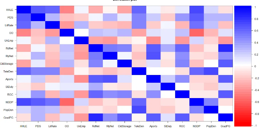
Initially 20 variables were identified and their correlations evaluated. For variables with high correlation valuesamongst them, the author felt the need for testing of multi collinearity; a situation in which two or more explanatory variables is highly related linearly and contain almost the same information about the dependent variable. Multicollinearity was tested using VIF (variance inflation factor). Variables having VIF> 10 were identified and dropped from the study. After dropping 5 such variables, Corplot was extracted once again [Fig 1] and VIF outputsuggested absence of multicollinearity sinceits valuesfor all the 15 retained variables were found to be< 10 (Fig 2).

vif(data)

Fig 2: VIF Table; Source - R output from Secondary Data

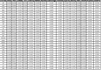
Fig 3 below presents the performance table. The actual data of the 15 variables (criterions) for all the alternatives is captured in the form of a matrix known as decision matrix or performance matrix / table. It is to be noted that many criterions have varying or different units and before making any further multi criteria decision making analysis, the effect of such disparate units need to be eliminated and the same was done by performing statistical normalization. The normalized performance table is shown in Fig 4.Subsequent calculations (Shannon‟s weight, group utility, individual regret and VIKOR index)were done with normalized data.

[Notations used in study - HHLE: % of households having electricity, PDS: % of households having pucca dwelling structure, LitRate: Overall State literacy rate, OO: Households having Owned Occupancy (in „000), UnEmp: Unemployment rate (per „000), RdNet: Road Network (in km), RlyNet: Railway Network (in km), CldStorage: Cold Storage capacity (MT), TeleDen: Telecommunication density, Aports: No. of Air ports in the state, StDuty: Stamp duty in the state (in %), RGC: Rural Godown Capacity, NSDP: Per capita Net State Domestic Product, PopDen: Population Density, GradPG: No. of Graduates & Post Graduates]

HHLE PDS LitRate OO UnEmp RdNet RlyNet CldStorage 7.21 4.40 2.77 1.94 1.81 8.15 3.65 6.01

Performance & Normalized Performance Tables

Fig 3: Performance Table; Source - Secondary Data

Fig 4: Normalized Performance Table; Source–R Output from Secondary Data

STATES HHLE PDS LitRate OO UnEmp RdNet RlyNet CldStorage TeleDen Aports StDuty RGC NSDP PopDen GradPG

AP 92.2 77.1 67.02 78.47 39 179022 3703.25 1782561 89.03 5 5 69.264 72301 303 2796965

ARP 65.7 33.9 65.38 68.32 89 25362 11.67 6000 85.6 1 6 0.22 76370 17 44466

ASM 37 27 72.19 87.92 61 326512 2442.57 157906 62.38 3 6 15.85 38945 397 500787

BIH 16.4 48.3 61.8 96.79 60 206010 3730.57 1415595 56.91 3 6 17.16 26948 1102 1309800

CHA 75.3 39.4 70.28 90.2 19 97534 1212.91 484087 62.49 1 7.5 35.54 53815 189 397779

DEL 99.1 94.7 86.21 68.21 36 32067 183.23 129857 236.38 1 5 4.49 185421 11297 701156

GOA 96.9 86 88.7 78.95 96 14624 69.31 7705 101.7 1 7 0.37 200514 394 61640

GUJ 90.4 75.7 78.03 83.92 9 182287 5258.49 2901807 104.05 7 3.5 47.84 93046 308 1415546

HAR 90.5 94.8 75.55 88.36 47 46287 1710.49 749830 84.08 1 5 99.5 119833 573 757974

HP 96.8 80.6 82.8 87.2 106 55593 296.26 131017 185.42 3 8 2.57 83899 123 202217

J & K 85.1 68.3 67.16 96.72 72 39096 298.19 112516 84.47 3 5 1.61 52386 57 264350

JH 45.8 43 66.41 89.28 77 42705 2394.46 236680 56.91 4 6 2.09 40238 414 327729

KAR 90.6 63.5 75.36 74.25 15 321808 3281.36 560178 106.29 5 7 60.37 77168 319 1783902

KER 94.4 80.3 94 90.68 125 194854 1045.36 80405 107.81 3 7 12.86 91567 859 706353

MP 67.1 56.9 69.32 90.87 43 288931 5000 1263665 62.49 6 8 121.89 43426 236 1166426

MAHA 83.9 78.9 82.34 81.12 21 608140 5745.48 978392 101.7 6 7 102.57 103856 365 3564610

MAN 68.3 17 79.21 93.69 57 24247 1.35 5500 85.6 1 6 0.54 37656 122 123456

MEGH 60.9 51.4 74.43 81.97 48 13372 8.76 8200 85.6 1 6 0.86 54156 132 64226

MIZ 84.2 67.1 91.33 66.06 30 9831 1.5 4001 85.6 1 6 0.39 63413 52 29846

NAG 81.6 55.2 79.55 73.75 85 37176 11.13 7350 85.6 1 6 0.5 70274 119 56346

ORI 43 40.3 72.87 90.34 50 283692 2572.16 540141 74.83 3 7 24.42 49227 269 768591

PUN 96.6 93.4 75.84 88.87 60 105368 2269.27 2155704 114.28 3 5 138.62 84512 550 628638

RAJ 67 73.8 66.11 93.22 71 248156 5893.1 555278 86.11 4 8 47.69 60844 201 1499267

SIK 92.5 62.5 81.42 64.84 181 7450 1 2100 84.72 1 6 0.1 151395 86 18815

TN 93.4 73.5 80.09 74.55 42 261100 4027.08 337625 120.6 8 8 38.98 98628 555 2384481

TRI 68.4 19.2 87.22 91.81 197 37384 192.54 45477 85.6 1 6 1.02 57402 350 63850

UP 36.8 67.8 67.68 94.7 74 415383 339.8 14176062 68.2 2 6 104.63 33482 828 3883292

UT 87 93.9 79.63 82.87 70 62945 9077.45 160419 68.2 2 4 28.56 92566 189 337806

WB 54.5 50.3 76.26 89.28 49 295997 4135.19 5947561 84.72 4 6 32.6 60318 1029 1318457

STATES HHLE PDS LitRate OO UnEmp RdNet RlyNet CldStorage TeleDen Aports StDuty RGC NSDP PopDen GradPG

AP 0.2206 0.2158 0.1621 0.1723 0.0916 0.1559 0.2125 0.1107 0.1644 0.2617 0.1479 0.2383 0.1514 0.0262 0.3709 ARP 0.1572 0.0949 0.1581 0.1500 0.2090 0.0221 0.0007 0.0004 0.1581 0.0523 0.1775 0.0008 0.1599 0.0015 0.0059 ASM 0.0885 0.0756 0.1746 0.1931 0.1432 0.2844 0.1401 0.0098 0.1152 0.1570 0.1775 0.0545 0.0815 0.0343 0.0664 BIH 0.0392 0.1352 0.1494 0.2126 0.1409 0.1794 0.2140 0.0879 0.1051 0.1570 0.1775 0.0590 0.0564 0.0953 0.1737 CHA 0.1801 0.1103 0.1699 0.1981 0.0446 0.0849 0.0696 0.0301 0.1154 0.0523 0.2219 0.1223 0.1127 0.0164 0.0527 DEL 0.2371 0.2651 0.2085 0.1498 0.0845 0.0279 0.0105 0.0081 0.4365 0.0523 0.1479 0.0155 0.3883 0.9774 0.0930 GOA 0.2318 0.2407 0.2145 0.1734 0.2254 0.0127 0.0040 0.0005 0.1878 0.0523 0.2071 0.0013 0.4199 0.0341 0.0082 GUJ 0.2163 0.2119 0.1887 0.1843 0.0211 0.1588 0.3017 0.1803 0.1921 0.3664 0.1035 0.1646 0.1948 0.0266 0.1877 HAR 0.2165 0.2653 0.1827 0.1940 0.1104 0.0403 0.0981 0.0466 0.1553 0.0523 0.1479 0.3424 0.2509 0.0496 0.1005 HP 0.2316 0.2256 0.2002 0.1915 0.2489 0.0484 0.0170 0.0081 0.3424 0.1570 0.2367 0.0088 0.1757 0.0106 0.0268

J & K 0.2036 0.1912 0.1624 0.2124 0.1691 0.0341 0.0171 0.0070 0.1560 0.1570 0.1479 0.0055 0.1097 0.0049 0.0351

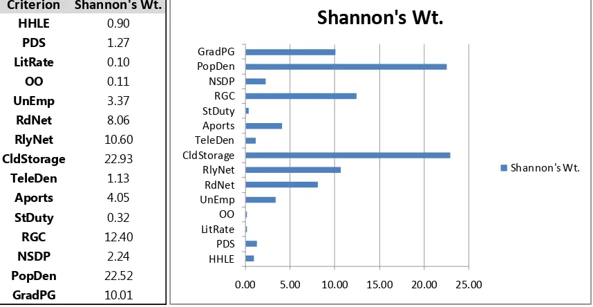
Fig 5: Shannon‟s Weight Table; Source - R output from Secondary Data

Shannon‟s weights also known as entropy weight have been evaluated for 15 variables

included in the study and the same is shown in Fig 5. These weights indicate the relative importance of the parameters in a multi criteria environment influencing retailing. The weights vary from as low as 0.1% to 22.93%. Cold storage capacity and population density are the two most important parameters accounting for more than 45% of the overall criteria importance. Logistics support in the form of road and railway network contribute to almost 19% while rural godown/ warehousing capacity and educated portion of the population have relative importance levels at 12.4% and 10% respectively. These 6 variables account for about 86% of the total importance.

Fig 6:VIKOR Output; Source - R output from Secondary Data

Criterion Shannon's Wt.

HHLE 0.90 PDS 1.27 LitRate 0.10 OO 0.11 UnEmp 3.37 RdNet 8.06 RlyNet 10.60 CldStorage 22.93 TeleDen 1.13 Aports 4.05 StDuty 0.32 RGC 12.40 NSDP 2.24 PopDen 22.52 GradPG 10.01 HHLE PDS LitRate OO UnEmp RdNet RlyNet CldStorage TeleDen Aports StDuty RGC NSDP PopDen GradPG

0.00 5.00 10.00 15.00 20.00 25.00

Shannon's Wt.

Shannon's Wt.

STATES S R Q Rank STATES S R Q Rank

AP 0.4519 0.2005 0.6561 6 MAHA 0.3703 0.2135 0.6233 3

ARP 0.6284 0.2292 0.8734 24 MAN 0.6286 0.2292 0.8736 25

ASM 0.5887 0.2268 0.8348 16 MEGH 0.6235 0.2292 0.8694 22

BIH 0.5920 0.2064 0.7852 11 MIZ 0.6142 0.2293 0.8620 20

CHA 0.5777 0.2215 0.8123 14 NAG 0.6225 0.2292 0.8685 21

DEL 0.7840 0.2272 0.9947 29 ORI 0.5663 0.2206 0.8008 13

GOA 0.6094 0.2292 0.8579 19 PUN 0.4464 0.1945 0.6362 4

GUJ 0.4849 0.1824 0.6364 5 RAJ 0.5571 0.2204 0.7926 12

HAR 0.5098 0.2172 0.7461 9 SIK 0.6318 0.2293 0.8763 26

HP 0.5950 0.2272 0.8411 17 TN 0.4910 0.2239 0.7480 10

J & K 0.6011 0.2275 0.8468 18 TRI 0.6560 0.2286 0.8942 27

JH 0.6359 0.2255 0.8699 23 UP 0.1687 0.0347 0.0000 1

KAR 0.4798 0.2203 0.7296 8 UT 0.6725 0.2267 0.9028 28

KER 0.5847 0.2280 0.8348 15 WB 0.4774 0.1331 0.5037 2

MP 0.4625 0.2089 0.6863 7

Fig 7: VIKOR Scatter Plot Matrix(S, R & Q);Source - R output from Secondary Data

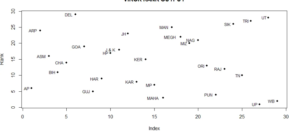
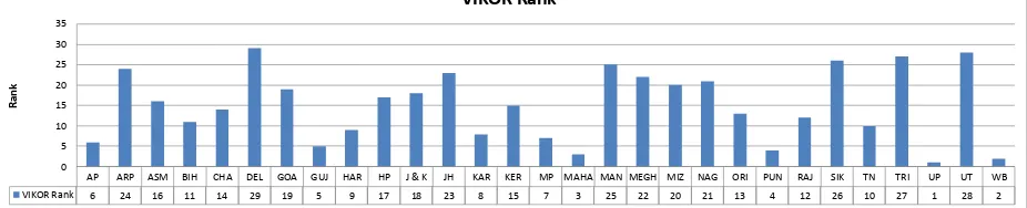
Fig 8B: VIKOR Output (State Ranks); Source - R output from Secondary Data

F.

Conclusion

The study reveals Uttar Pradesh as the best alternative i.e. state with highest retailing potential in India and the remaining states in the list of top ten includes West Bengal, Maharashtra, Punjab, Gujarat, Andhra Pradesh, Madhya Pradesh, Karnataka, Haryana and Tamil Nadu in order of decreasing retailing potential. Cold storage, population density, rural godown capacity, education status, road and railway network have emerged as factors influencing retailing potential in order of decreasing importance.

G.

Limitations & Scope of Further Study

Subjective parameters that may influence retailing, like political stability and organization‟s perception on industrial climate in a state, have not been considered. One may use other ranking methods to analyze the same in future and comparison made thereof.

H.

Bibliograpy

 (2005). India’s Retailing Potential, Association of Indian Individual Investors.  (2005). Retail Growth in India, KPMG.

 (2007). Organized Retail Expansion in India, New Delhi: Ministry of Commerce &

Industry, Government of India.  (2008). Annual Report, NCAER

 (2008). RK Swamy Guide to Market Planning

 (2013). All India Survey On Higher Education 2010-11. Department Of Higher

Education. New Delhi: Ministry Of Human Resource Development.

 (2013). State Of Housing In India a Statistical Compendium. Ministry of Housing and

Urban Poverty Alleviation National Buildings Organisation, Government of India. AP ARP ASM BIH CHA DEL GOA GUJ HAR HP J & K JH KAR KER MP MAHA MAN MEGH MIZ NAG ORI PUN RAJ SIK TN TRI UP UT WB VIKOR Rank 6 24 16 11 14 29 19 5 9 17 18 23 8 15 7 3 25 22 20 21 13 4 12 26 10 27 1 28 2

0 5 10 15 20 25 30 35

R

an

k

 (2013-14 & 2014-15). Basic Road Statistics Of India. New Delhi: Ministry Of Road

Transport Aand Highways Transport Research Wing.

 (2014). Retail Realty in India: Evolution and Potential. A Comparison and Contrast

with the Emerging Cities of Asia. Retail Intelligence.

 (2015-16). Augmenting Rural Storage Infrastructure Through Scheme Of Rural

Godowns. Department Of Agriculture, Cooperation And Farmers Welfare. New Delhi: Ministry Of Agriculture And Farmers Welfare.

 (2015-16). Fifth Annual Employment - Unemployment Survey. Chandigarh: Ministry

Of Labour & Employment Labour Bureau.

 (2016). Highlights of Telecom Subscription Data. New Delhi: Telecom Regulatory

Authority of India.

 (2016). Retail. Indian Brand Equity Foundation.

 (2017). Indian Retail Industry - Structure & Prospects. Mumbai: CARE Ratings

Professional Risk Opinion.

 (2017). Retail. Indian Brand Equity Foundation.

 Agarwal, P. (2012). Potential Of Organized Retail In India. International Journal of Engineering And Management Science, 3 (4), 456-460.

 Cencus of India 2011. (2011). Retrieved 2017, from http://www.censusindia.gov.in:

http://www.censusindia.gov.in/2011census

 Dashore, K., Singh Pawar, S., Sohani, N., & Singh Verma, D. (2013). Product

Evaluation Using Entropy and Multi Criteria Decision Making Methods. International Journal of Engineering Trends and Technology, 4 (5), 2183-2187.  Executive summary of month of November 2015. (2015). Retrieved from Central

Electricity Authority: http://www.cea.nic.in/

 Kahraman, C., Ruan, D., &Dogan, I. (2003). Fuzzy group decision-making for

facility location selection. information sciences, 135-153.

 Kargi, V. S. (2016). Supplier Selection for A Textile Company Using The Fuzzy

TOPSIS Method. Manisa Celal Bayar Üniversitesi İ.İ.B.F., 23 (3), 1-15.

 List of airports in India. (2016, November). Retrieved 2017, from Wikipedia:

https://en.wikipedia.org/wiki/List_of_airports_in_India

 Onut, S., &Soner, S. (2008). Transshipment site selection using the AHP and TOPSIS

 Per Capita NSDP at current prices (2004-05 to 2014-15). (2015). Retrieved from

NITI Aayog: http://niti.gov.in/content/capita-nsdp-current-prices-2004-05-2014-15  Rani, S. (2013). Retail Industry In India (A Study On Growth Development

Opportunities And Challenges). International Journal of Computing and Corporate Research, 3 (6).

 Shannon, C (1948). A Mathematical Theory of Communication, Bell System

Technical Journal, 27 (July and October), pp. 379–423, 623–656.

 Singh, P. K. (2014). Retail Sector in India: Present Scenario, Emerging Opportunities

and Challenges. IOSR Journal of Business and Management, 16 (4), 72-81.

 Stamp Duty Caluclator for Property registration. (2017). Retrieved from

TodayPriceRates:http://property.todaypricerates.com/stamp-duty-registration-percentage-value-calculator

 State wise distribution of Cold Storage capacity. (2017, July). Retrieved from Press

Information Bureau: http://pib.nic.in/newsite/PrintRelease.aspx?relid=168990



 Venkatesh, N. (2013). Indian Retail Industries Market Analysis: Issues, Challenges