for Optimal Sensing
Philipp del Hougne,1,∗ Mohammadreza F. Imani,2 Aaron V. Diebold,2Roarke Horstmeyer,3and David R. Smith2 1Institut de Physique de Nice, CNRS UMR 7010, Universit´e Cˆote d’Azur, Nice, France
2Department of Electrical and Computer Engineering,
Duke University, Durham, North Carolina, USA
3
Biomedical Engineering Department, Duke University, Durham, North Carolina, USA
(Dated: June 26, 2019)
We address the fundamental question of how to optimally probe a scene with electromagnetic (EM) radiation to yield a maximum amount of information relevant to a particular task. Machine learning (ML) techniques have emerged as powerful tools to extract task-relevant information from a wide variety of EM measurements, ranging from optics to the microwave domain. However, given the ability to actively illuminate a particular scene with a programmable EM wavefront, it is often not clear what wavefronts optimally encode information for the task at hand (e.g., object detection, classification). Here, we show that by integrating a physical model of scene illumination and detection into a ML pipeline, we can jointly learn optimal sampling and measurement processing strategies for a given task. We consider in simulation the example of classifying objects using microwave radiation produced by dynamic metasurfaces. By integrating an analytical forward model describing the metamaterial elements as coupled dipoles into the ML pipeline, we jointly train analog model weights with digital neural network weights. The learned non-intuitive illumination settings yield a higher classification accuracy using fewer measurements. On the practical level, these results are highly relevant to emerging context-aware systems such as autonomous vehicles, touchless human-interactive devices or within smart health care, where strict time constraints place severe limits on measurement strategies. On the conceptual level, our work serves as a bridge between wavefront shaping and tunable metasurface design on the physical layer and ML techniques on the processing layer.
I. INTRODUCTION
Wave-based sensing is of fundamental importance in countless applications, ranging from medical imaging to non-destructive testing [1]. Currently, it is emerging as key enabling technology for futuristic “context-aware” concepts like autonomous vehicles [2, 3], ambient-assisted living facilities [4, 5] and touchless human-computer in-teraction (HCI) devices [6, 7]. In these context-aware settings, an important goal is often to achieve the high-est possible accuracy for a given task, such as recogniz-ing a hand gesture, with as few measurements as possi-ble. Minimizing the number of measurements can help improve a wide number of metrics - for example, speed, power consumption, and device complexity. It is also cru-cial in a variety of specific contexts - for instance, to limit radiation exposure (e.g., x-ray imaging [8]), to adhere to strict timing constraints caused by radiation coherence or unknown movements in a biological context [9–11], or to make real-time decisions in automotive security [3, 12].
In all of the above applications, “active” illumination is sent out from the device to interact with the scene of interest before the reflected waves are captured by the sensor. The resulting measurements are then pro-cessed to achieve a particular goal. Usually, acquisition and processing are treated and optimized separately. For instance, the spatial resolution of a LIDAR system on
an autonomous vehicle is often optimized to be as high as possible, while its resulting measurements are subse-quently processed to detect pedestrians with as high an accuracy as possible. Recently, machine learning (ML) techniques have dramatically improved the accuracy of measurements post-processing for complex tasks (like ob-ject recognition) without requiring explicit analytical in-structions [13–18].
However, to date, the physical acquisition layers of context-aware systems have yet to reap the benefits of new ML techniques. At the same time, by separately op-timizing acquisition hardware and post-processing soft-ware, most sensing setups are not tailored to their specific sensing task. Instead, as with the LIDAR example noted above, hardware is typically optimized to obtain a high-fidelity visual image for human consumption, thereby of-ten ignoring available knowledge that could help to high-light information that is critical for ML-based analysis.
Here, we address both of the above shortcomings with a new “learned sensing” paradigm for context-aware sys-tems that allows for joint optimization of acquisition hardware and post-processing software. The result is a device that acquires non-imaging data that is optimized for a particular ML task. We consider the challenge of identifying settings of a reconfigurable metamaterial-based device emitting microwave patterns that can en-code as much relevant information about a scene for subsequent ML-based classification with as few measure-ments as possible. However, as we will detail, this frame-work is general, flexible, and can impact a number of
2
future measurement scenarios.
II. ILLUMINATION STRATEGIES IN WAVE-BASED SENSING
A number of prior works have attempted to optimize active illumination in the microwave, terahertz, and opti-cal regimes to improve the performance of certain sensing tasks. The simplest approach in terms of the transceiver hardware is often to use random illumination, for in-stance, by leveraging the natural mode diversity available in wave-chaotic or multiply-scattering systems [19–22]. Random illuminations have a finite overlap that reduces the amount of information that can be extracted per ad-ditional measurement. A truly orthogonal illumination basis, such as the Hadamard basis [23–26], has also been frequently used to overcome this (minor) issue, often at the cost of more complicated hardware.
These forms of “generic” illumination often fail to ef-ficiently highlight salient features for task-specific sens-ing, which is desirable to reduce the number of required measurements. In other words, they do not discriminate between relevant and irrelevant information for the task at hand. Task-specific optimal illumination can be chal-lenging to determine, due to hardware constraints (e.g., few-bit wavefront modulation), possible coupling effects between different transceivers, and in particular a lack of insight into the inner workings of the ML network (i.e., the artificial neural network, ANN) used to process the acquired data for each task. So far, most attempts at task-specific tailored illuminations seek to synthesize il-lumination wavefronts matching the expected principal components of a scene [27–30]. To outperform generic il-lumination, such an approach requires a sufficiently large aperture with a sufficient amount of tunable elements to synthesize wavefronts in reasonable agreement with the expected principal components. Moreover, a sufficient number of measurements has to be taken to cover the most important principal scene components.
Approaches based on a principal component analysis (PCA) of the scene can thus be interpreted as a step towards optimal wave-based sensing (see Fig. S3 in the Supplemental Material); they work well under favorable conditions (large aperture, many tunable elements, un-restricted number of measurements). However, the fun-damental challenge of extracting as much task-relevant information as possible using a general wave-based sen-sor thus remains open. Besides its fundamental interest, the question is also of high relevance to many practical applications: for instance, in automotive RADAR and LIDAR, the aperture size, the number of tunable illu-mination elements, and the measurement sampling rate over space and time are all highly restricted. In these constrained scenarios, we hypothesize that wave-based sensing can benefit from joint optimization of data ac-quisition and processing.
Inspired by recent works in the optical domain [12, 32],
this work interprets data acquisition as a trainable physi-cal layer that we integrate directly into an ANN pipeline. By training the ANN with a standard supervised learn-ing procedure, we can simultaneously determine opti-mal illumination settings to encode relevant scene in-formation, along with a matched post-processing algo-rithm to extract this information from each measurement — automatically taking into account any constraints on transceiver tuning, coupling and the number of allowed measurements.
As noted above, we apply our concept to classification tasks with microwave sensors. These tasks are a crucial stepping stone towards numerous context-aware systems e.g. in smart homes, for hand gesture recognition with HCI devices, for concealed-threat identification in secu-rity screening, and in autonomous vehicles [2–7]. Mi-crowave frequencies can operate through optically opaque materials such as clothing, are not impacted by external visible lighting and scene color, minimally infringe upon privacy (unlike visual cameras) and may eventually help sense through fog, smoke and “around-the-corner” [7].
We focus on optimally configuring dynamic metasur-face hardware, a promising alternative to more tradi-tional antenna arrays for beam-forming and wavefront shaping [23]. Dynamic metasurfaces are electrically large structures patterned with metamaterial elements that couple the modes of an attached waveguide or cavity to the far field [24, 25]. Reconfigurability is achieved by indi-vidually shifting each metamaterial element’s resonance frequency, for instance, with a PIN diode [5]. Compared to a traditional antenna array that uses amplifiers and phase shifters, the inherent analog multiplexing makes dynamic metasurface hardware much simpler, less costly and easier to integrate in many applications.
To demonstrate our proposed Learned Integrated Sens-ing Pipeline (LISP), we jointly optimize the illumina-tion and detecillumina-tion properties of dynamic metasurface transceivers, along with a simple neural network classi-fier, for the task of scene classification. In this work, we consider the dummy task of classifying “handwritten” metallic digits in simulation. Replacing this dummy task with a more realistic scenario, such as concealed-threat detection, hand-gesture recognition or fall detection, is conceptually straight-forward. To construct the LISP, we first formulate an analytical forward model which is possible due to the intrinsic sub-wavelength nature of the metamaterial elements. Second, we allow certain key pa-rameters within the “physical” forward model to act as unknown weights (here the reconfigurable resonance fre-quency of each metamaterial element), that we aim to optimize over. Third, we then merge this weighted phys-ical model into an ANN classifier, and use supervised learning to jointly train the unknown weights in both to maximize the system’s classification accuracy. Despite coupling between metamaterial elements and a binary tuning constraint, which would otherwise be challenging to account for in a standard inverse model, our ANN im-plicitly accounts for this during training and identifies
si-multaneously optimal illumination settings and process-ing structures to extract as much task-relevant informa-tion as possible. We are also easily able to use this model to compare the performance of our scheme with the afor-mentioned benchmarks of orthogonal and PCA-based il-lumination.
Interestingly, our LISP can also be interpreted in light of recent efforts to meet the exploding computational demands of ANNs with wave-based analog computing, which seeks to perform desired operations with waves as they interact with carefully tailored systems [36–43]. Our wave-based sensing scheme is essentially a hybrid analog-digital ANN in which the interaction of learned optimal wavefronts with the scene acts as a first processing layer. As we will show, data acquisition fulfills two processing tasks in our pipeline, being (i) trainable and (ii) highly compressive.
III. OPERATION PRINCIPLE
This section is outlined as follows: first, we introduce the hardware of our reconfigurable metasurface aper-tures. Second, we establish an analytical forward model of our sensor’s physical layer built upon a compact de-scription of the metamaterial elements as dipoles. It consists of three steps: (i) extracting each metamaterial element’s dipole moment while taking tuning state and inter-element coupling into account; (ii) propagating the radiated field to the scene; (iii) evaluating the scattered field. Third, we outline the sensing protocol. Finally, fourth, we integrate analog (physical) and digital (pro-cessing) layers into a unique ANN pipeline and discuss how it can be trained and account for binary reconfig-urability constraints.
Note that this section seeks to give a clear and thor-ough overview of the physical layer and its integration into the ANN pipeline by only providing key equations; details, derivations and equations defining all variables are included in Section A of the Supplemental Material for completeness, following Refs. [1, 2].
A. Dynamic Metasurface Aperture
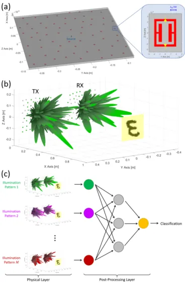
The reconfigurable metasurface that we consider for the generation of shaped wavefronts is depicted in Fig. 1(a). It consists of a planar metallic waveguide that is excited by a line source (a coaxial connector in a practical implementation). N metamaterial elements are patterned into one of the waveguide surfaces to couple the energy to free space. An example of a metamaterial element that could be used is the tunable complimen-tary electric-LC (cELC) element [5] shown in the inset of Fig. 1(a). A possible tuning mechanism to individually configure each metamaterial element’s radiation proper-ties involves diodes. Then, the cELC element is resonant or not (equivalently, radiating or not radiating) at the
FIG. 1. Schematic overview of operation principle. (a) Dy-namic metasurface. N = 64 tunable metamaterial ele-ments are patterned into the upper surface of a planar waveg-uide. The inset shows the geometry of an example cELC metamaterial element that could be used in combination with PIN diodes (location and orientation indicated in yellow) to reconfigure the element. The waveguide is excited by the in-dicated line source. (b)Sensing setup. The scene consists of a metallic digit in free space that is illuminated by a TX metasurface and the reflected waves are captured by a second RX metasurface. (c)Sensing protocol. The scene is illu-minated withM distinct TX-RX metasurface configurations, yielding a 1×M complex-valued measurement vector that is processed by an artificial neural network consisting of fully connected layers. The output is a classification of the scene.
working frequency off0= 10 GHz depending on the bias voltage of two PIN diodes connected across its capacitive gaps. The N metamaterial elements are randomly dis-tributed within a chosen aperture size (30 cm×30 cm) but a minimum distance between elements of one free-space wavelength is imposed [6].
Similar dynamic metasurfaces have previously been used to generate random scene illuminations for
com-4
putational imaging [24, 25]. Here, we will take full ad-vantage of the ability to individually control each radi-ating element to purposefully shape the scene illumina-tions. The individual addressablility of each metama-terial element distinguishes these dynamic metasurfaces from other designs in the literature that simultaneously reconfigure all elements to redirect a beam [47–49]. Our LISP could of course also be implemented with other wavefront shaping setups such as arrays of reconfigurable antennas [23], reflect-arrays illuminated by a separate feed (e.g. a horn antenna) [50–52] or leaky-wave antennas with individually controllable radiating elements [53, 54]. Indeed, if our concept was transposed to the acoustic or optical regime, one would probably use an array of acous-tic transceivers or a spatial light modulator, respectively. In the microwave domain, however, antenna arrays are costly and the use of reflect-arrays yields bulky setups. In contrast, dynamic metasurface hardware as the one in Fig. 1(a) benefits from its inherent analog multiplex-ing and is moreover compact, planar and can be fabri-cated using standard PCB processes. Note that although we focus for concreteness on an implementation that we consider advantageous, our ideas are not limited to this specific hardware.
B. Compact Analytical Forward Model
The formulation of a compact analytical forward model is enabled by the intrinsic sub-wavelength nature of the radiating metamaterial elements which enables a conve-nient description in terms of (coupled) dipole moments [55–58]. Ultimately, we will directly link a given meta-surface configuration (specifying which elements are ra-diating) to the radiated field. Note that the possibility to analytically do so is a key advantage of this metasurface hardware over alternative devices with reconfigurable ra-diation pattern such as leaky reconfigurable wave-chaotic three-dimensional cavities [59–61]. For the latter, one could learn forward models based on near-field scans of radiated fields [22, 23]; yet the number of required equiva-lent source dipoles [2] (even with a coarse half-wavelength sampling of the aperture) is much higher than in our case where it is simplyN.
1. Dipole Moments
Generally speaking, a point-like scatterer’s magnetic dipole momentmis related to the incident magnetic field
Hloc via the scatterer’s polarizability tensorα:
m(r) =αHloc(r), (1)
where r denotes the scatterer’s location. In our case, using surface equivalent principles, an effective polariz-ability tensor of the metamaterial element embedded in
the waveguide structure can be extracted [3]. For the metamaterial element we consider, only the αyy com-ponent is significant. In the following, we use αyy = (1.5−3.5i)×10−7 m3 which is a typical polarizability value for a tunable cELC element [3] [9]. The tuning state of a given metamaterial element can be encoded in its polarizability: if the element is “off”, its polariz-ability (at the working frequency) is zero and hence it does not radiate any energy. We thus usetj,iαyy as effec-tive polarizability, wheretj,i∈ {0,1} is the tuning state of thejth metamaterial element in the ith metasurface configuration.
The local magnetic field Hloc that excites the meta-material element is a superposition of the feed wave and the fields scattered off the other metamaterial elements.
Hloc in Eq. S1 is thus itself a function of the metama-terial elements’ magnetic dipole moments, yielding the following system of coupled equations [1]:
Hyloc(rj) = (tj,iαyy)−1 my(rj), (2a)
Hyloc(rj) =Hyf eed(rj) +
X
j6=k
Gyy(rj,rk)my(rk), (2b)
where Eq. 2a is a rearranged version of Eq. S1 and the in-dexiidentifies theith metasurface configuration. Equa-tion 2b expresses the local field at locaEqua-tionrj as sum of the feed waveHf eed
y at rj and the individual contribu-tions from each of the other metamaterial elements at
rk 6= rj via the Green’s functions Gyy(rj,rk). Explicit expressions forHf eed
y (rj) andGyy(rj,rk) are provided in the Supplemental Material. To solve Eq. S6 for the mag-netic dipole moments we rewrite it in matrix form and perform a matrix inversion, as shown in Step 1A in the top line of Fig. 2:
Mi={Ai−G}−1F, (3)
where Mi = [my,i(r1), my,i(r2), . . . , my,i(rN)], Ai = diag
t1,iαyy)−1,(t2,iαyy)−1, . . . ,(tN,iαyy)−1
andF=
Hyf eed(r1), Hyf eed(r2), . . . , Hyf eed(rN)
. The off-diagonal entry (j, k) ofGisGyy(rj,rk), and the diagonal ofGis zero since the self-interaction terms are incorporated into the effective polarizabilities inAi[66].
Due to the metamaterial element interactions via the Gyy(rj,rk) term, the mapping from tuning state to dipole moments is not linear. This is visualised with an ex-ample in Fig. S1. Thus, ultimately the mapping from tuning state to radiated field cannot be linear, which is a substantial complication for most beam synthesis ap-proaches; as we will see in Section III D, this does not pose any additional complication in our LISP.
2. Propagation to Scene
Having found a description of the metamaterial ele-ments in terms of dipole moele-ments, we can now go on
to identify the wavefront impacting the scene for a given metasurface configuration. The sensing setup we con-sider is depicted in Fig. 1(b). A transmit (TX) metasur-face like the one discussed above illuminates the scene. The scene, in our case, consists of a planar metallic digit of size 40 cm×40 cm in free space that is to be recognized at a distance of 1 m.
To compute the ith incident TX wavefront (corre-sponding to the ith metasurface configuration) at a lo-cationζin the scene, we superimpose the fields radiated by each of theN metamaterial element dipoles [2, 29]:
ETXi (ζ) = −iωµ0 4π N X j=1 (mi(rj)×ρˆj) −ik Γj − 1 Γ2 j ! e−ikΓj ! , (4) whereω = 2πf0, Γj =|ζ−rj|, ˆρj is a unit vector paral-lel to ζ−rj andmi(rj) is the magnetic dipole moment of the jth metamaterial element in the ith metasurface configuration. Equation S13 is the second step of our analytical forward model, as shown in Step 1B in Fig. 2. Since the magnetic dipole moments only have a signifi-canty-component, the radiated electric field’s dominant component is alongz.
3. Measurement
To complete the physical layer description, we need to identify the portion of TX fields that is reflected off the scene and collected by the second receiving (RX) meta-surface, as shown in Fig. 1(b). Since our scene is flat and reflections are primarily specular, the first Born ap-proximation is a suitable description: the field reflected at locationζin the scene isETX
i (ζ)σ(ζ), whereσis the scene reflectivity. The RX metasurface captures specific wave forms depending on its configuration; their shape is essentially defined via a time-reversed version of Eq. S13. The complex-valued signal measured for the ith pair of TX-RX configurations is thus [2]
gi∝
Z
scene
ETXi (ζ)·ERXi (ζ)σ(ζ) dζ. (5)
This is the third and final step of our analytical forward model, shown as Step 1C in Fig. 2. Note that the scene σ(ζ) is ultimately sampled byIi(ζ) =ETXi (ζ)·ERXi (ζ); when loosely referring to “scene illumination” in this work, we mean this product ofETX
i (ζ) andERXi (ζ). [68] In practice, to compute the integral, we discretize the scene at the Rayleigh limit, that is the scene consists of a 28×28 grid of points with half-wavelength spac-ing. Each point’s reflectivity value σ(ζ) is a gray-scale real value determined by the corresponding handwritten digit’s reflectivity map.
C. Sensing Protocol
Having outlined the physical layer of our sensing setup, we next consider the sensing protocol. A single measure-ment, depending on various factors such as the sensing task’s complexity, the type of scene illumination but also the signal-to-noise ratio, may not carry enough informa-tion to successfully complete the desired sensing task [69]. Hence, in general, we illuminate the scene with M dis-tinct patterns. Each pattern corresponds to a specific pair of TX and RX metasurface configurations. Since our scheme is monochromatic, each measurement yields a single complex valuegi.
As shown in Fig. 1(c), our 1×M complex-valued mea-surement vector is fed into a processing ANN. The latter consists of two fully connected layers. Real and imagi-nary parts of the measurement vector are stacked and the resultant real-valued vector is the input to the first layer consisting of 256 neurons with ReLu activation. This is followed by a second fully connected layer made up of 10 neurons with SoftMax activation, yielding a nor-malized probability distribution as output. (See Supple-mental Material for details.) The highest value therein corresponds to the classification result (one digit between “0” and “9”). These are the two digital layers shown in Fig. 2. This architecture was chosen without much op-timization and still performs quite well; its performance was observed to not significantly depend on the chosen parameters, such as the number of neurons.
D. Hybrid Analog-Digital ANN Pipeline
We are now in a position to assemble our pipeline consisting of an analog and two digital layers as out-lined above (Fig. 2). The input, a scene, is injected into the analog layer which contains trainable weights and is moreover highly compressive. The output from the analog layer, the measurement vector, continues to be processed by the digital layers which contain train-able weights as well. The final digital layer’s output is the classification of the scene. By jointly training the analog and the digital weights, we identify illumination settings that optimally match the constraints and pro-cessing layer. Importantly, this means that the ANN will find an optimal compromise also in cases where the aper-ture size is small and few tunable elements are available, meaning that PCA modes cannot be synthesized accu-rately, and when the number of measurements is very limited, meaning that not all significant PCA modes can be probed.
While the digital weights (b(1)p , w (1) p,i, b (2) c and w (2) c,p in Fig. 2) are real-valued variables drawn from a continu-ous distribution, our metasurface hardware requires the physical weights tj,i to be binary. At first sight, this constraint is incompatible with variable training by back-propagating errors through the ANN which relies on com-puting gradients [11]. An elegant solution consists in
6
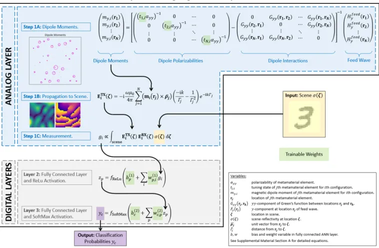
FIG. 2. Overview of our Learned Integrated Sensing Pipeline (LISP). The analog (physical) layer corresponds to the sensing setup introduced in Fig. 1(b). A scene is illuminated with a dynamic metasurface, and the reflected waves are captured with a second metasurface. The analytical forward model for the analog layer consists of three steps. First, each metamaterial element’s magnetic dipole moment is calculated for a given metasurface configuration. The inset shows an example of calculated dipole moments which are represented as phasors, with the radius of the circle being proportional to their amplitude, and the line segment showing their phase. The circles are centered on the physical location of each metamaterial element. Second, the field radiated by these dipoles to the scene is computed. The inset shows amplitude (left) and phase (right) of a sample field illuminating the scene. Third, the measurement is evaluated. Note that the figure contains the equations for Steps 1A and 1B only for the TX metasurface, for the sake of clarity; the RX equations are analogous. The measurement vector, consisting of complex-valued entries corresponding to different configurations of the TX-RX metasurfaces, is then processed by two fully connected layers consisting of 256 and 10 neurons, respectively. Finally, a classification of the scene is obtained as output. Trainable weights in our hybrid analog-digital ANN pipeline are both in the analog and the digital layers and highlighted in green. During training, these are jointly optimized via error back-propagation.
the use of a temperature parameter that supervises the training, gradually driving the physical weights from a continuous to a discrete binary distribution [12]. The de-tailed implementation thereof is outlined in Section B.2 of the Supplemental Material. Note that we ultimately only have to formulate an analytical forward model; the fact that this model contains coupling effects and binary weight constraints does not bring about any further com-plications in our scheme. The weights are trained using 60,000 sample scenes from the reference MNIST dataset, as detailed in Section B.1 of the Supplemental Material. In order to compare our LISP with the benchmarks of orthogonal and PCA-based illuminations, we solve the
corresponding inverse design problems by only taking the analog layer of our pipeline and defining a cost function based on the scene illuminations (rather than the classi-fication accuracy). The procedure is detailed in Section B.3 of the Supplemental Material.
IV. RESULTS
In this section, we analyze the sensing performance of our LISP and compare it to the three discussed bench-marks based on random, orthogonal and PCA-based il-luminations. We consider dynamic metasurfaces with
N = 64 or N = 16 metamaterial elements and analyze whether the obtained optimal illuminations can be re-lated to orthogonality or PCA-based arguments. Finally, we investigate the robustness to fabrication inaccuracies.
A. Sensing Performance
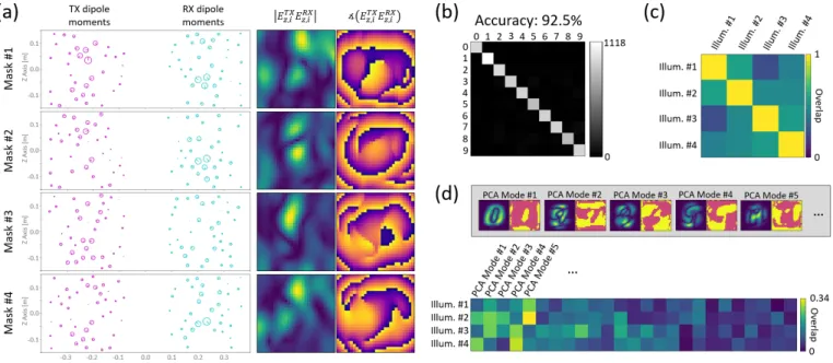
We begin by considering a single realization withM = 4 measurements andN = 64 metamaterial elements per metasurface. The dipole moments and scene illumina-tions corresponding to the four learned metasurface con-figurations are displayed in Fig. 3(a). The performance metric to evaluate the sensing ability is the average clas-sification accuracy on a set of 10,000 unseen samples. The confusion matrix in Fig. 3(b) specifically shows how often a given digit is classified by the ANN as one of the ten options. The strong diagonal (corresponding to correctly identified digits) reflects the achieved average accuracy of 92.5%. Note that the diagonal entries are not expected to be equally strong (e.g. the (1,1) entry is a bit stronger), since the test dataset does not include the exact same number of samples from each class. The off-diagonal entries of the confusion matrix are uniformly weak, so the ANN does not get particularly confused by any two classes.
We now study the sensing performance more system-atically for different values ofM andN. Since the ANN weights are initialized randomly before training, we con-duct 40 realizations for each considered parameter com-bination. Averaging over realizations allows us to focus on the role of M and N without being sensitive to a given realization. Moreover, we can see the extent to which different realizations converge to similar results. In Fig. 4(a) we contrast the sensing performance that we achieve by integrating a dynamic metasurface (con-sisting of 64 or 16 metamaterial elements) as physical layer into the ANN pipeline with the attainable perfor-mance if acquisition and processing are treated separately in schemes employing random, orthogonal or PCA-based scene illuminations.
Random illuminations yield the worst performance out of the four considered paradigms. Orthogonal illumi-nations yield a marginal improvement over random il-luminations as the number of measurements M gets larger, since the non-overlapping illuminations can ex-tract marginally more information about the scene. Yet the information that random and orthogonal illumina-tions encode in the measurements is not necessarily task-relevant. The PCA-based approach presents a notice-able performance improvement over generic illuminations but remains well below the attainable performance with learned optimal illumination settings obtained by inte-grating the analog layer into the ANN. Our LISP clearly outperforms the other three benchmarks. The PCA-based approach is quite sensitive to the number of tun-able elements in the dynamic metasurface (keeping the same aperture size), since beam synthesis works better
with more degrees of freedom. In contrast, using only 16 instead of 64 metamaterial elements yields almost iden-tical sensing performance if the dynamic metasurface is integrated into the ANN pipeline. This suggests that us-ing very few elements, and thus a very light hardware layer, our LISP can successfully perform sensing tasks.
ForM ≤5, our scheme yields gains in accuracy of the order of 10% which is a substantial improvement in the context of classification tasks [71]; for instance, automo-tive security, where the number of scene illuminations is very limited, would be enhanced significantly if the recog-nition of, say, a pedestrian on the road could be improved by 10%. The performance using our learned illumination settings saturates aroundM = 5 at 95%, meaning that we manage to extract all task-relevant information from a 28×28 scene with only 5 measurements. The compres-sion is enabled by the sparsity of task-relevant features in the scene. Yet our scene is not sparse in the canonical basis: our region of interest corresponds to the size of the metallic digits. Unlike traditional computational imag-ing schemes, the compression here comes from the dis-crimination between relevant and irrelevant information in a dense scene. Our LISP thus achieves a significant dimensionality reduction by optimally multiplexing task-relevant information from different parts of the scene in the analog layer. The dimensionality reduction brings about a double advantage with respect to timing con-straints: taking fewer measurements takes less time, and moreover less data has to be processed by the digital lay-ers. In our (not heavily optimized) ANN architecture, the computational burden of the first digital ANN layer is directly proportional to the number of measurements M. We thus believe that our scheme is very attractive in particular when real-time decisions based on wave-based sensing are necessary, notably in automotive security and touchless human-computer interaction. Moreover, a re-duced processing burden can potentially avoid the need to outsource computations from the sensor edge to cloud servers via wireless links, mitigating associated latency and security issues [72].
A natural question that arises (albeit irrelevant for practical applications) is whether the other benchmark illumination schemes (random, orthogonal, PCA-based) will eventually, using more measurements, be able to per-form as well as our LISP. For the N = 16 case, we thus evaluated the average classification accuracy also for M = N and M = 2N. Only the LISP curve had saturated; the other benchmarks accurracies were still slightly improving between M = N and M = 2N and were still somewhat below the LISP performance. Since the “scene illumination” Ii(ζ) = ETXi (ζ)·ERXi (ζ) de-pends on the configuration of two metasurfaces with N tunable elements each, we expect that all schemes per-form equally well only onceM ≥N2.
A striking difference in the performance fluctuations, evidenced by the error bars in Fig. 4(a), is also visible. While the performance of our LISP does not present any appreciable fluctuations forM ≥4, all other benchmark
8
FIG. 3. Analysis of LISP illumination patterns for a single realization with M = 4. (a) For each of the four masks, the corresponding TX and RX dipole moments, and the magnitude and phase of the corresponding scene illuminationsEz,iT XEz,iRX,
i∈ {1,2,3,4}, are shown. The dipole moment representations are as in the inset of Fig. 2. The magnitude maps are normalized individually, the phase maps have a colorscale from −π to π. (b) Confusion matrix evaluated on an unseen test dataset of 10,000 samples. This realization achieved 92.5% classification accuracy. (c) Mutual overlap of the four scene illuminations. The average over the off-diagonal entries of the overlap matrix is 0.45. (d) Overlap of the four scene illuminations with the first 25 PCA modes. Note that the colorscale’s maximum is 0.34 here (i.e. well below unity). The inset shows magnitude and phase of the first five PCA modes.
FIG. 4. (a) Comparison of the sensing performance with the LISP illumination settings with three benchmarks: random, orthogonal and PCA-based scene illuminations. (b) Analysis of the mutual overlap between distinct scene illumination. (c) Analysis of the maximum overlap of the scene illuminations with a PCA mode. All data points are averaged over 40 realizations. Errorbars indicate the standard deviation.
illumination schemes continue to fluctuate by several per-cent of classification accuracy. Our scheme’s performance is thus reliable whereas any of the other benchmarks in any given realization may (taking the worst-case sce-nario) yield a classification accuracy several percent be-low its average performance. Performance reliability of a sensor is important for deployment in real-life decision making processes.
B. Analysis of learned scene illuminations
The inferior performance of orthogonal and PCA-based illuminations suggests that the task-specific learned LISP illuminations do not trivially correspond neither to a set of optimally diverse illuminations nor to the principal components of the scene. To substantiate this observation, we go on to analyze the scene illumina-tions in more detail. First, within a given series of M illuminations, we compute the mutual overlap between different illuminations. In the following, we define the overlapOof two scene illuminationsA(ζ) andB(ζ) as
O(A, B) = R sceneA †B dζ q R sceneA†Adζ R sceneB†B dζ , (6)
where † denotes the conjugate transpose operation. An example overlap matrix forM = 4 is shown in Fig. 3(c). We define the illumination pattern overlap as the mean of the off-diagonal elements (the diagonal entries are unity by definition).
In Fig. 4(b) we present the average illumination pat-tern overlap for all four considered paradigms. For the case of orthogonal illuminations, the overlap is very close to zero, indicating that our inverse metasurface config-uration design worked well. The inverse design works considerably better withN = 64 as opposed toN = 16, and of course the more illuminations we want to be mu-tually orthogonal the harder the task becomes. While radiating orthogonal wavefronts with the dynamic meta-surface is not the best choice for sensing, it may well find applications in wireless communication [73]. For the case of random illuminations, the mutual overlap is constant at 28.5% and independent ofN. This is indeed the aver-age overlap of two random complex vectors of length 10, 10 corresponding roughly to the number of independent speckle grains in the scene — see Fig. 3(a).
The mutual overlap of PCA-based illuminations, ex-cept for very lowM, saturates around 21.5% and 24.5% for N = 64 and N = 16, respectively, and is hence lower than that of random illuminations. In principle, if beam synthesis worked perfectly, the PCA-based pat-terns should not overlap at all since PCA modes are or-thogonal by definition. The more degrees of freedom N we have, the better the beam synthesis works, and con-sequently the lower the mutual overlap of PCA-modes
is. For the LISP scene illuminations, the average mutual overlap is comparable to that of random scene illumina-tions. We hence conclude that the diversity of the scene illuminations is not a key factor for the extraction of task-relevant information.
Next, we investigate to what extent the scene illumina-tions overlap with PCA modes. An example of the over-lap with the first 25 PCA modes is provided in Fig. 3(d). In Fig. 4(c), we present the average of the maximum overlap that a given illumination pattern has with any of the PCA modes. For random and orthogonal illumi-nations, irrespective ofN andM, this overlap is around 20% and thus insignificant, as expected. For PCA-based illuminations we have performed beam synthesis to pre-cisely maximize this overlap. We achieve (65.0±1.9)% withN = 64 and (44.1±1.4)% withN = 16. The abil-ity to synthesize the PCA modes is thus very dependent on the number of metamaterial elements, and these re-sults demonstrate that the PCA-based approach is suit-able only for scenarios where N is large. This observa-tion is a further argument for the attractiveness of our approach in applications with very limited aperture size and tunability like automotive RADAR. In fact, since the PCA-based approach also requires an analytical forward model, one may as well choose the superior performance of our LISP proposal in any scenario where the PCA-based approach could be employed. Moreover, training with our approach is faster since all weights are optimized simultaneously, as opposed to first solvingM inverse de-sign problems and then training the digital weights.
The overlap of the LISP illuminations with PCA modes is around 30% and thus notably larger than for random or orthogonal illuminations but also notably lower than what can be achieved if one seeks PCA modes. Interest-ingly, the maximum overlap with a PCA mode is lower for M = 1 and M = 2. We conclude that the opti-mal illumination patterns identified by our ANN cannot simply be explained as corresponding to PCA modes, or to be a good approximation thereof. Notably for small M this is not the case. During training, the ANN finds an optimal compromise taking the inner workings of the nonlinear digital layers as well as the physical layer con-straints into account. The joint optimization of analog and digital layers provides substantially better perfor-mance than considering them separately and trying to anticipate useful illumination patterns.
We observe no significant difference in the performance across different metasurface realizations (i.e. different random locations of the metamaterial elements). The LISP scene illuminations overlap around 65% across dif-ferent realizations with the same metasurface, indicating that the optimization space contains numerous almost equivalent local minima. Remarkably, we never seem to get stuck in inferior local minima.
10
C. Robustness
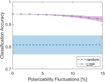
Finally, we investigate how robust the sensing perfor-mance is outside the nominal conditions, i.e. over a given set of parameter variations. Here, we consider variations of the metamaterial elements’ polarizability; due to fab-rication tolerances of electronic components such as the PIN diodes the experimental polarizability is expected to differ across metamaterial elements by a few percent from the value extracted via full-wave simulation based on the element’s design [3]. WithM = 5 andN = 64, we first train our LISP as before. Then, for each metamaterial element, we replace the true polarizability valueαyy by a differentα0yy =αyy(1 +), whereis white noise; real and imaginary parts ofare identically distributed with zero mean and standard deviationδ, so the standard de-viation of (the size of the cloud in the complex plane) is√2δ.
FIG. 5. Robustness of sensing performance to fluctuations in the metamaterial elements’ experimental polarizability. For a single realization with N = 64 and M = 5, the LISP is trained with the expected polarizability value. Then, its per-formance is evaluated after adding different amounts of white noise to the metamaterial elements’ polarizabilities. The pur-ple curve and shaded area indicate average and standard de-viation over 250 realizations of the polarizability fluctuations. For reference, the blue curve and shaded area indicate the av-erage performance with random metasurface configurations, see Fig. 4(a), which is independent of polarizability fluctua-tions since it does not rely on optimized wavefronts.
In Fig. 5 we display the dependence of the sensing per-formance of our LISP scheme as a function of the polar-izability fluctuations around the expected value. Mean and standard deviation over 250 realizations of fluctu-ations are shown in purple. Up to 5% of fluctufluctu-ations, the performance does not display any notable changes; around 10% a very slight degradation of the performance is observed. The benchmark for comparison here is the
case of using random illuminations since these do not rely on carefully shaped wavefronts and are thus not affected by experimental polarizability values different from the expected ones. Compared to the performance with ran-dom illuminations, our scheme is still clearly superior even for unrealistically high fluctuations on the order of 15%. These results suggest that realistic deviations from the expected polarizability values of the metamaterial el-ements, due to fabrication tolerances or other neglected effects, are by no means detrimental for our scheme.
V. OUTLOOK
In spite of the encouraging robustness results shown in the previous section IV C, it is worth considering how one would deal with significant fabrication inaccuracies in ex-perimental metasurfaces. Should one or several param-eters of the metasurface design, such as polarizabilities or locations of the metamaterial elements, turn out to significantly vary due to fabrication issues, an additional calibration step could easily learn the actual parameter values of a given fabricated metasurface. The spirit of this procedure is similar to the way in which we achieved beam synthesis (see Section B.3 of the Supplemental Ma-terial) using only the analog part of our pipeline. The parameters to be determined are declared as weight vari-ables to be learned during training and initialized with their expected values. Then experimentally the radiated fields for a few different metasurface configurations are measured and a cost function is defined to minimize dur-ing traindur-ing the difference between the measured and ex-pected radiated fields. By the end of the optimization, a set of parameter values will have been learned that opti-mally matches the experiment.
Furthermore, for practical applications it may be of in-terest to achieve a certain robustness to fluctuations in the calibration parameters such as geometrical details of the experimental setup [14, 74, 75]. By including ran-dom realizations of major calibration parameters within the expected range of fluctuation during the training, the network can learn to be invariant to these variations [14]. Ultimately, this enables the transfer of knowledge learned on synthesized data to real-life setups without additional training measurements. For a specific task such as hand gesture recognition, synthetic scenes can easily be gener-ated with appropriate 3D modelling tools.
In future implementations, it may be worthwhile to in-clude additional measurement and processing constraints in the LISP, such as phaseless measurements and few-bit processing [76], to lower the hardware requirements fur-ther. With more advanced forward models beyond the first Born approximation, quantitative imaging may be-come possible, for instance of the dielectric constant in contexts ranging from the detection of breast cancer to the inspection of wood [77, 78]. In practice, incremental learning techniques [79, 80] may enable one to adapt the LISP efficiently to new circumstances without retraining
from scratch, for instance if an additional class is to be recognized.
Finally, a conceptually exciting question for future re-search is how we can conceive a LISP that is capable of taking real-time on-the-fly decisions about the next opti-mal scene illumination, taking into account the available knowledge from previous measurements [81].
VI. CONCLUSION
In summary, we have shown that integrating the phys-ical layer of a wave-based sensor into its artificial-neural-network (ANN) pipeline substantially enhances the abil-ity to efficiently obtain task-relevant information about the scene. The jointly optimized analog and digital layers optimally encode relevant information in the measure-ments, converting data acquisition simultaneously into a first layer of data processing. A thorough analysis of the learned optimal illumination patterns revealed that they cannot be anticipated from outside the ANN pipeline, for instance by considerations to maximize the mutual in-formation or based on principal scene components, high-lighting the importance of optimizing a unique analog-digital pipeline.
As concrete example, we considered the use of dynamic metasurfaces for classification tasks which are highly rel-evant to emerging concepts of “context-awareness”, rang-ing from real-time decision makrang-ing in automotive secu-rity via gesture recognition for touchless human-device interactions to fall detection for smart health care of el-derly. The dynamic metasurfaces, thanks to their inher-ent analog multiplexing and structural compactness, are poised to play an important role in these applications.
Moreover, the sub-wavelength nature of the embedded metamaterial elements enabled us to formulate a very compact analytical forward model based on a coupled-dipole description that we then combined with the ma-chine learning framework of our Learned Integrated Sens-ing Pipeline. Several traditional inverse-design hurdles like binary constraints on the analog weights and cou-pling between metamaterial elements were cleared with ease in our scheme. In addition to a substantially higher classification accuracy, we observed that our scheme is more reliable (very low performance fluctuations across realizations) and very robust (against fabrication inaccu-racies).
The ability to very efficiently extract task-relevant in-formation greatly reduces the number of necessary mea-surements as well as the amount of the data to be pro-cessed by the digital layer, which is very valuable in the presence of strict timing constraints as found in most ap-plications. We expect our work to also trigger interesting developments in other areas of wave physics, notably op-tical and acoustic wavefront shaping [82, 83].
ACKNOWLEDGMENTS
M.F.I., A.V.D. and D.R.S. are supported by the Air Force Office of Scientific Research under award number FA9550-18-1-0187.
The project was initiated and conceptualized by P.d.H. with input from M.F.I. and R.H. The project was con-ducted and written up by P.d.H. All authors contributed with thorough discussions.
[1] P. Sebbah,Waves and Imaging through Complex Media
(Springer Science & Business Media, 2001).
[2] J. Hasch, E. Topak, R. Schnabel, T. Zwick, R. Weigel, and C. Waldschmidt, Millimeter-wave technology for au-tomotive radar sensors in the 77 GHz frequency band, IEEE Trans. Microw. Theory Tech.60, 845 (2012). [3] F. B. Khalid, D. T. Nugraha, A. Roger, and R. Ygnace,
Integrated target detection hardware unit for automotive radar applications, in 2017 European Radar Conference (EURAD)(IEEE, 2017) pp. 219–222.
[4] P. Rashidi and A. Mihailidis, A survey on ambient-assisted living tools for older adults, IEEE J. Biomed. Health Inform. 17, 579 (2013).
[5] F. Adib, H. Mao, Z. Kabelac, D. Katabi, and R. C. Miller, Smart homes that monitor breathing and heart rate, in
Proceedings of the 33rd Annual ACM Conference on Hu-man Factors in Computing Systems (ACM, 2015) pp. 837–846.
[6] P. Molchanov, S. Gupta, K. Kim, and K. Pulli, Multi-sensor system for driver’s hand-gesture recognition, in
2015 11th IEEE International Conference and Work-shops on Automatic Face and Gesture Recognition (FG),
Vol. 1 (IEEE, 2015) pp. 1–8.
[7] J. Lien, N. Gillian, M. E. Karagozler, P. Amihood, C. Schwesig, E. Olson, H. Raja, and I. Poupyrev, Soli: Ubiquitous gesture sensing with millimeter wave radar, ACM Transactions on Graphics (TOG)35, 142 (2016). [8] M. Sperrin and J. Winder, X-ray imaging, in Scientific
Basis of the Royal College of Radiologists Fellowship, 2053-2563 (IOP Publishing, 2014) pp. 2–1 to 2–50. [9] Y. Liu, P. Lai, C. Ma, X. Xu, A. A. Grabar, and L. V.
Wang, Optical focusing deep inside dynamic scattering media with near-infrared time-reversed ultrasonically en-coded (true) light, Nat. Commun.6, 5904 (2015). [10] D. Wang, E. H. Zhou, J. Brake, H. Ruan, M. Jang,
and C. Yang, Focusing through dynamic tissue with mil-lisecond digital optical phase conjugation, Optica2, 728 (2015).
[11] B. Blochet, L. Bourdieu, and S. Gigan, Focusing light through dynamical samples using fast continuous wave-front optimization, Opt. Lett.42, 4994 (2017).
[12] C. Katrakazas, M. Quddus, W.-H. Chen, and L. Deka, Real-time motion planning methods for autonomous on-road driving: State-of-the-art and future research
direc-12
tions, Transportation Research Part C: Emerging Tech-nologies60, 416 (2015).
[13] A. Krizhevsky, I. Sutskever, and G. E. Hinton, Imagenet classification with deep convolutional neural networks, in Advances in Neural Information Processing Systems
(2012) pp. 1097–1105.
[14] G. Satat, M. Tancik, O. Gupta, B. Heshmat, and R. Raskar, Object classification through scattering media with deep learning on time resolved measurement, Opt. Express25, 17466 (2017).
[15] A. Sinha, J. Lee, S. Li, and G. Barbastathis, Lensless computational imaging through deep learning, Optica4, 1117 (2017).
[16] Y. Rivenson, Z. G¨or¨ocs, H. G¨unaydin, Y. Zhang, H. Wang, and A. Ozcan, Deep learning microscopy, Op-tica4, 1437 (2017).
[17] N. Borhani, E. Kakkava, C. Moser, and D. Psaltis, Learning to see through multimode fibers, Optica5, 960 (2018).
[18] Y. Li, Y. Xue, and L. Tian, Deep speckle correlation: a deep learning approach toward scalable imaging through scattering media, Optica5, 1181 (2018).
[19] G. Montaldo, D. Palacio, M. Tanter, and M. Fink, Building three-dimensional images using a time-reversal chaotic cavity, IEEE Trans. Ultrason. Ferroelectr. Freq. Control52, 1489 (2005).
[20] W. L. Chan, K. Charan, D. Takhar, K. F. Kelly, R. G. Baraniuk, and D. M. Mittleman, A single-pixel tera-hertz imaging system based on compressed sensing, Appl. Phys. Lett.93, 121105 (2008).
[21] J. Hunt, T. Driscoll, A. Mrozack, G. Lipworth, M. Reynolds, D. Brady, and D. R. Smith, Metamate-rial apertures for computational imaging, Science 339, 310 (2013).
[22] A. Liutkus, D. Martina, S. Popoff, G. Chardon, O. Katz, G. Lerosey, S. Gigan, L. Daudet, and I. Carron, Imag-ing with nature: Compressive imagImag-ing usImag-ing a multiply scattering medium, Sci. Rep.4, 5552 (2014).
[23] A. J. Fenn, D. H. Temme, W. P. Delaney, and W. E. Courtney, The development of phased-array radar tech-nology, Lincoln Laboratory Journal12, 321 (2000). [24] R. D. Swift, R. B. Wattson, J. A. Decker, R. Paganetti,
and M. Harwit, Hadamard transform imager and imaging spectrometer, Appl. Opt.15, 1595 (1976).
[25] C. M. Watts, D. Shrekenhamer, J. Montoya, G. Lipworth, J. Hunt, T. Sleasman, S. Krishna, D. R. Smith, and W. J. Padilla, Terahertz compressive imaging with metamate-rial spatial light modulators, Nat. Photon.8, 605 (2014). [26] G. Satat, M. Tancik, and R. Raskar, Lensless imaging with compressive ultrafast sensing, IEEE Trans. Comput. Imag.3, 398 (2017).
[27] I. Jolliffe, Principal Component Analysis (Springer, 2011).
[28] M. A. Neifeld and P. Shankar, Feature-specific imaging, Appl. Opt.42, 3379 (2003).
[29] M. Liang, Y. Li, H. Meng, M. A. Neifeld, and H. Xin, Reconfigurable array design to realize principal compo-nent analysis (PCA)-based microwave compressive sens-ing imagsens-ing system, IEEE Antennas Wirel. Propag. Lett.
14, 1039 (2015).
[30] L. Li, H. Ruan, C. Liu, Y. Li, Y. Shuang, A. Al`u, C.-W. Qiu, and T. J. Cui, Machine-learning reprogrammable metasurface imager, Nat. Commun.10, 1082 (2019). [12] A. Chakrabarti, Learning sensor multiplexing design
through back-propagation, inAdvances in Neural Infor-mation Processing Systems (2016) pp. 3081–3089. [32] R. Horstmeyer, R. Y. Chen, B. Kappes, and B.
Judke-witz, Convolutional neural networks that teach micro-scopes how to image, arXiv preprint arXiv:1709.07223 (2017).
[24] T. Sleasman, M. F. Imani, J. N. Gollub, and D. R. Smith, Dynamic metamaterial aperture for microwave imaging, Appl. Phys. Lett.107, 204104 (2015).
[25] M. F. Imani, T. Sleasman, and D. R. Smith, Two-dimensional dynamic metasurface apertures for com-putational microwave imaging, IEEE Antennas Wirel. Propag. Lett.17, 2299 (2018).
[5] T. Sleasman, M. F. Imani, W. Xu, J. Hunt, T. Driscoll, M. S. Reynolds, and D. R. Smith, Waveguide-fed tun-able metamaterial element for dynamic apertures, IEEE Antennas Wirel. Propag. Lett.15, 606 (2016).
[36] A. Silva, F. Monticone, G. Castaldi, V. Galdi, A. Al`u, and N. Engheta, Performing mathematical operations with metamaterials, Science343, 160 (2014).
[37] T. Zhu, Y. Zhou, Y. Lou, H. Ye, M. Qiu, Z. Ruan, and S. Fan, Plasmonic computing of spatial differentiation, Nat. Commun.8, 15391 (2017).
[38] Y. Shen, N. C. Harris, S. Skirlo, M. Prabhu, T. Baehr-Jones, M. Hochberg, X. Sun, S. Zhao, H. Larochelle, D. Englund,et al., Deep learning with coherent nanopho-tonic circuits, Nat. Photon.11, 441 (2017).
[39] P. del Hougne and G. Lerosey, Leveraging chaos for wave-based analog computation: Demonstration with indoor wireless communication signals, Phys. Rev. X8, 041037 (2018).
[40] N. M. Estakhri, B. Edwards, and N. Engheta, Inverse-designed metastructures that solve equations, Science
363, 1333 (2019).
[41] T. W. Hughes, I. A. D. Williamson, M. Minkov, and S. Fan, Wave physics as an analog recurrent neural net-work, arXiv preprint arXiv:1904.12831 (2019).
[42] F. Zangeneh-Nejad and R. Fleury, Topological analog sig-nal processing, Nat. Commun.10, 2058 (2019).
[43] D. Pierangeli, G. Marcucci, and C. Conti, Large-scale photonic ising machine by spatial light modulation, Phys. Rev. Lett.122, 213902 (2019).
[1] L. Pulido-Mancera, M. F. Imani, P. T. Bowen, N. Kundtz, and D. R. Smith, Analytical modeling of a two-dimensional waveguide-fed metasurface, arXiv preprint arXiv:1807.11592 (2018).
[2] G. Lipworth, A. Rose, O. Yurduseven, V. R. Gowda, M. F. Imani, H. Odabasi, P. Trofatter, J. Gollub, and D. R. Smith, Comprehensive simulation platform for a metamaterial imaging system, Appl. Opt. 54, 9343 (2015).
[6] Separating the metamaterial elements by at least one free-space wavelengths avoids evanescent coupling be-tween them.
[47] R. Guzman-Quiros, J. L. Gomez-Tornero, A. R. Weily, and Y. J. Guo, Electronic full-space scanning with 1-D Fabry–P´erot LWA using electromagnetic band-gap, IEEE Antennas Wirel. Propag. Lett.11, 1426 (2012).
[48] J.-H. Fu, A. Li, W. Chen, B. Lv, Z. Wang, P. Li, and Q. Wu, An electrically controlled CRLH-inspired cir-cularly polarized leaky-wave antenna, IEEE Antennas Wirel. Propag. Lett16, 760 (2017).
[49] K. Chen, Y. H. Zhang, S. Y. He, H. T. Chen, and G. Q. Zhu, An Electronically Controlled Leaky-Wave
Antenna Based on Corrugated SIW Structure With Fixed-Frequency Beam Scanning, IEEE Antennas Wirel. Propag. Lett18, 551 (2019).
[50] J. Huang and J. A. Encinar,Reflectarray Antennas(John Wiley & Sons, 2008).
[51] D. Sievenpiper, J. Schaffner, R. Loo, G. Tangonan, S. On-tiveros, and R. Harold, A tunable impedance surface per-forming as a reconfigurable beam steering reflector, IEEE Trans. Antennas Propag.50, 384 (2002).
[52] T. J. Cui, M. Q. Qi, X. Wan, J. Zhao, and Q. Cheng, Coding metamaterials, digital metamaterials and pro-grammable metamaterials, Light Sci. Appl. 3, e218 (2014).
[53] S. Lim, C. Caloz, and T. Itoh, Metamaterial-based electronically controlled transmission-line structure as a novel leaky-wave antenna with tunable radiation angle and beamwidth, IEEE Trans. Microw. Theory Tech.52, 2678 (2004).
[54] D. J. Gregoire, J. S. Colburn, A. M. Patel, R. Quarfoth, and D. Sievenpiper, A low profile electronically-steerable artificial-impedance-surface antenna, in 2014 Interna-tional Conference on Electromagnetics in Advanced Ap-plications (ICEAA) (2014) pp. 477–479.
[55] B. T. Draine and P. J. Flatau, Discrete-dipole approx-imation for scattering calculations, J. Opt. Soc. Am. A
11, 1491 (1994).
[56] A. D. Scher and E. F. Kuester, Extracting the bulk ef-fective parameters of a metamaterial via the scattering from a single planar array of particles, Metamaterials3, 44 (2009).
[57] P. T. Bowen, T. Driscoll, N. B. Kundtz, and D. R. Smith, Using a discrete dipole approximation to predict com-plete scattering of complicated metamaterials, New J. Phys.14, 033038 (2012).
[58] N. Landy and D. R. Smith, Two-dimensional metamate-rial device design in the discrete dipole approximation, J. Appl. Phys.116, 044906 (2014).
[59] M. Dupr´e, P. del Hougne, M. Fink, F. Lemoult, and G. Lerosey, Wave-field shaping in cavities: Waves trapped in a box with controllable boundaries, Phys. Rev. Lett.115, 017701 (2015).
[60] P. del Hougne, F. Lemoult, M. Fink, and G. Lerosey, Spatiotemporal wave front shaping in a microwave cavity, Phys. Rev. Lett.117, 134302 (2016).
[61] T. Sleasman, M. F. Imani, J. N. Gollub, and D. R. Smith, Microwave imaging using a disordered cavity with a dy-namically tunable impedance surface, Phys. Rev. Appl.
6, 054019 (2016).
[22] J. Peurifoy, Y. Shen, L. Jing, Y. Yang, F. Cano-Renteria, B. G. DeLacy, J. D. Joannopoulos, M. Tegmark, and M. Soljaˇci´c, Nanophotonic particle simulation and in-verse design using artificial neural networks, Sci. Adv.
4, eaar4206 (2018).
[23] D. Liu, Y. Tan, E. Khoram, and Z. Yu, Training deep neural networks for the inverse design of nanophotonic structures, ACS Photonics5, 1365 (2018).
[3] L. Pulido-Mancera, P. T. Bowen, M. F. Imani, N. Kundtz, and D. Smith, Polarizability extraction of complementary metamaterial elements in waveguides for aperture modeling, Phys. Rev. B96, 235402 (2017). [9] We work with identical metamaterial elements here but
note that the formalism can deal with different polariz-abilities for different elements, see also Section IV C. [66] A detailed discussion on effective polarizability and the
self-interaction term of the Green’s function can be found in Section II of Ref. [3].
[29] J. D. Jackson, Classical Electrodynamics (New York: John Wiley & Sons., 1975).
[68] Each measurement corresponds to a distinct pair of a TX and an RX pattern. This is different from previ-ous computational imaging schemes with random meta-surface configurations [25] that defined a set of random configurations and took a measurement for each possible combination of TX and RX configurations within the set. [69] P. del Hougne, M. F. Imani, M. Fink, D. R. Smith, and G. Lerosey, Precise localization of multiple noncoopera-tive objects in a disordered cavity by wave front shaping, Phys Rev. Lett.121, 063901 (2018).
[11] D. E. Rumelhart, G. E. Hinton, and R. J. Williams, Learning representations by back-propagating errors, Na-ture323, 533 (1986).
[71] A. Krizhevsky, I. Sutskever, and G. E. Hinton, Imagenet classification with deep convolutional neural networks, in Advances in Neural Information Processing Systems
(2012) pp. 1097–1105.
[72] M. M. Hossain, M. Fotouhi, and R. Hasan, Towards an analysis of security issues, challenges, and open problems in the internet of things, in2015 IEEE World Congress on Services (IEEE, 2015) pp. 21–28.
[73] P. del Hougne, M. Fink, and G. Lerosey, Optimally diverse communication channels in disordered environ-ments with tuned randomness, Nat. Electron. 2, 36 (2019).
[74] A. Mutapcic, S. Boyd, A. Farjadpour, S. G. Johnson, and Y. Avniel, Robust design of slow-light tapers in periodic waveguides, Eng. Optimiz.41, 365 (2009).
[75] M. Sniedovich, From statistical decision theory to robust optimization: A maximin perspective on robust decision-making, inRobustness Analysis in Decision Aiding, Op-timization, and Analytics (Springer, 2016) pp. 59–87. [76] V. Sze, Y.-H. Chen, T.-J. Yang, and J. S. Emer,
Effi-cient processing of deep neural networks: A tutorial and survey, Proc. IEEE105, 2295 (2017).
[77] E. C. Fear, X. Li, S. C. Hagness, and M. A. Stuchly, Confocal microwave imaging for breast cancer detection: Localization of tumors in three dimensions, IEEE Trans. Biomed. Eng.49, 812 (2002).
[78] F. Boero, A. Fedeli, M. Lanini, M. Maffongelli, R. Mon-leone, M. Pastorino, A. Randazzo, A. Salvad`e, and A. Sansalone, Microwave tomography for the inspection of wood materials: Imaging system and experimental results, IEEE Trans. Microw. Theory Tech. 66, 3497 (2018).
[79] J. Yoon, E. Yang, J. Lee, and S. J. Hwang, Lifelong learning with dynamically expandable networks, arXiv preprint arXiv:1708.01547 (2017).
[80] F. M. Castro, M. J. Mar´ın-Jim´enez, N. Guil, C. Schmid, and K. Alahari, End-to-end incremental learning, in Pro-ceedings of the European Conference on Computer Vision (ECCV)(2018) pp. 233–248.
[81] V. Mnih, N. Heess, A. Graves, and K. Kavukcuoglu, Re-current models of visual attention, inAdvances in Neural Information Processing Systems(2014) pp. 2204–2212. [82] S. Rotter and S. Gigan, Light fields in complex media:
Mesoscopic scattering meets wave control, Rev. Mod. Phys.89, 015005 (2017).
[83] G. Ma, X. Fan, P. Sheng, and M. Fink, Shaping reverber-ating sound fields with an actively tunable metasurface,
14
SUPPLEMENTAL MATERIAL
For the interested reader, here we provide numerous additional details that complement the manuscript and provide further illustrations. This document is organized as follows:
A. Detailed Description of the Physical Layer.
1. Dipole Moments for Array of Interacting Dipoles. 2. Visualization of Dipole Interaction.
3. Tuning Mechanism. 4. Propagation to Scene.
B. Details of Artificial Neural Network Algorithm and Parameters.
1. Training Algorithm and Parameters.
2. Imposing a Discrete Distribution of Weights. 3. Constrained Beam Synthesis / Wavefront Shap-ing.
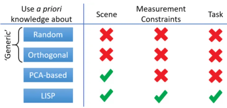
C. Taxonomy of Illumination Strategies in Wave-Based Sensing.
A. Detailed Description of the Physical Layer
In this section we provide, for completeness, the equa-tions used (i) to compute the dipole moments and (ii) to describe the propagation to the scene. We refer the inter-ested reader to Ref. [1] and Ref. [2], respectively, where these expression are derived in a more general form.
1. Dipole Moments for Array of Interacting Dipoles
The goal of this section is to compute the dipole mo-ments of each radiating element for a given configuration to then use them to compute the radiated field in the scene as detailed in Section VI A 4.
The metamaterial elements can be described as mag-netic dipoles due to their small size compared to the wavelength. Using surface equivalent principles [3], an equivalent polarizability tensor αfor a given metamate-rial element can be extracted. The metamatemetamate-rial’s dipole momentmis then determined as
m(r) =αHloc(r), (S1)
where Hloc is the local field at the metamaterial’s posi-tionr.
For the example metamaterial element shown in the inset of Fig. 1(a) in the main text (a tunable cELC-resonator [4, 5]), at the working frequency off0= 10 GHz (wavelength λ0 = 0.03 m), only the αyy component of the polarizability tensor is significant [1]. This simplifies Eq. S1 to
my(r) =αyy Hyloc(r) (S2)
for the setup we consider.
The crux now lies in computing the local fieldHloc y (r) exciting a given metamaterial element. Hloc
y (r) is a su-perposition of the cylindrical wave feeding the waveguide, Hf eed
y (r), and the fields Hyinteract(r) radiated from the other metamaterial elements:
Hyloc(r) =Hyf eed(r) +Hyinteract(r). (S3)
The analytical expression for Hf eed
y (r) reads
Hyf eed(r) = iIek
4 H
(2)
1 (k|r−r0|) sin(θ), (S4) where i is the imaginary unit,Ieis the amplitude of the electric line source generating the feed wave (taken to be 1 A in the following),k= 2πf0/cis the propagation constant of the fundamental mode inside the waveguide, H(2)1 is a first order Hankel function of the second kind,r0 is the position of the source, andθ is the circumferential angle around the source measured from they-axis. The space inside the waveguide we consider is empty (not filled with a substrate).
The fieldHyinteract(ri) exciting theith dipole due to the presence of other dipoles can be related to the Green’s functionGyy(ri,rj) between the element under consider-ation at position ri and the jth element at position rj as
Hyinteract(ri) =
X
i6=j
Gyy(ri,rj)my(rj). (S5)
The self-interaction term, i.e. i=j, is included in the definition of effective polarizability, as detailed in Sec-tion II of Ref. [3]. Note that Eq. S2 and Eq. S5 are coupled via themy(rj) term. To compute the dipole mo-mentsmy(rj), we thus have to solve a system of coupled equations. First, rearranging both to yield an expression forHyloc(ri) yields
Hyloc(ri) =α−1yy my(ri), (S6a)
Hyloc(ri) =Hyf eed(ri) +
X
i6=j
Gyy(ri,rj)my(rj). (S6b)
Next, we rewrite Eq. S6 in matrix form:
AM=F+GM, (S7)
whereAis a diagonal matrix whose diagonal entries are α−1yy (all metamaterial elements are identical), M is a vector containing the sought-after dipole moments,Gis a matrix whose entry (i, j) corresponds to the Green’s
16
function between elements at positions ri and rj (the diagonal entries are set to zero since the self-interaction terms are incorporated into the effective polarizabilities in A), andFis a vector containing the fields due to the feeding wave at the element positions.
Solving Eq. S7 forM then yields
M={A−G}−1F. (S8)
Now, the remaining step is to identify an expression for the inter-element Green’s function Gyy(ri,rj). The inter-element coupling consists of two components — in-teractions via the waveguide (WG) and inin-teractions via free space (FS):
Gyy(ri,rj) =GW Gyy (ri,rj) +GF Syy (ri,rj). (S9) The waveguide interaction component reads
GW Gyy (ri,rj) =− ik2 8h H(2)0 (kR)−cos(2φ) H(2)2 (kR), (S10) whereR=|ri−rj|andφis the angle of the vector from
ri torj. The free space interaction [? ] is given by
GF Syy (ri,rj) =g(R) k2+ ik R − 1 +k2∆2 y R2 − 3ik∆2 y R3 + 3∆2 y R4 ! , (S11) where ∆y =yi−yj andg(R) = 2e4πR−ikR. The factor 2 in the expression forg(R) originates from self-images of the elements due to the waveguide’s metallic upper plate.
2. Visualization of Dipole Interaction
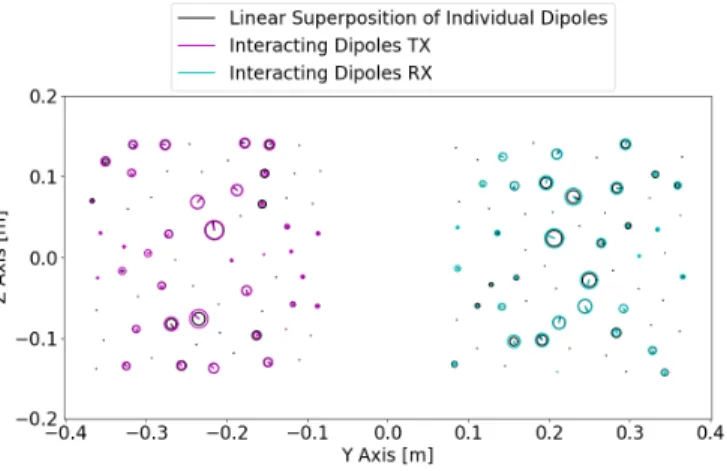
In this section we provide a visualization of the impor-tance of accounting for the coupling between different metamaterial elements. To that end, we first compute for a random configuration of the metasurface shown in Fig. 1(a) of the main text the corresponding dipole mo-ments for each metamaterial element. We compare this with a linear superposition of the individual elements, i.e. omitting the presence of other dipoles in calculating each element’s dipole moment.
The comparison in Fig. S1 clearly shows the non-negligible difference between the two results, highlighting the importance of accounting for the coupling between metamaterial elements.
3. Tuning Mechanism
So far, the above calculations are for a device that is not reconfigurable, i.e. all included dipoles are radi-ating energy. For our scheme based on reconfigurabil-ity it is hence crucial to add a description of the tuning
FIG. S1. Comparison of the dipole momentsmy computed
for each metamaterial element, without (black) and with (pur-ple/cyan) accounting for the coupling between elements. The dipole moments are represented as phasors, with the radius of the circle being proportional to their amplitude, and the line segment showing their phase. The circles are centered on the physical location of each metamaterial element.
mechanism. Any phase or amplitude tuning is relative to the element’s polarizabilityαyy; for instance, the tuning states “on” and “off” that are accessible with a metama-terial element tuned via PIN-diodes connected across the cELC’s capacitive gaps [5] correspond to multiplying the polarizability by 1 or 0. If the polarizability is zero, the element is not radiating any energy and is hence essen-tially non-existant. This simple picture neglects ohmic losses associated with the PIN diodes when they are in conducting mode (i.e. the metamaterial element is not radiating); these losses are usually small but could be accounted for in any given practical implementation.
Consider a general tuning state described via a vector
T whose jth entry tj corresponds to the tuning of the jth element. The element’s polarizability is thentjαyy. Correspondingly, the jth diagonal entry of A becomes
{tjαyy}−1. In practice, to avoid issues related to division by zero, we use{tjαyy+δ}−1withδbeing four orders of magnitude smaller thanαyy.
A simple sanity check to confirm the above procedure consists in computing the magnetic dipole moments cor-responding to a binary (random) configuration T and comparing the result to that obtained if elements in the “off” state are simply omitted. Ideally the same magnetic dipole moments are computed for the “on” elements in both cases. This is indeed the case, as shown in Fig. S2.
4. Propagation to Scene
Having found a description of the transceiver ports in terms of dipole clusters, we can now proceed with com-puting the fields illuminating the scene for a given choice of physical layer weights. The considered setup is shown