TECHNICAL UNIVERSITY OF CLUJ-NAPOCA
ACTA TECHNICA NAPOCENSIS
Series: Applied Mathematics, Mechanics, and Engineering Vol. 61, Issue II, June, 2018
EVALUATING THE INFLUENCE OF THE PARAMETERS THAT
CHARACTERIZE THE TRAFFIC INCIDENTS BY USING THE
SENSITIVITY ANALYSIS OF THE OBTAINED RESULTS
Adrian TODORUŢ, Nicolae CORDOŞ, Monica BĂLCĂU, Alexandru TOACĂ
Abstract: This paper analyses the possibilities available for the reconstruction of the retrospective stages of road incidents of a vehicle-vehicle type, by following the evaluation of the velocities before the collision and determining the influence of certain parameters on the obtained results. A fist case study we modified the angle before the collision of a vehicle involved in an incident and we observed its influence on the velocity before the collision. The second case study modified the mass of one of the vehicles and we observed its influence on the velocity before the collision. The main reasons for choosing these two parameters as variables are: the angle before the collision can be changed by the driver without knowing by observing a potential incident situation, in an attempt to avoid the collision; we chose changing the mass of one of the vehicles because it is very seldom that studies take into account the real mass of the vehicle, most of the times the reports take into account the own mass of the vehicle or its total mass, according to the technical specifications. Given the fact that the reconstruction of the stages of traffic incidents are done with the help of conservation of energy, one can use one of the most used methods, namely the method of conservation of energy and the method of conservation of momentum. Thus, taking into account the physical models of the traffic incidents studied, based on the method of conservation of momentum and using mathematical modelling, we can calculate the velocities before the collision of the vehicles. In this respect, we studied two traffic incidents. Because the initial data were based on schematics taken at the site, testimonials, etc., we studied various methods for uncertainty analysis. We studied the level of confidence of the results obtained and a sensitivity analysis of certain variable parameters, thus identifying an interval for the output data, that is, the velocities before the collision with a certain degree of certainty.
Key words: vehicle, velocity, traffic incident, numerical modelling, uncertainty analysis, sensitivity analysis
1. INTRODUCTION
The issue of uncertainty is an important one when retrospectively reconstructing traffic incidents and it can be used either by means of the uncertainty analysis of the results or by the sensitivity analysis of a parameter [1-8]. In order to evaluate the uncertainty of an analysis, we notice that we can apply various numerical methods. The sensitivity analysis represents an analysis that would validate the applied method that modifies the values of one or more variables in order to observe how those specific changes the final results. If an analysis is strongly sensitive to one or more variables, then the confidence level in the final results decreases
and so the span of the final values must be increased.
This theme is dealt with in several papers that describe a variety of complex analysis methods [1-10].
Paper [2] used the Monte Carlo Analysis (MCA) to evaluate the velocities pre-collision of the vehicles involved in a traffic incident and the probabilities that the velocities might have been affected by the incident itself.
Paper [5] captured a comparison between various sensitivity analyses with reference to the mathematical, statistical or graphical methods. Many times, the sensitivity analyses aim to represent graphically the results so that they can show the individual influence of each input parameter on the obtained results, but if the sensitivity between two parameters varies significantly, their dependencies cannot always be graphically represented [5].
When the vehicles involved in a traffic incident present a significant difference of momentum, due to the considerable difference in their velocities or their masses, then [7] any slight change in the angles pre or post collision of one of the vehicles (usually the heaviest one), considerably affects the calculated velocity for the other vehicle. Thus, the sensitivity shows the importance of each variable of the method, in the sense of how or how much the final results change, and this helps the specialists to reconstruct the traffic incidents and establish which parameters need additional and more precise measurements.
In the case of the uncertainty analysis, several methods can be used [7, 8] that aim to determine the so called confidence interval for the results obtained. This confidence interval is needed because the values used to determine certain parameters (for example the pre-collision velocities) have a certain degree of uncertainty caused by certain errors, which does not allow to determine dot to dot calculations. In this case, the maximal and minimal values for the measurement variations need to be determined.
This paper used the sensitivity analysis to demonstrate the influence of a single parameter on the results obtained in the case of the two vehicle collision incident. In the first example we varied the pre-collision angle of the second vehicle involved in the incident. In the case of the second example presented in the paper, we suggested changing the mass of the first vehicle from the own mass to its total.
2. THE NUMERICAL EVALUATION METHOD
The first example in the present study, we changed the pre-collision angle for the second vehicle involved in the traffic incident, this being ±5° from the initial value. When increasing the angle between the longitudinal axis of the second vehicle and the referential axis, the angle between the two vehicles will also increase. We chose to change the angle because a ±5° change of the position of the vehicle is hardly noticeable by the human eye. This change in the position of the vehicle can be caused by the driver’s reflexes by instinctively turning the steering wheel in order to avoid the collision. Thus, we observe the influence of this instinct over avoiding the accident and over the consequences caused by the traffic incident. In the other example, we aimed to change the mass of the first vehicle, from its own mass all the way to the total mass, thus observing the influence of the mass of one of the vehicles on the velocities of each of the parties involved in the incident.
The research takes into account the collision of two vehicles taking into account their position in the pre- collision and post collision phases, which demands choosing the referential axes Ox and Oy. The referential axis Ox is to have the same direction and vector as the pre-collision velocity of one of the vehicles involved in the incident, thus the angle α formed
2 x 2 1 e 2 1 ) x (
f
σ µ − ⋅ −
⋅ π ⋅ ⋅ σ
= , (1)
where: x is the random variable of a statistical population; µ – average value; σ – standard
variation.
2.1. Evaluating the influence of the pre-collision angle changing
Let’s take a traffic incident with two vehicles involved (BMW e38 and Mercedes-Benz W124). Figure 1 represents schematically the pre and post collision positions of the vehicles involved in the incident, at table 1 presents the initial data needed to calculate the pre-collision velocities of the vehicles involved in the traffic incident.
In order to calculate the pre-collision velocities, we use the relations [2, 3]:
α ⋅
β ⋅ ⋅ − ϕ ⋅ ⋅ + θ ⋅ ⋅ =
cos m
cos v m cos v m cos v m v
1
2 2 4
2 3
1
1 , (2)
β ⋅
α ⋅ ⋅ − ϕ ⋅ ⋅ + θ ⋅ ⋅ =
sin m
sin v m sin v m sin v m v
2
1 1 4
2 3
1
2 . (3)
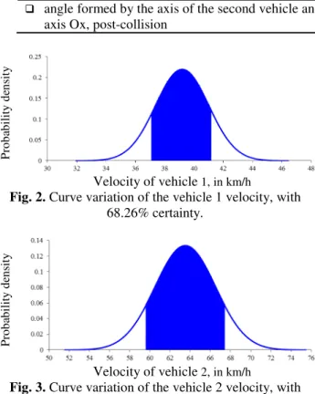
For the uncertainty analysis of the pre-collision angle, by using the data in table 1 and relations (2) and (3), we get velocities: v1 = 39.195 km/h, v2 = 63.518 km/h. For a
degree of certainty of 68.26%, the pre-collision velocity vehicle 1 is 39.195±1.811 km/h (Fig. 2) and the pre-collision velocity of vehicle 2 is 63.518±2.993 km/h (Fig. 3).
In the case of 95.45% certainty, the pre-collision velocity of the first vehicle is 39.195±3.623 km/h and the pre-collision velocity of the second vehicle is 63.518±5.99 km/h. For a certainty of 99.73% the pre-collision velocity of the first vehicle is 39.195±5.434 km/h and the pre-collision velocity of the second vehicle is 63.518±8.993 km/h.
Table 1 Input data for the evaluation of the influence for the pre-collision angle changes
Parameter Mark Value U.M.
mass for the first vehicle m1 2410 kg
mass for the second vehicle m2 1680 kg
post-collision velocity for the first vehicle v3 35 km/h
post-collision velocity for the second vehicle v4 35 km/h
angle formed by the axis of the first vehicle and the referential
axix Ox, pre-collision α 0 deg
angle formed by the axis of the second vehicle and the referential
axis Ox, pre-collision β 90 deg
angle formed by the axis of the first vehicle and the referential
axis Ox, post-collision θ 53 deg
angle formed by the axis of the second vehicle and the referential
axis Ox, post-collision φ 42 deg
P
ro
ba
bi
li
ty
d
en
si
ty
Velocity of vehicle 1, in km/h
Fig. 2. Curve variation of the vehicle 1 velocity, with 68.26% certainty.
P
ro
ba
bi
li
ty
d
en
si
ty
Velocity of vehicle 2, in km/h
Fig. 3. Curve variation of the vehicle 2 velocity, with 68.26% certainty.
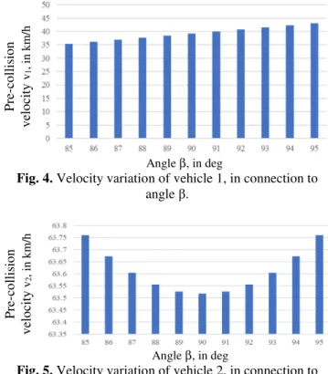
For the sensitivity analysis of the pre-collision angle of the pre-collision velocities, we used relations 2 and 3, where the value β was
modified from 85° to 95°. The results of the calculations for the pre-collision velocities are depicted in figure 4 (for vehicle 1) and figure 5 (for vehicle 2).
From figure 4 we can notice a linear increase in the pre-collision velocity of the first vehicle when the pre-collision angle β increases for the
second vehicle, meaning they are directly proportional. Thus, the higher the angle between these vehicles, the higher the need for a higher velocity for vehicle 1 in order to obtain post-collision velocities and angles similar to the
post-collision velocities and angles similar to the ones in the studied example. As a consequence, we can assume that the higher the β angle is
higher in collision, the higher the energy dissipated through the plastic deformation of the vehicles involved in the traffic incident.
The variation of the pre-collision velocity according to the pre-collision angle for the second vehicle (Figure 5) has the shape of a convex parable, given the fact that the value of the sinus of this angle varies in the form of a concave curve, whose values vary within the interval [-1, 1]. The value of the sinus is a part of the denominator of function velocity, thus the curve changing the shape from concave to convex.
According to the results obtained, in the case of the collisions where the pre-collision angles of one of the vehicle other than 90°, the energy dissipated by plastic deformation is higher than in the case of collisions under a pre-collision angle of 90°. At an angle variation of ±5° from the studied case, the energy consumed by the plastic deformation is insignificant, the velocity changes with about 0.3 km/h. By a simple mathematical calculation, if the given angle is 0°, the post-collision velocity would drop with about 5 km/h, which is of insignificant value.
P
re
-c
ol
li
si
on
ve
lo
ci
ty
v1
, i
n
km
/h
Angle β, in deg
Fig. 4. Velocity variation of vehicle 1, in connection to angle β.
P
re
-c
ol
li
si
on
ve
lo
ci
ty
v2
, i
n
km
/h
Angle β, in deg
Fig. 5. Velocity variation of vehicle 2, in connection to angle β.
2.2. Evaluating the influence of the vehicle mass changing
For this case, we took into account a traffic incident with two vehicles involved (Lexus GS300 - vehicle 1, with mass m1 and Audi A8 -
vehicle 2, with mass m2). The first vehicle was
to position itself on the first lane after coming out of the junction. During this manoeuvre, it came in collision with vehicle 2, which was holding precedence (Fig. 6). We know the pre and post collision angles, and the post-collision velocities. The known values from the incident site are presented in table 2, and with the
relations (2) and (3), we can determine the pre-collision velocities of the vehicles, thus obtaining v1 = 47.43 km/h and v2 = 42.52 km/h.
For the uncertainty analysis of the mass of the vehicle, the calculation of the confidence interval of the pre-collision velocity is similar to the first case studied. With a certainty of 68.26%, when the standard variation is considered just one σ, the confidence interval of
the pre-collision velocity for the first vehicle is v1 = 47.43±2.952 km/h (Fig. 7) and for the
second one is v2 = 42.52±2.03 km/h (Fig. 8).
For a certainty of 95.45% the variation for each velocity increases, because the uncertainty interval increases from one σ to 2⋅σ. Thus, we
get v1 = 47.43±5.876 km/h, respectively
v2 = 42.52±4.06 km/h. By increasing the
standard variation interval from 2σ to 3σ, the
credibility also increases to 99.73%, thus also increasing the interval of the pre-collision velocities of the vehicles v1 = 47.43±8.774 km/h,
respectively v2 = 42.52±6.09 km/h.
For the sensitivity analysis of the mass of the vehicle, we will take into account the fact that the mass of the first vehicle will vary from its own mass to the total mass of the vehicle according to the technical specs. So the aim is to observe the influence of the mass of one vehicle over the velocity of each participant at traffic incident.
Figure 9 captures the variation of the velocity for the first vehicle according to its mass, the value of the velocity being inversely proportional with the mass of the first vehicle.
Table 2 Input data for the evaluation of the influence of vehicle mass changing
Parameter Mark Value U.M.
mass for the first vehicle m1 1955 kg
mass for the second vehicle m2 2225 kg
post-collision velocity for the first vehicle v3 42 km/h
post-collision velocity for the second vehicle v4 36 km/h
angle formed by the axis of the first vehicle and the referential
axix Ox, pre-collision α 0 deg
angle formed by the axis of the second vehicle and the referential
axis Ox, pre-collision β 60 deg
angle formed by the axis of the first vehicle and the referential
axis Ox, post-collision θ 30 deg
angle formed by the axis of the second vehicle and the referential
Fig. 6. The scheme of the accident for the evaluation of the influence of the vehicle mass changing.
P
ro
ba
bi
li
ty
d
en
si
ty
Velocity of the vehicle 1, in km/h
Fig. 7. Variation curve of the vehicle 1 velocity, with 68.26% certainty.
P
ro
ba
bi
li
ty
d
en
si
ty
Velocity of the vehicle 2, in km/h
Fig. 8.Variation curve of the vehicle 2 velocity, with
68.26% certainty.
P
re
-c
ol
li
si
on
ve
lo
ci
ty
v1
, i
n
km
/h
Mass of vehicle 1, in kg
Fig. 9. Velocity variation of vehicle 1, in connection to mass m1.
order to obtain the same results as in the situation studied.
P
re
-c
ol
li
si
on
ve
lo
ci
ty
v2
, i
n
km
/h
Mass of vehicle 2, in kg
Fig. 10. Velocity variation of vehicle 2, in connection to mass m2.
3. CONCLUSIONS
Based on the results obtained by numerical modelling, we can conclude the following:
− numerical modelling can be used to
reconstruct traffic incidents in the pre-collision phases in order to evaluate the influence of the main parameters taken into account on the results aimed at;
− the inaccuracy of the measurements as well as the witnesses testimonials demand using the uncertainty analysis in the case of a traffic incident in order to determine with a certain degree of certainty the confidence intervals for the parameters that characterise the dynamic of the incident;
− in order to determine the confidence intervals
for the pre-collision velocities we changed certain parameters that can be affected the most by inaccuracy, such as the pre and post collision angles between the vehicles, their masses and their post-collision velocities;
− the results obtained show a linear increase in
the pre-collision velocity at the same time with an increase of the pre-collision angle β
for the second vehicle, which means they are directly proportional;
− the variation of mass has a linear influence,
inversely proportional with the velocity of the vehicle whose mass has been modified and a linear influence directly proportional with the velocity of the other vehicle involved in the traffic incident;
− in the case of uncertainty analysis, a large number of calculations is needed to determine
the confidence intervals for a certain certainty, but thanks to the development of the numerical calculus programs that allow a faster process, these have become less time consuming, however they do require increased attention when inputting data;
− in the case of sensitivity analysis when the pre-collision angle for the second vehicle has been between 85° to 95°, we notice that the angle influences directly proportional the velocity of the vehicle (see Fig. 4), so that when the angle between the longitudinal axis of the vehicle 2 and the referential axis, the absorbed velocity is higher; in the case of the velocity of the vehicle 2 (see Fig. 5), the angle has a convex influence, that is why the human reflex to avoid the incident in this case is beneficial, because the absorbed velocity is higher;
− certain factors have an influence over the
dynamics of the traffic incidents, this is why determining the parameters needed is not a dot to dot job, but we can determine their confidence intervals with a certain degree of certainty.
4. REFERENCES
[1] Bartlett, W., Conservation of Linear Momentum (COLM). In: the 2005 Pennsylvania State Police Annual Reconstruction Conference, 29 september 2005.
[2] Bartlett, W., Monte Carlo Analysis for Accident Reconstruction. Mechanical Forensics Engineering Services, LLC, 179 Cross Road Rochester NH 03867 (603) 332-3267, www.mfes.com, 22.12.2007.
[3] Cristea, D.,Abordarea accidentelor rutiere. Piteşti, Editura Universităţii din Piteşti,
2009.
[4] Franck, H.; Franck, D., Mathematical Methods for Accident Reconstruction A Forensic Engineering Perspective. Boca Raton, CRC Press, Taylor and Francis Group, LLC, 2010.
Analysis Methods. Institute of Standards and Technology, 1994.
[6] McNally, Bruce F.; Bartlett, W., Motorcycle Speed Estimates Using Conservation of Linear and Rotational Momentum. In: The 20th Annual Special Problems in Traffic
Crash Reconstruction at the Institute of Police Technology and Management, University of North Florida, Jacksonville, Florida, April 15-19, 2002.
[7] Metz, L.D., & Metz, L.G., Sensitivity of Accident Reconstruction Calculations. SAE Paper 980375, 1998.
[8] Taylor, Barry N. and Kuyatt, Chris E., Guidelines for Evaluating and Expressing
the Uncertainty of NIST Measurement Results. NIST Technical Note 1297, National Institute of Standards and Technology, 1994.
[9] Weisstein, Eric W. Normal Distribution. From MathWorld--A Wolfram Web Resource. http://mathworld.wolfram.com/ NormalDistribution.html.
[10]Wittwer, J.W., Graphing a Normal Distribution in Excel. From Vertex42.com, November 1, 2004, https://www.vertex42. com/ExcelArticles/mc/NormalDistribution-Excel.html.
EVALUAREA INFLUENȚEI PARAMETRILOR CARE CARACTERIZEAZĂ EVENIMENTELE RUTIERE, PRIN ANALIZĂ DE SENSIBILITATE A REZULTATELOR OBȚINUTE
Rezumat: În lucrare se analizează posibilitățile reconstituirii etapelor retrospective ale accidentelor rutiere, de tip autovehicul-autovehicul, urmărind evaluarea vitezelor antecoliziune ale autovehiculelor implicate în conflicte rutiere şi determinarea influenței anumitor parametri asupra rezultatelor obținute. Într-un prim studiu de caz s-a modificat unghiul antecoliziune pentru un autovehicul implicat în accident și s-a urmărit influența lui asupra vitezei antecoliziune, iar într-un al doilea studiu de caz s-a modificat masa într-unuia dintre autovehicule, și s-a urmărit influența ei asupra vitezei antecoliziune. Dintre principalele cauze care au condus la alegerea acestor parametri ca variabile, se menţionează: modificarea unghiului antecoliziune se poate modifica inconștient de către conducătorul auto care observă o situație de accident, în încercarea de a evita coliziunea; s-a ales varierea masei unuia dintre autovehicule, datorită faptului ca rareori se ia în considerare masa reală a acestuia, deseori aceasta referindu-se la masa proprie a autovehiculului, sau la masa totală a acestuia, conform datelor tehnice ale autovehiculului.
Datorită faptului că reconstituirea etapelor retrospective ale accidentelor rutiere se realizează cu ajutorul conservării de energie, se poate apela la unele metode mai des utilizate, care se referă la metoda conservării energiei și metoda
conservării impulsului. Astfel, ţinând seama de modelele fizice ale accidentelor rutiere luate în studiu, pe baza metodei
conservării impulsului şi apelând la modelarea matematică, se calculează vitezele antecoliziune ale autovehiculelor. În
acest sens, s-au studiat două accidente rutiere diferite. Deoarece datele inițiale s-au bazat pe scheme de la locul accidentelor, probe testimoniale etc., s-au studiat diferite metode de analiză de incertitudine. În acest sens, s-a efectuat un studiu asupra nivelului de încredere a rezultatelor obținute şi o analiză de sensibilitate a unor parametri variabili asupra acestora, identificând un interval în care pot să varieze aceste date de ieșire, adică vitezele antecoliziune, cu o anumită certitudine.
Adrian TODORUŢ, PhD. Eng., Associate Professor, Technical University of Cluj-Napoca, Faculty
of Mechanical Engineering, Department of Automotive Engineering and Transports, Romania, [email protected], Office Phone 0264 401 674.
Nicolae CORDOȘ, PhD. Eng., Lecturer, Technical University of Cluj-Napoca, Faculty of
Mechanical Engineering, Department of Automotive Engineering and Transports, Romania, [email protected], Office Phone 0264 202 790.
Monica BĂLCĂU, PhD. Eng., Lecturer, Technical University of Cluj-Napoca, Faculty of
Mechanical Engineering, Department of Automotive Engineering and Transports, Romania, [email protected], Office Phone 0264 401 610.
Alexandru TOACĂ, Eng., Automotive Engineering - Road Vehicles, Graduate of the Technical