Full-Sweep SOR Iterative Method to Solve Space-Fractional Diffusion Equations

AENSI Journals

Australian Journal of Basic and Applied Sciences

ISSN:1991-8178

Journal home page: www.ajbasweb.com

Corresponding Author: Andang Sunarto,Universiti Malaysia Sabah, Department of Mathematics with Economics, Faculty of Science and Natural Resources, Kota Kinabalu, Sabah, Malaysia.

Ph:+61-0146779814, E-mail: [email protected].

Full-Sweep SOR Iterative Method to Solve Space-Fractional Diffusion Equations

1_{Andang Sunarto,} 2_{Jumat Sulaiman,} 3_{Azali Saudi}

1_{Universiti Malaysia Sabah, Department of Mathematics with Economics , Faculty of Science and Natural Resources, Kota Kinabalu,} Sabah, Malaysia.

2_{Universiti Malaysia Sabah, Department of Mathematics with Economics , Faculty of Science and Natural Resources, Kota Kinabalu,} Sabah,, Malaysia.

3_{Universiti Malaysia Sabah, Department of Informatics, Faculty of Computing and Informatic, Kota Kinabalu, Sabah, Malaysia.}

A R T I C L E I N F O A B S T R A C T

Article history:

Received 30 September 2014 Received in revised form 17 November 2014 Accepted 25 November 2014 Available online 13 December 2014

Keywords:

Caputo’s Space-Fractional, Implicit finite difference, FSSOR method

Background: Space-Fractional diffusion equations are generalizations of classical diffusion equations which are used in modeling superdiffusive problem. In this paper, we examine the effectiveness of the FSSOR iterative method to solve space-fractional diffusion equations based on an unconditionally implicit finite difference scheme. From the discretization of the one dimensional linear space-fractional diffusion equations by using the Caputo’s space fractional derivative. We can derive the Caputo’s implicit finite difference approximation equation. Then this approximation equations hence will be used to generated the corresponding system of linear equations. Two numerical examples were used to make a comparison between FSGS and FSSOR methods.Based on computational numerical results, it can be concluded that the proposed FSSOR iterative method is superior to the FSGS iterative method

© 2014 AENSI Publisher All rights reserved. To Cite This Article: Andang Sunarto, Jumat Sulaiman, Azali Saudi, Full-Sweep SOR Iterative Method To Solve Space-Fractional Diffusion Equations. Aust. J. Basic & Appl. Sci., 8(24): 153-158, 2014

INTRODUCTION

In recent years, many researchers are concerned to study of fractional partial differential equations[(Choi et al.,2010), (Tadjeran et al.,2006), (Mohammad et al.,2014)]. The space-fractional diffusion equations are type of fractional partial differential equations in which many researcher are solved numerically. For getting solution of these problems, many researchers were seeking different ways to solve these problems. For instance (Azizi et al.,2013) used Chebyshev collocation method to discretize space-fractional to obtain a linear system of ordinary differential equations and used the finite difference method for solving the resulting system. Then (Saadatmandi et al.,2011) used tau approach, while (Shen et al., 2005) used insulated ends and explicit finite difference to solve space-fractional diffusion equations. Also (Aslefallah et al.,2014) applied theta scheme to solve space-fractional diffusion equations.

In this paper, we propose a different approach to get numerical solutions of the one-dimensional space-fractional partial differential equation (SFPDE’s) iteratively which defined as

               

cx Ux,t f x,t x

t x, U x b x

t x, U x a t

t x,

U _{ }

       

 

(1)

with initial condition

   

x,0 f x,0 x ,

U   

and boundary conditions

 

0,t g

 

t, 0 t T,

U  0  

 

,t g

 

t, 0 t T. U  ₁  

Definition 1.(Zhang, 2009) The Riemann-Liouville fractional integral operator ,

J

of order-



is defined as

 









x 0 1

dt

t

f

)

t

-x

(

)

(

1

)

x

(

f

J

 



,





0

,

x



0

(2)

Definition 2.(Azizi et al.,2013) The Caputo’s fractional partial derivative operator,

D

 of order -



is defined

as

 

_

_{ }    x 0 1 m ) m ( , dt ) t -x ( ) t ( f ) m ( 1 x f

D _







0

(3)

with

m



1







m

,

m



N,

x



0

We have the following properties when

m



1







m

,

x



0

:



k isaconstant



, ,

0 Dk 

 









 

               _     n and N n for , x 1 n 1 n n and N n for , 0 x D 0 n 0 n

where function

 



to denote the smallest integer greater than or equal to



, N0=



0

,

1

,

2

,...



and



 

.

is the

gamma function.

According to previous studies, many studies have been conducted to investigate the effectiveness of the FSSOR method [(Youssef, 2012), (Sun, 2005), (Starke et al., 1991), (Hadjidimos, 2000)]. However, there is no study that have been conducted in literature for solving space-fractional diffusion equation Problem (1) by FSSOR method. This paper make an effort to examine the effectiveness Full-Sweep Successive Over-Relaxation (FSSOR) iterative method which is compared with the Full-Sweep Gauss-Seidel (FSGS) iterative method to solve Problem (1). For the numerical solution of Problem (1), we derive numerical approximation equation based on the Caputo’s space-fractional derivative definition with Dirichlet boundary conditions and also consider the non-local fractional derivative operator. Derivation of Caputo’s implicit finite difference approximation equation can be categoried as unconditionally stable scheme.

Derivation of Caputo’s Implicit Finite Difference Approximation:

Assume that _,

k

h  k is positive integer and using second order approximation, we get







_{ }



       

 tn 

0 1 n 2 i 2 n

i _{t s s}

x s , x U ) 2 ( 1 x t , x U    





 





 

_   _          

 i-1

0 j h 1 j j h 2 n 1, -j -i n j , -i n 1, j -i s s -nh h U U 2 U 2 1 



=











 

 







   















2 2 1 -i 0 j n 1, -j -i n j, -i n 1, j -i

-1

j

U

U

2

U

3

h

j

(4)

Let us define







 _{ } 3 h -h , and

 

 

 2 2

-j j 1 j

g    

then the discrete approximation of Eq. (4)





_

_

_

_{ }

      

 i-1

0 j n 1, -j -i n j, -i n 1, j -i j h , n

i _{g U 2U U Oi}

x t , x U    



Now we approximate Problem (1) by using Caputo’s implicit finite difference approximation :





_











       

 i1

0 j n 1, -i n 1, i i n 1, -j -i n j , -i n 1, j -i j h , i 1 -n i, n i, h 2 U U b U U 2 U g a U

U



_ 



n i, n i, iU f

C 

for i=1,2,…,m-1. Then we can simplify the scheme approximation equation as







i1,n i-1,n



i i,n

i 1 i 0 j n 1, -j -i n j , -i n 1, j -i j h , i 1 -n

i, U U CU

2h b U U 2 U g a

U       

  



 





n i, n i, f U  

So we get :









i

1 i 0 j n 1, j -i n j , -i n 1, j -i j * i n 1, i * i n i, * i n 1, -i *

iU c U bU a g U 2U U f

b       







  

 

 (5)

where h , i * i a

a   ,

2h b

b* i

i  , i

* i

c

c



,

n i, *

i f

F 

and





*

i 1 -n i,

i U F

f  

According to Eq. (5), the approximation equation is knows as the fully implicit finite difference approximation equation which is consistent second order accuracy in space-fractional. For simplicity, let Eq. (5) for

n



3

be rewritten as

i n 1, i i n i, i n 1, -i i 2 -i i n 3, -i

i U sU pU qU rU f

R      





i  (6)

where







    

 i1

3 j n 1, -j -i n j , -i 1 j -i j * i

i a g U 2U U

R  ,









2

* i

i  a g ,



 



2 * i 1 * i

i a g 2a g

s    ,



*



i 1 * i 2 * i * i

i b ag 2ag a

p       ,







* *



i 1 * i

i a g 2a

q     ci

 _,



a b



.

r *

i * i

i  

Then Eq. (6) can be used to construct a linear system in matrix form as

~ ~ f

U

A  (7) where

 1  1 1 -m 2 -m 1 -m 2 -m 2 -m 3 3 3 2 2 2 1 1 1 q r p q p r p p r q p r q p A                                    m x m   





T

1 , 1 m 1 , 2 m 31 21 1 1

~ U U U U U

U    ,





T

1 , m 1 m 1 , 1 m 1 , 2 m 31 21 01 1 11

~ U pU U U U U p U

f    _{ }  _ .

Full-Sweep Successive Over-Relaxation Iterative Method:

Based on the tridiagonal linear system in Eq. (7), it is clear that the characteristics of its coefficient matrix has large scale and sparse. Essentially, the various concept of iterative methods has been conducted by many researchers such, [(Young, 1954,1971,1972), (Hackbush, 1995), (Saad, 1996), (Evans, 1985), (Yousif and Evans, 1995) and (Othman and Abdullah, 2000)]. For solving the tridiagonal linear system, (Young, 1954,1971,1972) initiated Full-Sweep Successive Over-Relaxation method. Namely as standard SOR is the most known and widely used iterative techniques to solve in solving any linear systems. To derive this FSSOR method, let the coefficient matrix A in (7) can be expressed as summation of the three matrices

where D, L, and V are diagonal, lower triangular and upper triangular matrices respectively. Then, Sor iterative method can be defined generally as

 

_

_

 

_

_

f

L

D

U

]

D

)

1

(

V

[

L

D

U

k 1

~ 1

1 k

~

 



_

_

_

_

_

_

_

_

_

_

(8)

where ~

(k)

U

represents an unknown vector at kth iteration. The application of the FSSOR method can be

described in Algorithm 1.

Algorithm 1: FSSOR Method:

Numerical Experiment:

In this section, we have selected two examples of the space-fractional diffusion equations to verify the effectiveness of the Full-Sweep Gauss-Seidel (FSGS) and Full-Sweep Successive Over-Relaxation (FSSOR) iterative methods. In comparison, three criteria will be considered for both iterative methods such as number iterations, the execution time (seconds) and maximum error at three different values of 1.2,1.5and1.8. During the implementation of the point iterations, the convergence test considered the tolerance error,

10

10







.

Examples 1 (Azizi et al., 2013):

Let us consider the following space-fractional initial boundary value problem

       

px,t,

x t x, U x d t

t x, U

1.5 5 . 1

    

 ₍₉₎

On finite domain

0



x



1,

with the diffusion coefficient d   x _1.5x0.5, the source function _p _{x,t }



_x2_1



_cos _{t12xsin} _t1,

with the initial condition U

 

x,0 



x21



sin(1)

and the boundary conditions U

 

0,t sin

 

t1,U

 

1,t 2sin

 

t1, for t>0. The Exact solution of this problem is U x,t _



x2_1



sin t_1

Examples 2 (Azizi et al., 2013) :

Let us consider the following space-fractional initial boundary value problem

 

 

_

_

, e 1 -2x x 3 x

t x, U x ) 2 . 1 ( t

t x,

U 2 -t

1.8 8 . 1

1.8 _

  

 

 ₍₁₀₎

with the initial condition

 

x,0 x -x ,

U _ 2 3 _{and zero Dirichlet conditions}

The exact solution of this problem is

 

2 -t

x)e -(1 x t x,

U 

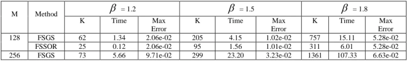
All numerical results for problems (9) and (10), obtained from application of FSGS and FSSOR iterative methods are recorded in Tables 1 and 2 by using the different value of mesh size, M=128, 256, 512, 1024 and 2048.

Table 1: Comparison of number iterations, the execution time ( seconds) and maximum errors for the iterative methods using example at 8

. 1 , 5 . 1 , 2 . 1  

M Method



= 1.2



= 1.5



= 1.8

K Time Max

Error

K Time Max

Error

K Time Max

Error

128 FSGS 62 1.34 2.06e-02 205 4.15 1.02e-02 757 15.11 5.28e-02

FSSOR 25 0.12 2.06e-02 95 1.56 1.01e-02 311 6.01 5.28e-02

256 FSGS 73 5.66 9.71e-02 299 23.20 3.23e-02 1361 107.33 6.63e-02

i.Initialize 10

~ 0and 10

U  

ii.For i=1,2,…,n-1 and j=1,2,…,m-1 assign

U 



D L



[ V (1 )D]U k



D L



1f ~

1 1

k ~

 

 _{ }

_

_

_{ }

_

_{ }

_

iii.Convergence test. If the convergence criterion i.e    k 10

~ 1 k

~ U 10

U   



  is satisfied, go step (iv)

FSSOR 30 2.22 9.71e-02 112 9.25 3.22e-02 432 49.23 6.63e-02

512 FSGS 84 26.18 1.79e-01 430 132.51 4.26e-02 2411 755.31 5.71e-02

FSSOR 34 9.21 1.79e-01 180 55.38 4.26e-02 941 226.24 5.71e-02

1024 FSGS 96 120.29 2.42e-01 613 755.97 4.82e-02 4221 5259.97 5.23e-02

FSSOR 42 60.08 2.42e-01 211 330.55 4.82e-02 1095 1201.30 5.23e-02

2048 FSGS 109 577.00 2.85e-01 866 4348.68 5.09e-02 7322 4979.18 5.09e-02

FSSOR 49 202.34 2.85e-01 396 1096.00 5.08e-02 2625 1121.10 5.09e-02

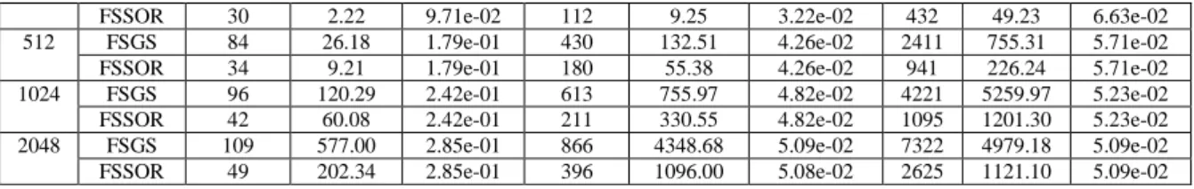
Table 2: Comparison of number iterations, the execution time ( seconds) and maximum errors for the iterative methods using example at 8

. 1 , 5 . 1 , 2 . 1  

M Method



= 1.2



= 1.5



= 1.8

K Time Max

Error

K Time Max

Error

K Time Max

Error

128 FSGS 48 1.19 1.82e-01 150 3.77 6.01e-02 473 11.36 6.31e-03

FSSOR 19 0.28 1.82e-01 85 1.23 6.01e-02 189 4.95 6.31e-03

256 FSGS 57 5.45 1.77e-01 225 21.61 7.64e-02 890 85.00 2.88e-02

FSSOR 23 2.01 1.77e-01 98 9.11 7.64e-02 394 39.25 2.88e-02

512 FSGS 67 25.31 1.52e-01 331 124.05 8.70e-02 1635 619.64 5.02e-02

FSSOR 27 9.15 1.52e-01 122 54.75 8.70e-02 461 212.10 5.02e-02

1024 FSGS 77 115.89 1.20e-01 477 714.51 9.00e-02 2937 4448.83 6.75e-02

FSSOR 33 52.00 1.20e-01 190 320.00 9.00e-02 983 1123.03 6.75e-02

2048 FSGS 88 557.00 1.04e-01 679 4259.31 9.25e-02 5171 55209.81 7.92e-02

FSSOR 39 198.22 1.04e-01 230 1232.00 9.25e-02 2126 19807.23 7.92e-02

Conclusion:

In this paper we proposed a Caputo’s implicit finite difference and scheme FSSOR method to solve the space-fractional diffusion equations. We have applied the formulation of the Caputo’s finite difference equations to generate a corresponding linear system. Then for solving the linear system, the formulation of FSGS and FSSOR iterative methods have been constructed based on the Caputo’s derivative operator. From observation of all experimental results by imposing the FSGS and FSSOR iterative methods, it can be also observed in tables 1 and 2 that the number of iterations and the execution time for FSSOR iterative method have been declined tremendously as compared with FSGS iterative method. This is due to the implementations of FSSOR iterative method have been accelerated by using the optimal value of the weighted parameter, ω. According to the accuracy and of both iterative methods, it can be concluded that their numerical solutions are in good agreement.

REFERENCES

Aslefallah, M. and D. Rostamy, 2014. A Numerical Scheme for Solving Space-Fractional Equation by Finite Difference Theta-Method. International Journal of Advances in Applied Mathematics and Mechanics, pp: 1-9.

Azizi, H. and G.B. Loghmani, 2013. Numerical Approximation for Space-Fractional Diffusion Equations via Chebyshev Finite Difference Method. Journal of Fractional and Applications, pp: 303-311.

Choi, H.W., S.K. Chung and Y.J. Lee, 2010. Numerical Solutions for Space-Fractional Dispersion Equations with Nonlinear Source Terms. Bull.Korean Math.Soc., pp: 1225-1234.

Evans, D.J., 1985. Group Explicit Iterative methods for solving large linear systems. International Journal Computer Maths, 17: 81-108.

Hackbusch, W., 1995. Iterative Solution of Large Sparse Systems of Equations. New York: Springer-Verlag.

Hadjidimos, A., 2000. Successive Over-relaxations and Relative Methods. Journal Of Computational and Applied Mathematics, 123: 177-199.

Othman, M. and A.R. Abdullah, 2000. An Efficient Four Points Modified Explicit Group Poisson Solver. International Journal Computer Mathematics, 76: 203-217.

Saad, Y., 1996. Iterative method for sparse linear systems. Boston: International Thomas Publishing. Saadatmandi, A. and M. Dehghan, 2011. A Tau Approach for Solution of The Space-Fractional Diffusion Equation. Journal of Computer and Mathematics with Applications, 62: 1135-1142.

Shen, S. and F. Liu, 2005. Error Analysis of an Explicit Finite Difference Approximation for The Space-Fractional Diffusion Equation with Insulated Ends. Journal ANZIAM, 46(E): C871-C878.

Starke, G. and W. Niethammer, 1991. SOR for AX – XB = C. Journal of Linear Algebra and Its Applications, 154: 355- 375.

Sun, Li-ying, 2005. A Comparison Theorem for The SOR Iterative Method. Journal of Computational and Applied Mathematics, 181: 336-341.

Young, D.M., 1954. Iterative Methods for Solving Partial Difference Equations of Elliptic Type. Trans. Amer. Math. Soc., 76: 92-111.

Young, D.M., 1971. Iterative Solution of large Linear Systems. London: Academic Press.

Young, D.M., 1972. Second-Degree Iterative Methods for The Solution of Large Linear Systems. Journal of Approximation Theory, 5: 37-148.

Yousif, W.S. and D.J. Evans, 1995. Explicit De-Coupled Group Iterative Methods and Their Implementations. Parallel Algorithms and Applications, 7: 53-71.

Youssef, I.K., 2012. On The Successive Over-relaxation Method. Journal of Mathematics and Statistics, 2: 176-184.