Stability Analysis of Conjunctivitis Model with Nonlinear Incidence Term

AENSI Journals

Australian Journal of Basic and Applied Sciences

ISSN:1991-8178

Journal home page: www.ajbasweb.com

Corresponding Author: Bundit Unyong, Department of Mathematics, Faculty of Science and Technology, Phuket Rajabhat University, Phuket, 83000, Thailand.

E-mail: [email protected], Ph: +66-804444435.

Stability Analysis of Conjunctivitis Model with Nonlinear Incidence Term

1_{BunditUnyong and}2_{Surapol Naowarat}

1_{Department of Mathematics, Faculty of Science and Technology, Phuket Rajabhat University, Phuket, 83000. Thailand.} 2_{Department of Mathematics, Faculty of Science and Technology, Suratthani Rajabhat University, SuratThani, 84100. Thailand.}

A R T I C L E I N F O A B S T R A C T Article history:

Received 30 September 2014 Received in revised form 17 November 2014 Accepted 25 November 2014 Available online 13 December 2014

Keywords:

Conjunctivitis, Nonliner incidence term, Stability, Equilibrium point, Basic reproductive number.

A simple SEIR model for Conjunctivitis is proposed and analyzed. In the present investigation of the dynamical and stability of Conjunctivitis model with nonlinear incidence term is taken into account. We used the incidence term as proportions of people that infected. The new incidence term 1

b

 

is used that shows the number of infected people in fraction. The standard method is used to analyze the behaviors of the proposed model. The results shown that there were two equilibrium points; disease free and endemic equilibrium point. The qualitative results are depended on a basic reproductive number(R )₀ . We obtained the basic reproductive number by using the next generation method and finding the spectral radius. Routh-Hurwitz criteria is used for determining the stabilities of the model. If R01, then the disease free equilibrium point is local asymptotically stable:

that is the disease will died out, but if R01, then the endemic equilibrium is local

asymptotically stable: that is the disease will also occur. The numerical results are shown for supporting the analytic results.

© 2014 AENSI Publisher All rights reserved. To Cite This Article: Bundit Unyong and Surapol Naowarat., Stability Analysis of Conjunctivitis Model with Nonlinear Incidence Term. Aust. J. Basic & Appl. Sci., 8(24): 52-58, 2014

INTRODUCTION

Conjunctivitis is an inflammation or infection of the conjunctiva. Sometime is called red eye or pink eye which the white eye has red more than usual or the eye has the red eye more than the other side. It may be caused by a viral or bacterial infection. It can also occur due to an allergic reaction to irritation the air like pollen and smoke, chlorine in swimming pools , and ingredients in cosmetics or other products that come in the contact with the eyes. In this papers, we are interested in Conjunctivitis caused by virus or know as Acute Hemorrhagic Conjunctivitis (AHC). It occurs in the eye that found frequently in Thailand especially during the rainy season because of the rain caused wetness and the virus is easily developed. Acute Hemorrhagic Conjunctivitis is simple and fast contact. This disease is caused by virus in Adenovirus group and Enterovirus group. Transmission occurs from person to person contract or contract with contaminated objects by tears of patients attached with fingers and transmit from finger to eye directly. The incubation period for each susceptible individual infect the virus is 1-2 days. The period of infection is about 14 days (Atchaneeyasakul, K. and V. Wiwanitkit, 2014; Bureau of Epidemiology, 1997-2011; Chowell, G., 2005).

R



1



bN





S I

E

I

S





E



I

(

 



)

I

E



R



model. They concluded that the rainfall is effect on the spread of this disease, to bring the epidemic under control more quickly, it is most important to educate the people in the community and correct prevention concept.

In this paper, we study the transmission of Acute Hemorrhagic Conjunctivitis through mathematical modeling. By used the standard method to analyze the behaviors of the proposed model.

2. Model Formulation:

To formulate our problem, we assumed that the human population is constant denoted by

N.

The human

population is divided into four compartments; the susceptible human

(S)



, the exposed human

( )

E



, the infected

human

(I)



and the recovered human

(R )



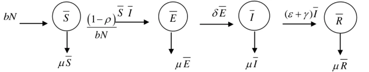
as shown in Fig. 1.

bN

Fig. 1: Flow chart of the dynamical transmission of Conjunctivitis.

We obtained the transmission model as shown by a system of ordinary differential equations as follows.

dS (1 )

bN S I S

dt bN

 

    (1)

dE (1 )

SI ( )E

dt bN

 

     (2)

d I

E ( ) I

dt         (3)

dR

( ) I R

dt       (4)

S   E I R N Where;

S(t)is the susceptible human population at time t E(t)is the exposed human population at time t I(t)is the infected human population at time t R(t)is the recovered human population at time t N is the total number of human population ,

b is the birth rate of human population ,  is the death rate of human population ,

 is the incubation rate of conjunctivitis in human population,  is the recovery rate of individuals who go to see the doctor ,

 is the recovery rate of individuals who don’t go to see the doctor,  is the fraction of individuals that to be infected.

The total size of population is assumed to be constant, therefore the rate of change for each human group equals to zero then the birth rate and the death rates are equivalent for the human populations that is b = μ .

We normalize equations (1)-(3) by letting S = S, E = E

N N and

I I =

N,then we get; The system of equations (5)-(7):

dS (1 )

b SI S

dt b

 

    (5)

dE (1 )

SI ( )E

dt b

 

     (6)

dI

E ( )I

dt        (7)

Where R(t) can be obtained from equation S(t)+E(t)+I(t)+R(t)=1

3. Analysis of the Model:

3.1 Basic properties of the model: The equilibrium points for * * *

(S ,E ,I ) are found by setting the right hand side of equation (5)-(7) equal to zero. We obtained two equilibrium points as follows;

b S

(1 )I b  _{ }

 

,E 1 b(1 ) I

( ) b (1 )I

   

 _{ }

   _     _ ,

b(1 ) b ( )( )

I

( )( )(1 )

             

         

3.1.1 Disease Free Equilibrium Point(E )₀ :

In the absence of the disease in the community, that is I=0, we obtained Sb, E0

 , then





0 0

b E S,E,I = E _ ,0,0_

  .

3.1.2 Endemic Equilibrium Point(E )1 :

In case the disease is presented in the community, I 0 , we obtained, * * * 1

E (S ,E ,I )where; *

* b S

(1 )I b 

  _{ }

* *

*

1 b(1 )

E I

( ) b (1 )I

   

 _{ }

   _     _

* b(1 ) b ( )( )

I

( )( )(1 )

             

         

3.2 Basic Reproductive Number(R )₀ :

We obtained a basic reproductive number by using the next generation method (van den Driessche and Watmough, 2002). By rewriting the equations (5) (7) in matrix form ;

dX F(X) V(X)

dt   (8)

Where F(X) is the non-negative matrix of new infection terms and V(X) is the non-singular matrix of remaining transfer terms.

Then we get;

(1 ρ)

0 b+ SI+μS

S _b

(1 ρ)

= E ,F(X)= SI ,V(X)= (δ+μ)E

b

I δE+(ε+γ+μ)I

0

dX

dt

  











_

_

 

_

_





 

_

_





 

_

_





 

 



_



_

_

_





(9)

And setting;

i 0

i

F (E )

F

X







 

_







and

i 0

i

V (E )

V

X







 

_







(10)

_{ρ FV}



1



_{. (11)} Where 1

FV is called the next generation matrix and _{ρ FV}



1



_{is the spectral radius of} 1 FV . For our model, the Jacobean matrix can be written as;

0

0 0 0

(1 )

F(E ) 0 0

0 0 0

   _{ }   _{ }      and ₀ (1 ) 0

V(E ) 0 ( ) 0

0 ( )

  _   _          _{     }       Hence, 2 2 1 0

1 (1 ) (1 )

( )( ) ( )

1

V (E ) 0 0

1 0 ( )( )          _{               }        _{  }                        1

0 0 0

(1 ) 1

FV 0

( )( ) ( )

0 0 0

    _{    }     _{ }                    Thus,

 



1



0 (1 ) FV E ( )( )               

Then we get the reproduction number

R

₀ where ,

0 (1 ) R ( )( )    

         (12) After some rearrangements * * *

1

E (S ,E ,I ) in term of R₀, we obtain;

* * 0

0 0

b b(R -1)

S = ,E =

μR (δ+μ)R and

* μb(R -1)0 I =

1-ρ .

3.3 Stability Analysis of the model:

In this section, we show the stability of both the disease-free equilibrium and endemic equilibrium point. First we have to show the system of equations (5)-(7) is locally asymptotically stable. To support this reason we use the disease-free equilibrium point E

0 about the system, the following Jacobean matrix J0 ,is presented.

Theorem 3.3.1:

ForR <1₀ , the disease-free equilibrium of the system of equations (5)-(7) ,about the equilibrium point E 0,is locally asymptotically stable and unstable whenever R >1₀ .

Proof:

To show the system of equations (5)-(7) is locally asymptotically stable ,we use the Jacobean matrix of the system of equations (5)-(7) evaluated at each equilibrium point. Then we get the following Jacobean matrix J₀,

0

(1 ) 0

1

J 0 ( )

0 ( )

   _   _        _     _                 (13)

0

(1 ) 0

1

J I 0 ( )

0 ( )

  

_{  } 

 _ 

 

 

 

  _       _



 

         

 

 

(14)

2 δ(1 ρ)

(λ+μ)[λ +(δ+2μ+ε+γ)λ+(δ+μ)(ε+γ+μ) ]=0 μ



 (15)

From the characteristic equation, we see that    ₁ 0,and the rest of the two eigenvalues are obtained by the Routh-Hurwitz criteria for stability. Next we have to show that,

a >0

and

b>0

for the pair of eigenvalues that we can get from equation (16) .

2 δ(1 ρ)

λ +(δ+2μ+ε+γ)λ+(δ+μ)(ε+γ+μ) =0 μ



 (16)

Where;

a=δ+2μ+ε+γandb=(δ+μ)(ε+γ+μ)-δ(1-ρ) μ .

Here

a

is clearly positive and for

b

with some arrangements, then we get,

0 b=(δ+μ)(ε+γ+μ)(1 R )>0

So that all eigenvalues associated to the system of equations (5)-(7) are having negative real parts. Thus we conclude that the system of equations (5)-(7) is locally asymptotically stable, when R <1.₀

3.4 Local Stability of Endemic Equilibrium:

In this section, we find the local asymptotic stability of the system of equations (5)-(7) about an endemic equilibrium pointE₁.

Theorem 3.2:

If R >1,₀ then the system of equations (5)-(7) about an endemic equilibrium point E₁is locally asymptotically stable, and unstable when, R <1₀ .

Proof:

For the system of equations (5)-(7),the Jacobean matrix J₁ ,is given by;

* *

* *

1

(1 ) I (1 )S

0

b b

(1 )I (1 )S

J ( )

b b

0 ( )

_{ }      

 

 

     

_     _

 

      

 

 

 

(17)

The eigenvalues of theJ₁ are obtained by solvingdet J



1 I3



0. Where;

* *

* *

1

(1 ) I (1 )S

0

b b

(1 )I (1 )S

J I ( )

b b

0 ( )

_{ }   _{ }    

 

 

     

  _       _

 

        

 

 

 

(18)

The characteristic equation of the above Jacobean matrix is

1 3

det(J λI )=0 (19)

3 2

1 2 3

λ +b λ +b λ+b =0

(20) Where;

1 0

b =ε+2μ+γ+δ+μR (21)

2 0 0 0

2

3 0

b =(μR ) (δ+μ)(ε+γ+μ)μδ(1 ρ) (23)

These eigenvalue are negative when the coefficients b ,b_{1 2} andb₃ are satisfy the Routh-Hurwitz criteria. 1) b >0₁

2) b >0₂

3) b b_{1 2}b >0₃

For the first condition we can see that b =ε+2μ+γ+δ+μR >0_{1 0} , then we consider the next conditions. We found thatb₂is positive when,

0 0 0

μR [(δ+μ+μR )(ε+γ+μ)+(μR )(δ+μ)]>δ(1 ρ)

And for the last condition ;b b b >0

1 2 3 . It is true when, 2

0

(μR ) (δ+μ)(ε+γ+μ)>μδ(1 ρ)

Then all three conditions satisfied the Routh-Hurwitz condition. We deduce that

1

E is local asymptotically stable when R >1.₀

IV.Numerical Results:

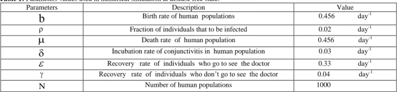
The parameters used in the numerical simulation are given in Table 1.

Table 1: Parameters values used in numerical simulation at disease free state.

Parameters Description Value

b

Birth rate of human populations 0.456 day-1

 Fraction of individuals that to be infected 0.02 day-1



Death rate of human population 0.456 day-1



Incubation rate of conjunctivitis in human population 0.03 day-1



Recovery rate of individuals who go to see the doctor 0.33 day-1  Recovery rate of individuals who don’t go to see the doctor 0.04 day-1

N Number of human populations 1000

Stability of disease free state:

From the values of parameters in Table 1 , we obtained the eigenvalues and basic reproductive number are :

10.456, 20.962, 30.350

   ,  ₀ 0.1625751.

Since all of eigenvalues are to be negative and the basic reproductive number is to be less than one, the disease free equilibrium (E₀) will be local asymptotically stable ,as shown in Fig. 2.

(a) (b) (c)

Fig. 2: Time series of (a) Susceptible human

(S)

; (b) Exposed human

(E)

; (c) Infected human

(I)

.The value of parameters are in the text and R01. We see that the solutions converge to the disease free

stateE 1,0,00





as shown.

Stability of endemic state:

We change the value of the fraction of individuals that to be infected ; 0.002,the incubation rate of

1 0.456, 2 1.737, 3 0.089

      ,  ₀ 1.1261 1 .

Since all of eigenvalues are to be negative and the basic reproductive number is to be greater than one, the endemic equilibrium (E )₁ will be local asymptotically stable as seen in Fig. 3

(a) (b) (c)

Fig. 3: Time series of (a) Susceptible human

(S)

; (b) Exposed human

(E)

; (c) Infected human

(I)

. The values of parameters are in the text andR01. We see that the solutions converge to the endemic

stateE 0.57,₁



0.25, 0.16



as shown.

V. Discussion and Conclusion:

From the model, we have calculated the basic reproductive number through the use of spectral radius of the

next generation matrix. The basic reproductive number is 0 R0 ,where 0

(1 ) R

( )( )

   

         . The basic reproductive number is the threshold condition for investigating the stability of the solutions of model as shown in Fig. 2 and 3. Our simulated results showed that ₀will increase when the fraction of individuals that to be

infected

( )



decrease, We found that the values of R₀were 0.1625758, 1.1260740. when 0.02, 0.002, respectively. It seen that if the infected human increase then the fraction of individuals that to be infected is decreased.

ACKNOWLEDGEMENT

The authors are grateful to the Department of Mathematics, Faculty of Science and Technology, Phuket Rajabhat University, Thailand for providing the facilities to carry out the research.

REFERENCES

Atchaneeyasakul, K. and V. Wiwanitkit, 2014. Overview of Conjunctivitis in Thailand. Update In Infected Disease, 21-24.

Bureau of Epidemiology, 1997-2011. Acute Hemorrhagic Conjunctivitis [online] Available: at: http://www.boe.moph.go.th.

Chowell, G., E. Shim, F. Brauer, P. Diaz-Dueňas, J.M. Hyman1 and C. Castillo - Chavez,2005. “Modelling the transmission dynamics of acute haemorrhagic conjunctivitis: Application to the 2003 outbreak in Mexico.” Wiley Online Library [On-line serial]. Available: DOI: 10.1002/sim.2352.

Chulalongkornhospital, 2012. viral conjunctivitis. [online] Available at: http://www.chulalongkornhospital.go.th.

Ghazali, O., K.B. Chua, K.P. Ng, P.S. Hooi, M.A. Pallansch, M.S. Oberste, K.H. Chua, J.W. Mak, 2003. An Outbreak of Acute Haemorrhagic Conjunctivitis in Melaka, Malaysia. Singapore Medical Journal, 44(10): 511-516.

Kunawisarut, S., 2012. hemorrhagic conjunctivitis. [online] Available at: http://haamor.com/knowledge. Sangsawang, S., T. Tanutpanit, W. Mungtong and P. Pongsumpun, 2012. Local Stability Analysis of Mathematical Model for Hemorrhagic Conjunctivitis Disease. KMITL. Sci. Tech. J., 12(2): 189-197.

Jantraporn Suksawat and Surapol Naowarat,(2014.) Effect of Rainfall on the Transmission Model of Conjunctivitis. Adv. Environ. Biol., 8(14), 99-104, 2014