1. Classical to quantum mechanical transition
Classical mechanics, based on Newton’s laws of motion, successfully describes the motion of all macroscopic objects such as a falling stone, orbiting planets etc., which have essentially a particle-like behaviour. However it fails when applied to microscopic objects like electrons, atoms, molecules etc. This is mainly because of the fact that classical mechanics ignores the concept of dual behaviour of matter especially for sub-atomic particles and the uncertainty principle. The branch of science that takes into account this dual behaviour of matter is called quantum mechanics.
Quantum mechanics is a theoretical science that deals with the study of the motions of the microscopic objects that have both observable wave like and particle like properties. It specifies the laws of motion that these objects obey. When quantum mechanics is applied to macroscopic objects (for which wave like properties are insignificant) the results are the same as those from the classical mechanics.
Quantum mechanics was developed independently in 1926 by Werner Heisenberg and Erwin Schrödinger. Here, however, we shall be discussing the quantum mechanics which is based on the ideas of wave motion. The fundamental equation of quantum mechanics was developed by Schrödinger and he won Nobel Prize in Physics in 1933.
2. Electromagnetic radiation
2.1. Wave nature of Electromagnetic Radiation
For the first time in 1870 James Maxwell explained comprehensively about the interaction between the charged bodies and the behaviour of electrical and magnetic fields on macroscopic level. He suggested that when electrically charged particle moves under acceleration, alternating electrical and magnetic fields are produced and transmitted. These fields are transmitted in the forms of waves called electromagnetic waves or electromagnetic radiation.
Light is the form of radiation known from early days and in earlier days (Newton) light was thought to be made of particles (corpuscules). It was only in the 19th century when wave nature of light was established. Maxwell was again the first to reveal that light waves are associated with oscillating electric and magnetic character.
2.2. Particle nature of Electromagnetic Radiation – Planck concept
Some of the experimental phenomenon such as diffraction (is the bending of wave around an obstacle) and interference (is the combination of two waves of the same or different frequencies to give a wave whose distribution at each point in space is the algebraic or vector sum of disturbances at that point resulting from each interfering wave.) can be explained by the wave nature of the electromagnetic radiation. However, following are some of the observations which could not be explained with the help of even the electromagnetic theory of 19th century physics (known as classical physics):
The nature of emission of radiation from hot bodies (black -body radiation)
Ejection of electrons from metal surface when radiation strikes it (photoelectric effect) Variation of heat capacity of solids as a function of temperature
Line spectra of atoms with special reference to hydrogen.
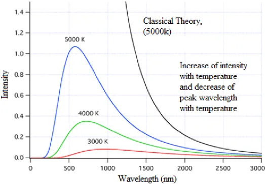
When solids are heated they emit radiation over a wide range of wavelengths. For example, when an iron rod is heated, it first turns to dull red and then progressively becomes bright red with temperature rise. Further heating, the radiation emitted becomes white and then becomes blue as the temperature becomes very high. In terms of frequency, it means that the frequency of emitted radiation goes from a lower frequency to a higher frequency as the temperature increases. The red colour lies in the lower frequency region while blue colour belongs to the higher frequency region of the electromagnetic spectrum. “An ideal body, which emits and absorbs radiations of all frequencies, is called a black body and the radiation emitted by such a body is called black body radiation”.
The exact frequency distribution of the emitted radiation (intensity versus frequency curve) from a black body depends only on its temperature. At a given temperature, intensity of radiation emitted increases with decrease of wavelength, reaches a maximum value at a given wavelength and then starts decreasing with further decrease of wavelength, and is shown in the below Fig: 1
Fig: 1 intensity versus frequency curve
The above experimental results cannot be explained satisfactorily on the basis of the wave theory of light. Planck suggested that atoms and molecules could emit (or absorb) energy only in discrete quantities and not in a continuous manner, a belief popular at that time. Planck gave the name quantum to the smallest quantity of energy that can be emitted or absorbed in the form of electromagnetic radiation. The energy (E) of a quantum of radiation is proportional to its frequency (ν) and is expressed by the Equation: 1;
E = hν (1)
With this theory, Planck was able to explain the distribution of intensity in the radiation from black body as a function of frequency or wavelength at different temperatures.
3. Origin of quantum mechanics: Attempts were made to develop a more suitable and general model for atoms, in order to overcome shortcoming of the Bohr’s model. In this connection, two important developments which contributed significantly in the formulation of such a model were:
3.1. Dual behaviour of matter
3.2. Heisenberg uncertainty principle
3.1. Dual nature of light and matter
The French physicist, de Broglie in 1924 proposed that matter, like radiation, should also exhibit dual behaviour i.e., both particle and wavelike properties. This means that just as the photon has momentum as well as wavelength, electrons should also have momentum as well as wavelength, de Broglie, from this analogy, gave the following Equation: 2, between wavelength (λ) and momentum (p) of a material particle.
λ = h / mv = h / p (2)
Where; m is the mass of the particle, v its velocity and p its momentum.
Derivation: The de Broglie equation can be easily derived with the help of mass-energy relationship. E=���, and energy of photon E = hν.
Therefore we have from E=��� andE = hν,
���= hν (3)
But, c = νλ and therefore ν = c / λ
Substituting for ν in equation (3) we have, ���= h (c / λ) (4)
Rearranging the equation (4), we have finally λ = h / mv, hence the equation (2).
3.2. Heisenberg uncertainty principle
According to classical mechanics a moving particle has a definite momentum and occupies a definite position in space and it is possible to determine both its position and momentum. But it has been seen that classical point of view represents an approximation which is adequate for the objects of appreciable site, but does not describe satisfactorily the behavior of the particles of atomic dimensions. In other words we can say classical concept does not hold in the region of atomic dimensions.
Mathematically if x and p are the uncertainties in the position and momentum of a particle,
then
Δx
.
Δp
≥
h
4
π
(5)The constancy of the product of uncertainties means that the two are inversely proportional to each other. Thus if the position of an electron is known with certainty, then its momentum cannot be known and vice-versa.
3.2.1. Physical significance of Heisenberg’s uncertainty principle
a. One of the important implications of the Heisenberg Uncertainty Principle is that it rules out existence of definite paths or trajectories of electrons and other similar particles.
b. Nonexistence of electrons inside the nucleus: If an electron can exist inside the nucleus, it must have a minimum energy of about 20 MeV. But beta (ß) decay studies indicate that the kinetic energy of β-particle emission from nucleus is found to be of the order of 3 to 4 MeV. Hence, we can conclude that electron cannot exist inside the nucleus.
3.3. Einstein concept of photoelectric theory
Classical physics predicted that the number of electrons emitted from a metal surface and their kinetic energy should depend on only the intensity of the light, not its frequency.
Albert Einstein used realised Planck’s hypothesis about the quantization of radiant energy could also explain the photoelectric effect. The key feature of Einstein’s hypothesis was the assumption that radiant energy arrives at the metal surface in particles which are known as photons, a quantum of radiant energy, each of which possesses a particular energy given by E=hν. Einstein postulated that each metal has a particular electrostatic attraction for its electrons that must be overcome before an electron can be emitted from its surface (Eo = hνo). If photons of light with
energy less than Eo strike a metal surface, no single photon has enough energy to eject an
electron, so no electrons are emitted regardless of the intensity of the light. If a photon with energy greater than Eo strikes the metal, then part of its energy is used by electron to overcome
the forces that hold the electron to the metal surface, and the excess energy appears as the kinetic energy of the ejected electron, as mentioned in Equation: 6.
Kinetic energy of ejected electron = E − Eo = hν − hνo = h (ν − νo) (6)
When a metal is struck by light with energy above the threshold energy Eo, the number of emitted
electrons is proportional to the intensity of the light beam, which corresponds to the number of photons per square centimeter, but the kinetic energy of the emitted electrons is proportional to the frequency of the light. Thus Einstein showed that the energy of the emitted electrons depended on the frequency of the light, contrary to the prediction of classical physics
4. Schrödinger wave equation and wave functions, particle in a box (1D)
4.1. Wave function (Ψ)
The quantity that gives all possible information about a particle that exhibits wave-character is called a wave function. Wave function gives complete information about the state of a physical system at a particular time.
4.2. Physical significance of wave function
The wave function is a solution of Schrodinger wave equation.
The wave function gives the probability of finding a particle at a particular position. The wave function is a complex quantity where as its probability must be real and
positive.
The wave function cannot be measured directly by any physical experiment. However the knowledge of useful dynamical variables such as position, momentum, Kinetic energy, Potential energy etc. of the particle are obtained by performing suitable mathematical operations on the wave function.
It is large in magnitude where the particles such as electrons or protons are likely to be
located and small at other places.
4.3. Probability density (P)
The probability of finding a particle is described by the wave function ψ at the point (x, y, z)
at the time instant t is proportional to
|
ψ
|
2 i.e. the square of the amplitude of the wave functionat that instant. To be more specific, if ψ represents a single particle, then
|
ψ
|
2 is called the probability density. It is the probability per unit volume that the particle will be found within an infinitesimal volume containing the point x.4.4. Eigen values and Eigen functions
4.4.1. Eigen functions: As we know Schrodinger equation is a second order differential equation. There is no one solution but many solutions of the equation. All the solutions, which can express in terms of wave functions, may not be the correct wave functions, which we are searching for. We have to select those wave functions, which would correspond meaningfully to a physical system. Such wave functions are said to be acceptable wave function or Eigen function.
4.4.2. Eigen values: Eigen functions when operated with quantum mechanical operators (energy or momentum), leads to physical observables such as energy, momentum of the particle. Such values are called as Eigen values.
4.5. The Schrödinger Time independent wave equation
Schrödinger equation is the fundamental equation of quantum mechanics. It is a wave equation capable of determining the wave function ψ of the matter waves in different physical situations. The Schrodinger equation can be set up for both time dependent and time independent states.
4.5.1. Time independent Schrodinger wave equation
Schrodinger wave equation. Consider a one –dimensional wave function ψ for a particle moving freely in the positive x- direction.
The wave function is specified by; (1)
Where; ‘A’ is the amplitude of the wave, ω is angular frequency, and K is wave number. Equation (1) describes the wave equivalent of an unrestricted particle of total energy E and momentum P in the x-direction. Differentiating equation (1) with respect to t we get,
dΨ
dt =−ωA e
i(Kx−ωt)
d
2 Ψ d t2 =−ω
2
[
A ei(Kx−ωt)
]
d2Ψ d t2 =−ω
2Ψ
(2)
The equation for travelling wave is
d2y d x2=
1
v2 d2y
d t2
(3)
Where; y is the displacement, v is velocity of the wave. By the analogy, wave equation for de-Broglie wave is;
d2Ψ d x2=
1
v2 d2Ψ
d t2
By substituting equation (2)
d
2Ψ
d x2=
−ω2Ψ v2
If λ and ν are the wavelength and frequency of the wave then λ=2πγ and v=γ λ
d
2 Ψ d x2=
−4π2Ψ λ2
1
λ2=
−1 4π2Ψ
d2Ψ
d x2 - (4)
For a particle of mass m moving with a velocity v,
K . E=1 2m v
2
= P
2
2m
De-Broglie equation is p=h/λ
K . E= h
2
2m
1
λ2 (6)
Substituting (3) in (5)
K . E= h
2
2m
−1 4π2Ψ
d2Ψ d x2
(7)
If the total energy of the particle is E, then E= K.E +V
Where; V is potential energy.
K.E = (E-V) Substituting in equation (7),
(E−V)= h
2
2m
−1 4π2Ψ
d2Ψ d x2
d2Ψ d x2=
−8m π2
h2 (E−V)Ψ
d2Ψ d x2 +
8mπ2
h2 (E−V)Ψ=0
(8)
This equation is known as Schrodinger time independent wave equation in one dimension.
For a free particle V=0 d
2 Ψ d x2 +
8mπ2
h2 (E)Ψ=0
Extending the equation to 3- dimensions, the Schrödinger time independent equation will be,
d2Ψ d x2 +
d2Ψ d y2+
d2Ψ d z2+
8m π2
h2 (E−V)Ψ=0 (9)
∇2
Ψ+8m π
2
h2 (E−V)Ψ=0
Where;
∇
2= ∂
2∂
x
2+ ∂
2
∂
y
2+ ∂
2
∂
z
2 is called de-Alembert’s operator.Note: From equation (8)
d2Ψ d x2 +
8mπ2
d2Ψ d x2 +
8mπ2
h2 (K . E)Ψ=0
d2Ψ d x2=
−8m π2
h2 (K . E)Ψ
−h2
8m π2 d2Ψ
d x2=(K . E)Ψ
(
−h28m π2 d2
d x2
)
Ψ=(K . E)ΨHence;
(
−h2
8m π2 d2
d x2
)
=Energy operator.4.6. Applications of Schrodinger wave equation
4.6.1. Particle in one-dimensional potential well (box) of infinite height
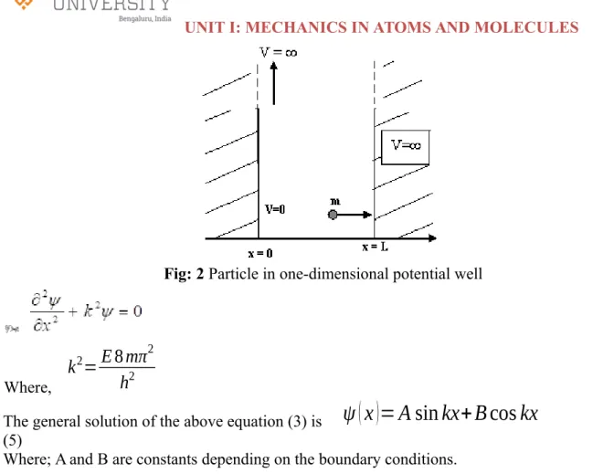
Consider a particle of mass ‘m’ moving inside a box along the X – direction between two rigid walls A and B. The particle is free to move between the walls of the box at x = 0 and x = L. The potential energy of the particle is considered to be zero inside the box and infinity at all points outside the box. This means that;
(i) PE, V= 0 for 0<x< L
(ii) PE, V=∞ for x ≤ 0 and x ≥ L
The particle moves freely in the region between x=0 and x=L. As the particle recoils elastically it does not lose energy when it collides with walls, so its energy remains constant. Since the particle is a free particle, its potential energy is zero. The particle cannot have an infinite amount of energy. Itcannot exist outside the box, so its wave function and is shown in Fig: 2
The Schrodinger wave equation is given by d
2 Ψ d x2 +
8mπ2
h2 (E−V)Ψ=0 (1)
Since inside the box, potential energy, V=0 d
2Ψ
d x2 +
8mπ2
Fig: 2 Particle in one-dimensional potential well
(3)
Where,
k
2=
E
8
mπ
2h
2 (4)The general solution of the above equation (3) is
ψ
(
x
)
=
A
sin
kx
+
B
cos
kx
(5)Where; A and B are constants depending on the boundary conditions.
Case-1
ψ
=
0
atx
=
0
Then equation (4) becomes
B
=
0
(6)Case-2
ψ
=
0
at x=L
0
=
A
sin
kL
+
B
cos
KL
Since B=0 AsinKL=0
sin
kL
=
0
=
sin
nπ
⇒
kL
=
nπ
⇒
k
=
nπ
L
(7)Where n= 0, 1, 2, 3…
Substituting the value of
B
=
0
and k=nπ
L in equation (5) we get.
(8)
Which represents the permitted solutions from equation (3)
Substituting k=
nπ
(10)
The above equation gives the allowed values of energy for different values of n. The possible values of the energy are called Eigen values and the corresponding values of ψ are called Eigen functions.
The Eigen values are
E
1=
h
28
mL
2, E
2=
4
h
28
mL
2, E
3=
9
h
28
mL
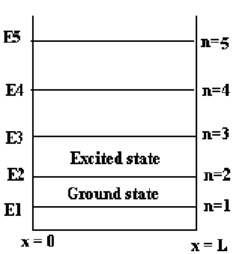
2 and so on.The energy corresponding to n=1 is called ground state energy or Zero-point energy and the other energies are called excited states energy.
E
0=
h
28
mL
2 , is called Zero point energy.For each value of n, there is an energy level. The possible allowed values of energy obtained from Equation: 10 i.e. E1, E2, E3 etc. are called Eigen values and the corresponding wave function ψn is called the Eigen function. The following Fig: 3 depictsthe occupation of various
energy levels occupied by particle.
Fig: 3 Particle energy levels for a given quantum number
The energy corresponding to n = 1 is called ground state energy or zero point energy. And energy levels for n = 2,3,4,5, etc. are called excited states. Inside the well, the particles can have discrete set of values of energy and it is quantized. E2 = 4E0, E3 = 9E0, E4 = 16E0, and so on.
Evaluation of A
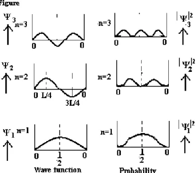
(11) The corresponding normalized wave function of a particle in a one dimensional box is given by the Equation: 12.
(12) The normalization wave functions Ψ1, ψ2, ψ3 are together with the probability densities
|
ψ
1|
2,
|
ψ
2|
2,
|
ψ
3|
2 are plotted as shown in Fig: 4.Although ψn may be negative as well as positive, but
|
ψ
n|
2
is always positive. Fig: 4 indicates the probability of finding the particle at different locations inside the box. In every case,
|
ψ
n|
2=
0
at x=0 and x=L which are the boundaries conditions for a particle in 1Dbox.
Note: The value of, A=
√
(
2L
)
is called as normalization constant.5. Classical and quantum mechanics – Distinction
Classical Mechanics Quantum Mechanics Deals with macroscopic bodies Deals with microscopic particles
Based on Newton’s laws of motion Both Heisenberg’s uncertainty principle and de-Broglie concept of particle dual nature, guide quantum mechanics
Amount of energy emitted or absorbed by matter is continuous and is based on Maxwell’s electromagnetic theory.
Absorption or emission of energy is discontinuous and is based on Planck’s quantum theory.
Both position and momentum of a particle certain, both can be determined simultaneously.
Both position and momentum of a particle uncertain, and both cannot be determined simultaneously. That is, quantum mechanics tells probability of finding a particle in space.
6. Quantum numbers
In an atom number of orbitals vary based on its atomic number. Qualitatively these orbitals can be distinguished by their size, shape and orientation. In an orbital of smaller size, there is more chance of finding the electron near the nucleus. Also, the shape and orientation of the orbital indicates probability of finding the electron more along certain directions than along others. Atomic orbitals are precisely distinguished by what are known as quantum numbers. Each orbital is designated by three quantum numbers labelled as n, l and ml. The fourth one is the spin
quantum number s of electron, which will be + ½ or – ½.
6.1. Principal quantum number (‘n’): It is a positive integer with value of n = 1, 2, 3 etc. It determines the size and energy of the orbital. Further, the principal quantum number also represents the shell. With the increase in the value of ‘n’, the number of allowed orbital increases and are given by ‘n2’. All the orbitals of a given value of ‘n’ constitute a single shell of atom and
are represented by the following letters;
n = 1, 2, 3, 4, ---
Shell = K, L, M, N,
---6.2. Azimuthal quantum number (l). It is denoted by ‘l’ and is also known as orbital angular momentum or subsidiary quantum number. The value of ‘l’ denotes three dimensional shape of the orbital. For a given value of n, l can have n values ranging from 0 to n – 1, that is, for a given value of n, the possible value of ‘l’ are: l = 0, 1, 2, ... (n–1).
For example;
For n = 1, ‘l’ can have only 0. For n = 2, ‘l’ can have only 0 and 1.
6.3. Magnetic orbital quantum number (‘ml’): The ‘ml’ value gives information about the
spatial orientation of the orbitals. For any sub-shell (defined by ‘l’ value), 2l+1 values of ml are
possible and are given by: ml = – l, – (l–1), – (l–2)... 0, 1... (l –2), (l–1), l
For example:
For l = 0, ml = 0, [2(0) +1] = 1, one ‘s’ orbital.
For l = 1, ml = –1, 0 and +1 [2(1) +1] = 3, three ‘p’ orbitals.
For l = 2, ml = –2, –1, 0, +1 and +2, [2(2) +1] = 5, five ‘d’ orbitals.
6.4. Spin quantum number (ms): An electron spins around its own axis. This means, an
electron possess intrinsic spin angular quantum number, besides charge and mass. Spin angular momentum of the electron is a vector quantity, and can have two orientations relative to the chosen axis. These two orientations are distinguished by the spin quantum numbers ms, whose
values can be either +½ or –½. These are also represented by two arrows, ↑ (spin up) and ↓ (spin down), respectively.
7. Orbital degeneracy
Orbital degeneracy means, two or more different states of a quantum mechanical system are said to be degenerate if they give the same value of energy upon measurement. The number of different states corresponding to a particular energy level is known as the degree of degeneracy of the level. For both d and p orbitals, the degeneracy can be depicted as shown in the following Fig: 5
Fig: 5 - Degenerate states in a quantum system
In a quantum mechanical system the degeneracy may be removed by an external perturbation or disturbance. As a consequence, splitting in the degenerate energy levels occurs. Mathematically, the splitting due to the application of a small perturbation potential can be calculated using time-independent degenerate perturbation theory.
The splitting of the energy levels of an atom when placed in an external magnetic field because of the interaction of the magnetic moment of the atom with the applied field is known as the Zeeman Effect.
7.2. Stark effect
The splitting of the energy levels of an atom or molecule when subjected to an external electric field is known as the Stark effect.
8. Magnetic behaviour of matter
Matter is composed of atoms consisting of positively charged nuclei and negative electrons. These electrons present in shells, and the periodic nature of chemical properties of atoms as the atomic weight increases is a reflection of the fact that the chemical behavior of an atom depends largely upon the number of electrons in the outermost shell.
The magnetic properties of matter arise from two sources. An electron in orbital motion about the nucleus constitutes a small circulating current, which generates a magnetic field. The electron moving in its orbit has an angular momentum about the nucleus. In addition to the magnetism due to its orbital motion, an electron has an intrinsic magnetic moment and an intrinsic angular momentum, owing to its spin. In the absence of a magnetic field, the orbital magnetic moments and the intrinsic magnetic moments of different electrons are randomly oriented within matter. Most materials are only very slightly magnetic in the presence of external magnetic fields. They are said to be either diamagnetic or paramagnetic. A diamagnetic material is one for which Km is
less than 1. The magnetic effects induced in the material are opposed to the external field. We would expect materials to be diamagnetic if the orbital electronic effects predominated, for, in accordance with Lenz's law, the magnetic effects induced in a circuit must be in such a direction as to oppose the change in magnetic field in the substance. A paramagnetic material is one for which Km is greater than 1. A paramagnetic substance will experience a force in the opposite
direction. In general, in all materials except those called ferromagnetic (that is, those which behave like iron), the magnetic effects are quite small, and these materials may be treated as though their relative permeability Km is 1, to an accuracy of about 0.1 per cent. A ferromagnetic
substance is attracted into a magnetic field with a large force. The relative permeability Km of a
ferromagnetic substance may be as large as 104 or 105. Ferromagnetic substances are therefore
special cases of the general class of paramagnetic substances. The subject of ferromagnetism is of great importance in electrical engineering, and is as complex as it is important. The properties of ferromagnetic substances form the basis of the practical design of motors, generators, transformers, magnetic amplifiers, tape recorders, loud-speakers, permanent magnets, and a host of other devices.
9. Wave functions in bonding in molecules (H2)
In the classic case of covalent bonding, the H2 molecule forms by the overlap of the wave
functions of the electrons of the respective hydrogen atoms in an interaction which is characterized as an exchange interaction. When overlap creates an increase in electron density in the region between the two nuclei a sigma bond (σ bond) is formed. The same has been depicted in Fig-6.
The wave function
ᴪ
for the H2 molecule can be described in terms of the atomic wavefunctions
ᴪ
H1 andᴪ
H2 as follows;=
ᴪ ᴪ
H1ᴪ
H2(13)
For convenience purposes we will explicitly include the location of the valence electron for each atomic wave function;
ᴪ
=ᴪ
H1 (1s1H1)ᴪ
H2 (1s1H2) (14)As both H atoms approach each other and orbital overlap occurs, electrons 1s1
H1 and 1s1H2
become indistinguishable from each other, thus an equally valid representation of
ᴪ
is;ᴪ
=ᴪ
H1 (1s1H2)ᴪ
H2 (1s1H1) (15)As such, when the interatomic distance of both H atoms is within the bonding regime, the true state of the system is more accurately described as a linear combination of both of the probable wave functions;
ᴪ
= N [ᴪ
H1 (1s1H1)ᴪ
H2 (1s1H2) ±ᴪ
H1 (1s1H2)ᴪ
H2 (1s1H1)] (16)The two possibilities for the radial wave functions of distant hydrogens are shown below.
The symmetric wave function represented by
ᴪ
S interferes constructively (+) resulting in anenhancement in the value of the wave function in the internuclear region, resulting σ bonding orbital is the result. The anti symmetric wave function represented by ‐
ᴪ
A interferes destructively(-) resulting in decrease in the value of the wave function in the internuclear region, resulting σ*
antibonding orbital.
(a) σ Bonding;
ᴪ
= N [ᴪ
H1 (1s1H1)ᴪ
H2 (1s1H2) +ᴪ
H1 (1s1H2)ᴪ
H2 (1s1H1)](b) σ*Antibonding;
ᴪ
= N [ᴪ
H1 (1s1H1)
ᴪ
H2 (1s1H2) -ᴪ
H1 (1s1H2)ᴪ
H2 (1s1H1)]9.0. Periodic properties of elements
The elements in the periodic table are arranged in order of increasing atomic number. All of these elements display several other trends and we can use the periodic law and table formation to predict their chemical, physical, and atomic properties. Understanding these trends is done by analyzing the elements electron configuration; all elements prefer an octet formation and will gain or lose electrons to form that stable configuration. These trends explain the periodicity observed in the elemental properties of atomic radius, ionization energy, electron affinity, and electronegativity.
9.1. Atomic Radius
The atomic radius of an element is half of the distance between the centers of two atoms of that element that are just touching each other. Generally, the atomic radius decreases across a period from left to right and increases down a given group. The atoms with the largest atomic radii are located in Group I and at the bottom of groups.
Moving from left to right across a period, electrons are added one at a time to the outer energy shell. Electrons within a shell cannot shield each other from the attraction to protons. Since the number of protons is also increasing, the effective nuclear charge increases across a period. This causes the atomic radius to decrease.
Moving down a group in the periodic table, the number of electrons and filled electron shells increases, but the number of valence electrons remains the same. The outermost electrons in a group are exposed to the same effective nuclear charge, but electrons are found farther from the nucleus as the number of filled energy shells increases. Therefore, the atomic radii increase.
9.2. Ionization Energy
second ionization energy is always greater than the first ionization energy. Ionization energies increase moving from left to right across a period (decreasing atomic radius). Ionization energy decreases moving down a group (increasing atomic radius). Group I elements have low ionization energies because the loss of an electron forms a stable octet.
9.3. Electron Affinity
Electron affinity reflects the ability of an atom to accept an electron. It is the energy change that occurs when an electron is added to a gaseous atom. Atoms with stronger effective nuclear charge have greater electron affinity. Some generalizations can be made about the electron affinities of certain groups in the periodic table. The Group IIA elements, the alkaline earths, have low electron affinity values. These elements are relatively stable because they have filled s subshells. Group VIIA elements, the halogens, have high electron affinities because the addition of an electron to an atom results in a completely filled shell. Group VIII elements, noble gases, have electron affinities near zero since each atom possesses a stable octet and will not accept an electron readily. Elements of other groups have low electron affinities.
In a period, the halogen will have the highest electron affinity, while the noble gas will have the lowest electron affinity. Electron affinity decreases moving down a group because a new electron would be further from the nucleus of a large atom.
9.4. Electronegativity
Electronegativity is a measure of the attraction of an atom for the electrons in a chemical bond. The higher the electronegativity of an atom, the greater its attraction for bonding electrons. Electronegativity is related to ionization energy. Electrons with low ionization energies have low electronegativities because their nuclei do not exert a strong attractive force on electrons. Elements with high ionization energies have high electronegativities due to the strong pull exerted on electrons by the nucleus. In a group, the electronegativity decreases as the atomic number increases, as a result of the increased distance between the valence electron and nucleus (greater atomic radius). An example of an electropositive (i.e., low electronegativity) element is cesium; an example of a highly electronegative element is fluorine.
Summary of Periodic Properties of Elements
Left → Right (across the period) Atomic Radius Decreases Ionization Energy Increases
Electron Affinity Generally Increases (except Noble gas electron affinity near zero) Electronegativity Increases
Top → Bottom (Down the group) Atomic Radius Increases Ionization Energy Decreases