Recommendation Systems
There is an extensive class of Web applications that involve predicting user responses to options. Such a facility is called a recommendation system. We shall begin this chapter with a survey of the most important examples of these systems. However, to bring the problem into focus, two good examples of recommendation systems are:1. Offering news articles to on-line newspaper readers, based on a prediction of reader interests.
2. Offering customers of an on-line retailer suggestions about what they might like to buy, based on their past history of purchases and/or product searches.
Recommendation systems use a number of different technologies. We can classify these systems into two broad groups.
• Content-based systemsexamine properties of the items recommended. For instance, if a Netflix user has watched many cowboy movies, then recom-mend a movie classified in the database as having the “cowboy” genre. • Collaborative filteringsystems recommend items based on similarity
mea-sures between users and/or items. The items recommended to a user are those preferred by similar users. This sort of recommendation system can use the groundwork laid in Chapter 3 on similarity search and Chapter 7 on clustering. However, these technologies by themselves are not suffi-cient, and there are some new algorithms that have proven effective for recommendation systems.
9.1
A Model for Recommendation Systems
In this section we introduce a model for recommendation systems, based on a utility matrix of preferences. We introduce the concept of a “long-tail,”
which explains the advantage of on-line vendors over conventional, brick-and-mortar vendors. We then briefly survey the sorts of applications in which recommendation systems have proved useful.
9.1.1
The Utility Matrix
In a recommendation-system application there are two classes of entities, which we shall refer to asusersanditems. Users have preferences for certain items, and these preferences must be teased out of the data. The data itself is repre-sented as autility matrix, giving for each user-item pair, a value that represents what is known about the degree of preference of that user for that item. Values come from an ordered set, e.g., integers 1–5 representing the number of stars that the user gave as a rating for that item. We assume that the matrix is sparse, meaning that most entries are “unknown.” An unknown rating implies that we have no explicit information about the user’s preference for the item.
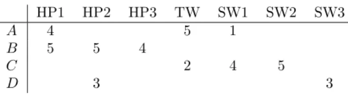
Example 9.1 : In Fig. 9.1 we see an example utility matrix, representing users’ ratings of movies on a 1–5 scale, with 5 the highest rating. Blanks represent the situation where the user has not rated the movie. The movie names are HP1, HP2, and HP3 forHarry PotterI, II, and III, TW forTwilight, and SW1, SW2, and SW3 for Star Warsepisodes 1, 2, and 3. The users are represented by capital letters AthroughD.
HP1 HP2 HP3 TW SW1 SW2 SW3
A 4 5 1
B 5 5 4
C 2 4 5
D 3 3
Figure 9.1: A utility matrix representing ratings of movies on a 1–5 scale Notice that most user-movie pairs have blanks, meaning the user has not rated the movie. In practice, the matrix would be even sparser, with the typical user rating only a tiny fraction of all available movies. 2
The goal of a recommendation system is to predict the blanks in the utility matrix. For example, would user A like SW2? There is little evidence from the tiny matrix in Fig. 9.1. We might design our recommendation system to take into account properties of movies, such as their producer, director, stars, or even the similarity of their names. If so, we might then note the similarity between SW1 and SW2, and then conclude that sinceAdid not like SW1, they were unlikely to enjoy SW2 either. Alternatively, with much more data, we might observe that the people who rated both SW1 and SW2 tended to give them similar ratings. Thus, we could conclude thatA would also give SW2 a low rating, similar to A’s rating of SW1.
We should also be aware of a slightly different goal that makes sense in many applications. It is not necessary to predict every blank entry in a utility matrix. Rather, it is only necessary to discover some entries in each row that are likely to be high. In most applications, the recommendation system does not offer users a ranking of all items, but rather suggests a few that the user should value highly. It may not even be necessary to find all items with the highest expected ratings, but only to find a large subset of those with the highest ratings.
9.1.2
The Long Tail
Before discussing the principal applications of recommendation systems, let us ponder the long tailphenomenon that makes recommendation systems neces-sary. Physical delivery systems are characterized by a scarcity of resources. Brick-and-mortar stores have limited shelf space, and can show the customer only a small fraction of all the choices that exist. On the other hand, on-line stores can make anything that exists available to the customer. Thus, a physical bookstore may have several thousand books on its shelves, but Amazon offers millions of books. A physical newspaper can print several dozen articles per day, while on-line news services offer thousands per day.
Recommendation in the physical world is fairly simple. First, it is not possible to tailor the store to each individual customer. Thus, the choice of what is made available is governed only by the aggregate numbers. Typically, a bookstore will display only the books that are most popular, and a newspaper will print only the articles it believes the most people will be interested in. In the first case, sales figures govern the choices, in the second case, editorial judgement serves.
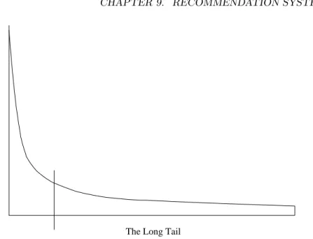
The distinction between the physical and on-line worlds has been called the long tail phenomenon, and it is suggested in Fig. 9.2. The vertical axis representspopularity(the number of times an item is chosen). The items are ordered on the horizontal axis according to their popularity. Physical institu-tions provide only the most popular items to the left of the vertical line, while the corresponding on-line institutions provide the entire range of items: the tail as well as the popular items.
The long-tail phenomenon forces on-line institutions to recommend items to individual users. It is not possible to present all available items to the user, the way physical institutions can. Neither can we expect users to have heard of each of the items they might like.
9.1.3
Applications of Recommendation Systems
We have mentioned several important applications of recommendation systems, but here we shall consolidate the list in a single place.
1. Product Recommendations: Perhaps the most important use of recom-mendation systems is at on-line retailers. We have noted how Amazon or similar on-line vendors strive to present each returning user with some
The Long Tail
Figure 9.2: The long tail: physical institutions can only provide what is popular, while on-line institutions can make everything available
suggestions of products that they might like to buy. These suggestions are not random, but are based on the purchasing decisions made by similar customers or on other techniques we shall discuss in this chapter. 2. Movie Recommendations: Netflix offers its customers recommendations
of movies they might like. These recommendations are based on ratings provided by users, much like the ratings suggested in the example utility matrix of Fig. 9.1. The importance of predicting ratings accurately is so high, that Netflix offered a prize of one million dollars for the first algorithm that could beat its own recommendation system by 10%.1
The prize was finally won in 2009, by a team of researchers called “Bellkor’s Pragmatic Chaos,” after over three years of competition.
3. News Articles: News services have attempted to identify articles of in-terest to readers, based on the articles that they have read in the past. The similarity might be based on the similarity of important words in the documents, or on the articles that are read by people with similar reading tastes. The same principles apply to recommending blogs from among the millions of blogs available, videos on YouTube, or other sites where content is provided regularly.
1
To be exact, the algorithm had to have a root-mean-square error (RMSE) that was 10% less than the RMSE of the Netflix algorithm on a test set taken from actual ratings of Netflix users. To develop an algorithm, contestants were given a training set of data, also taken from actual Netflix data.
Into Thin Air
and
Touching the Void
An extreme example of how the long tail, together with a well designed recommendation system can influence events is the story told by Chris An-derson about a book called Touching the Void. This mountain-climbing book was not a big seller in its day, but many years after it was pub-lished, another book on the same topic, called Into Thin Air was pub-lished. Amazon’s recommendation system noticed a few people who bought both books, and started recommendingTouching the Voidto peo-ple who bought, or were considering, Into Thin Air. Had there been no on-line bookseller,Touching the Voidmight never have been seen by poten-tial buyers, but in the on-line world,Touching the Voideventually became very popular in its own right, in fact, more so thanInto Thin Air.
9.1.4
Populating the Utility Matrix
Without a utility matrix, it is almost impossible to recommend items. However, acquiring data from which to build a utility matrix is often difficult. There are two general approaches to discovering the value users place on items.
1. We can ask users to rate items. Movie ratings are generally obtained this way, and some on-line stores try to obtain ratings from their purchasers. Sites providing content, such as some news sites or YouTube also ask users to rate items. This approach is limited in its effectiveness, since generally users are unwilling to provide responses, and the information from those who do may be biased by the very fact that it comes from people willing to provide ratings.
2. We can make inferences from users’ behavior. Most obviously, if a user buys a product at Amazon, watches a movie on YouTube, or reads a news article, then the user can be said to “like” this item. Note that this sort of rating system really has only one value: 1 means that the user likes the item. Often, we find a utility matrix with this kind of data shown with 0’s rather than blanks where the user has not purchased or viewed the item. However, in this case 0 is not a lower rating than 1; it is no rating at all. More generally, one can infer interest from behavior other than purchasing. For example, if an Amazon customer views information about an item, we can infer that they are interested in the item, even if they don’t buy it.
9.2
Content-Based Recommendations
As we mentioned at the beginning of the chapter, there are two basic architec-tures for a recommendation system:
1. Content-Based systems focus on properties of items. Similarity of items is determined by measuring the similarity in their properties.
2. Collaborative-Filtering systems focus on the relationship between users and items. Similarity of items is determined by the similarity of the ratings of those items by the users who have rated both items.
In this section, we focus on content-based recommendation systems. The next section will cover collaborative filtering.
9.2.1
Item Profiles
In a content-based system, we must construct for each item a profile, which is a record or collection of records representing important characteristics of that item. In simple cases, the profile consists of some characteristics of the item that are easily discovered. For example, consider the features of a movie that might be relevant to a recommendation system.
1. The set of actors of the movie. Some viewers prefer movies with their favorite actors.
2. The director. Some viewers have a preference for the work of certain directors.
3. The year in which the movie was made. Some viewers prefer old movies; others watch only the latest releases.
4. The genre or general type of movie. Some viewers like only comedies, others dramas or romances.
There are many other features of movies that could be used as well. Except for the last, genre, the information is readily available from descriptions of movies. Genre is a vaguer concept. However, movie reviews generally assign a genre from a set of commonly used terms. For example the Internet Movie Database (IMDB) assigns a genre or genres to every movie. We shall discuss mechanical construction of genres in Section 9.3.3.
Many other classes of items also allow us to obtain features from available data, even if that data must at some point be entered by hand. For instance, products often have descriptions written by the manufacturer, giving features relevant to that class of product (e.g., the screen size and cabinet color for a TV). Books have descriptions similar to those for movies, so we can obtain features such as author, year of publication, and genre. Music products such as CD’s and MP3 downloads have available features such as artist, composer, and genre.
9.2.2
Discovering Features of Documents
There are other classes of items where it is not immediately apparent what the values of features should be. We shall consider two of them: document collec-tions and images. Documents present special problems, and we shall discuss the technology for extracting features from documents in this section. Images will be discussed in Section 9.2.3 as an important example where user-supplied features have some hope of success.
There are many kinds of documents for which a recommendation system can be useful. For example, there are many news articles published each day, and we cannot read all of them. A recommendation system can suggest articles on topics a user is interested in, but how can we distinguish among topics? Web pages are also a collection of documents. Can we suggest pages a user might want to see? Likewise, blogs could be recommended to interested users, if we could classify blogs by topics.
Unfortunately, these classes of documents do not tend to have readily avail-able information giving features. A substitute that has been useful in practice is the identification of words that characterize the topic of a document. How we do the identification was outlined in Section 1.3.1. First, eliminate stop words – the several hundred most common words, which tend to say little about the topic of a document. For the remaining words, compute the TF.IDF score for each word in the document. The ones with the highest scores are the words that characterize the document.
We may then take as the features of a document thenwords with the highest TF.IDF scores. It is possible to picknto be the same for all documents, or to letnbe a fixed percentage of the words in the document. We could also choose to make all words whose TF.IDF scores are above a given threshold to be a part of the feature set.
Now, documents are represented by sets of words. Intuitively, we expect these words to express the subjects or main ideas of the document. For example, in a news article, we would expect the words with the highest TF.IDF score to include the names of people discussed in the article, unusual properties of the event described, and the location of the event. To measure the similarity of two documents, there are several natural distance measures we can use:
1. We could use the Jaccard distance between the sets of words (recall Sec-tion 3.5.3).
2. We could use the cosine distance (recall Section 3.5.4) between the sets, treated as vectors.
To compute the cosine distance in option (2), think of the sets of high-TF.IDF words as a vector, with one component for each possible word. The vector has 1 if the word is in the set and 0 if not. Since between two docu-ments there are only a finite number of words among their two sets, the infinite dimensionality of the vectors is unimportant. Almost all components are 0 in
Two Kinds of Document Similarity
Recall that in Section 3.4 we gave a method for finding documents that were “similar,” using shingling, minhashing, and LSH. There, the notion of similarity was lexical – documents are similar if they contain large, identical sequences of characters. For recommendation systems, the notion of similarity is different. We are interested only in the occurrences of many important words in both documents, even if there is little lexical similarity between the documents. However, the methodology for finding similar documents remains almost the same. Once we have a distance measure, either Jaccard or cosine, we can use minhashing (for Jaccard) or random hyperplanes (for cosine distance; see Section 3.7.2) feeding data to an LSH algorithm to find the pairs of documents that are similar in the sense of sharing many common keywords.
both, and 0’s do not impact the value of the dot product. To be precise, the dot product is the size of the intersection of the two sets of words, and the lengths of the vectors are the square roots of the numbers of words in each set. That calculation lets us compute the cosine of the angle between the vectors as the dot product divided by the product of the vector lengths.
9.2.3
Obtaining Item Features From Tags
Let us consider a database of images as an example of a way that features have been obtained for items. The problem with images is that their data, typically an array of pixels, does not tell us anything useful about their features. We can calculate simple properties of pixels, such as the average amount of red in the picture, but few users are looking for red pictures or especially like red pictures. There have been a number of attempts to obtain information about features of items by inviting users to tag the items by entering words or phrases that describe the item. Thus, one picture with a lot of red might be tagged “Tianan-men Square,” while another is tagged “sunset at Malibu.” The distinction is not something that could be discovered by existing image-analysis programs.
Almost any kind of data can have its features described by tags. One of the earliest attempts to tag massive amounts of data was the site del.icio.us, later bought by Yahoo!, which invited users to tag Web pages. The goal of this tagging was to make a new method of search available, where users entered a set of tags as their search query, and the system retrieved the Web pages that had been tagged that way. However, it is also possible to use the tags as a recommendation system. If it is observed that a user retrieves or bookmarks many pages with a certain set of tags, then we can recommend other pages with the same tags.
Tags from Computer Games
An interesting direction for encouraging tagging is the “games” approach pioneered by Luis von Ahn. He enabled two players to collaborate on the tag for an image. In rounds, they would suggest a tag, and the tags would be exchanged. If they agreed, then they “won,” and if not, they would play another round with the same image, trying to agree simultaneously on a tag. While an innovative direction to try, it is questionable whether sufficient public interest can be generated to produce enough free work to satisfy the needs for tagged data.
process only works if users are willing to take the trouble to create the tags, and there are enough tags that occasional erroneous ones will not bias the system too much.
9.2.4
Representing Item Profiles
Our ultimate goal for content-based recommendation is to create both an item profile consisting of feature-value pairs and a user profile summarizing the pref-erences of the user, based of their row of the utility matrix. In Section 9.2.2 we suggested how an item profile could be constructed. We imagined a vector of 0’s and 1’s, where a 1 represented the occurrence of a high-TF.IDF word in the document. Since features for documents were all words, it was easy to represent profiles this way.
We shall try to generalize this vector approach to all sorts of features. It is easy to do so for features that are sets of discrete values. For example, if one feature of movies is the set of actors, then imagine that there is a component for each actor, with 1 if the actor is in the movie, and 0 if not. Likewise, we can have a component for each possible director, and each possible genre. All these features can be represented using only 0’s and 1’s.
There is another class of features that is not readily represented by boolean vectors: those features that are numerical. For instance, we might take the average rating for movies to be a feature,2
and this average is a real number. It does not make sense to have one component for each of the possible average ratings, and doing so would cause us to lose the structure implicit in numbers. That is, two ratings that are close but not identical should be considered more similar than widely differing ratings. Likewise, numerical features of products, such as screen size or disk capacity for PC’s, should be considered similar if their values do not differ greatly.
Numerical features should be represented by single components of vectors representing items. These components hold the exact value of that feature.
2
There is no harm if some components of the vectors are boolean and others are real-valued or integer-valued. We can still compute the cosine distance between vectors, although if we do so, we should give some thought to the appropri-ate scaling of the nonboolean components, so that they neither dominappropri-ate the calculation nor are they irrelevant.
Example 9.2 : Suppose the only features of movies are the set of actors and the average rating. Consider two movies with five actors each. Two of the actors are in both movies. Also, one movie has an average rating of 3 and the other an average of 4. The vectors look something like
0 1 1 0 1 1 0 1 3α
1 1 0 1 0 1 1 0 4α
However, there are in principle an infinite number of additional components, each with 0’s for both vectors, representing all the possible actors that neither movie has. Since cosine distance of vectors is not affected by components in which both vectors have 0, we need not worry about the effect of actors that are in neither movie.
The last component shown represents the average rating. We have shown it as having an unknown scaling factorα. In terms ofα, we can compute the cosine of the angle between the vectors. The dot product is 2 + 12α2
, and the lengths of the vectors are √5 + 9α2
and √5 + 16α2
. Thus, the cosine of the angle between the vectors is
2 + 12α2
√
25 + 125α2+ 144α4
If we choose α= 1, that is, we take the average ratings as they are, then the value of the above expression is 0.816. If we useα= 2, that is, we double the ratings, then the cosine is 0.940. That is, the vectors appear much closer in direction than if we useα= 1. Likewise, if we useα= 1/2, then the cosine is 0.619, making the vectors look quite different. We cannot tell which value of αis “right,” but we see that the choice of scaling factor for numerical features affects our decision about how similar items are. 2
9.2.5
User Profiles
We not only need to create vectors describing items; we need to create vectors with the same components that describe the user’s preferences. We have the utility matrix representing the connection between users and items. Recall the nonblank matrix entries could be just 1’s representing user purchases or a similar connection, or they could be arbitrary numbers representing a rating or degree of affection that the the user has for the item.
With this information, the best estimate we can make regarding which items the user likes is some aggregation of the profiles of those items. If the utility matrix has only 1’s, then the natural aggregate is the average of the components
of the vectors representing the item profiles for the items in which the utility matrix has 1 for that user.
Example 9.3 : Suppose items are movies, represented by boolean profiles with components corresponding to actors. Also, the utility matrix has a 1 if the user has seen the movie and is blank otherwise. If 20% of the movies that user U likes have Julia Roberts as one of the actors, then the user profile for U will have 0.2 in the component for Julia Roberts. 2
If the utility matrix is not boolean, e.g., ratings 1–5, then we can weight the vectors representing the profiles of items by the utility value. It makes sense to normalize the utilities by subtracting the average value for a user. That way, we get negative weights for items with a below-average rating, and positive weights for items with above-average ratings. That effect will prove useful when we discuss in Section 9.2.6 how to find items that a user should like.
Example 9.4 : Consider the same movie information as in Example 9.3, but now suppose the utility matrix has nonblank entries that are ratings in the 1–5 range. Suppose user U gives an average rating of 3. There are three movies with Julia Roberts as an actor, and those movies got ratings of 3, 4, and 5. Then in the user profile ofU, the component for Julia Roberts will have value that is the average of 3−3, 4−3, and 5−3, that is, a value of 1.
On the other hand, userV gives an average rating of 4, and has also rated three movies with Julia Roberts (it doesn’t matter whether or not they are the same three movies U rated). User V gives these three movies ratings of 2, 3, and 5. The user profile for V has, in the component for Julia Roberts, the average of 2−4, 3−4, and 5−4, that is, the value−2/3. 2
9.2.6
Recommending Items to Users Based on Content
With profile vectors for both users and items, we can estimate the degree to which a user would prefer an item by computing the cosine distance between the user’s and item’s vectors. As in Example 9.2, we may wish to scale var-ious components whose values are not boolean. The random-hyperplane and locality-sensitive-hashing techniques can be used to place (just) item profiles in buckets. In that way, given a user to whom we want to recommend some items, we can apply the same two techniques – random hyperplanes and LSH – to determine in which buckets we must look for items that might have a small cosine distance from the user.Example 9.5 : Consider first the data of Example 9.3. The user’s profile will have components for actors proportional to the likelihood that the actor will appear in a movie the user likes. Thus, the highest recommendations (lowest cosine distance) belong to the movies with lots of actors that appear in many
of the movies the user likes. As long as actors are the only information we have about features of movies, that is probably the best we can do.3
Now, consider Example 9.4. There, we observed that the vector for a user will have positive numbers for actors that tend to appear in movies the user likes and negative numbers for actors that tend to appear in movies the user doesn’t like. Consider a movie with many actors the user likes, and only a few or none that the user doesn’t like. The cosine of the angle between the user’s and movie’s vectors will be a large positive fraction. That implies an angle close to 0, and therefore a small cosine distance between the vectors.
Next, consider a movie with about as many actors that the user likes as those the user doesn’t like. In this situation, the cosine of the angle between the user and movie is around 0, and therefore the angle between the two vectors is around 90 degrees. Finally, consider a movie with mostly actors the user doesn’t like. In that case, the cosine will be a large negative fraction, and the angle between the two vectors will be close to 180 degrees – the maximum possible cosine distance. 2
9.2.7
Classification Algorithms
A completely different approach to a recommendation system using item profiles and utility matrices is to treat the problem as one of machine learning. Regard the given data as a training set, and for each user, build a classifier that predicts the rating of all items. There are a great number of different classifiers, and it is not our purpose to teach this subject here. However, you should be aware of the option of developing a classifier for recommendation, so we shall discuss one common classifier – decision trees – briefly.
A decision tree is a collection of nodes, arranged as a binary tree. The leaves render decisions; in our case, the decision would be “likes” or “doesn’t like.” Each interior node is a condition on the objects being classified; in our case the condition would be a predicate involving one or more features of an item.
To classify an item, we start at the root, and apply the predicate at the root to the item. If the predicate is true, go to the left child, and if it is false, go to the right child. Then repeat the same process at the node visited, until a leaf is reached. That leaf classifies the item as liked or not.
Construction of a decision tree requires selection of a predicate for each interior node. There are many ways of picking the best predicate, but they all try to arrange that one of the children gets all or most of the positive examples in the training set (i.e, the items that the given user likes, in our case) and the other child gets all or most of the negative examples (the items this user does not like).
3
Note that the fact all user-vector components will be small fractions does not affect the recommendation, since the cosine calculation involves dividing by the length of each vector. That is, user vectors will tend to be much shorter than movie vectors, but only the direction of vectors matters.
Once we have selected a predicate for a node N, we divide the items into the two groups: those that satisfy the predicate and those that do not. For each group, we again find the predicate that best separates the positive and negative examples in that group. These predicates are assigned to the children ofN. This process of dividing the examples and building children can proceed to any number of levels. We can stop, and create a leaf, if the group of items for a node is homogeneous; i.e., they are all positive or all negative examples.
However, we may wish to stop and create a leaf with the majority decision for a group, even if the group contains both positive and negative examples. The reason is that the statistical significance of a small group may not be high enough to rely on. For that reason a variant strategy is to create anensembleof decision trees, each using different predicates, but allow the trees to be deeper than what the available data justifies. Such trees are called overfitted. To classify an item, apply all the trees in the ensemble, and let them vote on the outcome. We shall not consider this option here, but give a simple hypothetical example of a decision tree.
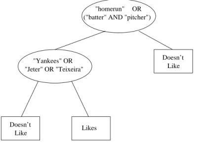
Example 9.6 : Suppose our items are news articles, and features are the high-TF.IDF words (keywords) in those documents. Further suppose there is a user Uwho likes articles about baseball, except articles about the New York Yankees. The row of the utility matrix forU has 1 ifU has read the article and is blank if not. We shall take the 1’s as “like” and the blanks as “doesn’t like.” Predicates will be boolean expressions of keywords.
Since U generally likes baseball, we might find that the best predicate for the root is “homerun” OR (“batter” AND “pitcher”). Items that satisfy the predicate will tend to be positive examples (articles with 1 in the row forU in the utility matrix), and items that fail to satisfy the predicate will tend to be negative examples (blanks in the utility-matrix row for U). Figure 9.3 shows the root as well as the rest of the decision tree.
Suppose that the group of articles that do not satisfy the predicate includes sufficiently few positive examples that we can conclude all of these items are in the “don’t-like” class. We may then put a leaf with decision “don’t like” as the right child of the root. However, the articles that satisfy the predicate includes a number of articles that userU doesn’t like; these are the articles that mention the Yankees. Thus, at the left child of the root, we build another predicate. We might find that the predicate “Yankees” OR “Jeter” OR “Teixeira” is the best possible indicator of an article about baseball and about the Yankees. Thus, we see in Fig. 9.3 the left child of the root, which applies this predicate. Both children of this node are leaves, since we may suppose that the items satisfying this predicate are predominantly negative and those not satisfying it are predominantly positive. 2
Unfortunately, classifiers of all types tend to take a long time to construct. For instance, if we wish to use decision trees, we need one tree per user. Con-structing a tree not only requires that we look at all the item profiles, but we
("batter" AND "pitcher") "homerun" OR
"Yankees" OR "Jeter" OR "Teixeira"
Doesn’t Like
Doesn’t Like
Likes
Figure 9.3: A decision tree
have to consider many different predicates, which could involve complex com-binations of features. Thus, this approach tends to be used only for relatively small problem sizes.
9.2.8
Exercises for Section 9.2
Exercise 9.2.1 : Three computers, A, B, andC, have the numerical features listed below:
Feature A B C
Processor Speed 3.06 2.68 2.92
Disk Size 500 320 640
Main-Memory Size 6 4 6
We may imagine these values as defining a vector for each computer; for in-stance,A’s vector is [3.06,500,6]. We can compute the cosine distance between any two of the vectors, but if we do not scale the components, then the disk size will dominate and make differences in the other components essentially in-visible. Let us use 1 as the scale factor for processor speed,αfor the disk size, andβ for the main memory size.
(a) In terms ofαandβ, compute the cosines of the angles between the vectors for each pair of the three computers.
(b) What are the angles between the vectors ifα=β = 1?
!(d) One fair way of selecting scale factors is to make each inversely propor-tional to the average value in its component. What would be the values ofαandβ, and what would be the angles between the vectors?
Exercise 9.2.2 : An alternative way of scaling components of a vector is to begin by normalizing the vectors. That is, compute the average for each com-ponent and subtract it from that comcom-ponent’s value in each of the vectors.
(a) Normalize the vectors for the three computers described in Exercise 9.2.1.
!!(b) This question does not require difficult calculation, but it requires some serious thought about what angles between vectors mean. When all com-ponents are nonnegative, as they are in the data of Exercise 9.2.1, no vectors can have an angle greater than 90 degrees. However, when we normalize vectors, we can (and must) get some negative components, so the angles can now be anything, that is, 0 to 180 degrees. Moreover, averages are now 0 in every component, so the suggestion in part (d) of Exercise 9.2.1 that we should scale in inverse proportion to the average makes no sense. Suggest a way of finding an appropriate scale for each component of normalized vectors. How would you interpret a large or small angle between normalized vectors? What would the angles be for the normalized vectors derived from the data in Exercise 9.2.1?
Exercise 9.2.3 : A certain user has rated the three computers of Exercise 9.2.1 as follows: A: 4 stars,B: 2 stars,C: 5 stars.
(a) Normalize the ratings for this user.
(b) Compute a user profile for the user, with components for processor speed, disk size, and main memory size, based on the data of Exercise 9.2.1.
9.3
Collaborative Filtering
We shall now take up a significantly different approach to recommendation. Instead of using features of items to determine their similarity, we focus on the similarity of the user ratings for two items. That is, in place of the item-profile vector for an item, we use its column in the utility matrix. Further, instead of contriving a profile vector for users, we represent them by their rows in the utility matrix. Users are similar if their vectors are close according to some distance measure such as Jaccard or cosine distance. Recommendation for a userU is then made by looking at the users that are most similar toU in this sense, and recommending items that these users like. The process of identifying similar users and recommending what similar users like is called collaborative filtering.
9.3.1
Measuring Similarity
The first question we must deal with is how to measure similarity of users or items from their rows or columns in the utility matrix. We have reproduced Fig. 9.1 here as Fig. 9.4. This data is too small to draw any reliable conclusions, but its small size will make clear some of the pitfalls in picking a distance measure. Observe specifically the users A and C. They rated two movies in common, but they appear to have almost diametrically opposite opinions of these movies. We would expect that a good distance measure would make them rather far apart. Here are some alternative measures to consider.
HP1 HP2 HP3 TW SW1 SW2 SW3
A 4 5 1
B 5 5 4
C 2 4 5
D 3 3
Figure 9.4: The utility matrix introduced in Fig. 9.1
Jaccard Distance
We could ignore values in the matrix and focus only on the sets of items rated. If the utility matrix only reflected purchases, this measure would be a good one to choose. However, when utilities are more detailed ratings, the Jaccard distance loses important information.
Example 9.7 : A and B have an intersection of size 1 and a union of size 5. Thus, their Jaccard similarity is 1/5, and their Jaccard distance is 4/5; i.e., they are very far apart. In comparison, A andC have a Jaccard similarity of 2/4, so their Jaccard distance is the same, 1/2. Thus, A appears closer toC than to B. Yet that conclusion seems intuitively wrong. AandC disagree on the two movies they both watched, whileAandB seem both to have liked the one movie they watched in common. 2
Cosine Distance
We can treat blanks as a 0 value. This choice is questionable, since it has the effect of treating the lack of a rating as more similar to disliking the movie than liking it.
Example 9.8 : The cosine of the angle betweenAandB is 4×5
√
The cosine of the angle betweenAand Cis 5×2 + 1×4 √
42+ 52+ 12√22+ 42+ 52 = 0.322
Since a larger (positive) cosine implies a smaller angle and therefore a smaller distance, this measure tells us thatAis slightly closer toB than to C. 2
Rounding the Data
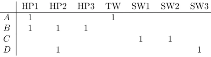
We could try to eliminate the apparent similarity between movies a user rates highly and those with low scores by rounding the ratings. For instance, we could consider ratings of 3, 4, and 5 as a “1” and consider ratings 1 and 2 as unrated. The utility matrix would then look as in Fig. 9.5. Now, the Jaccard distance betweenAandB is 3/4, while betweenAandCit is 1; i.e.,C appears further from Athan B does, which is intuitively correct. Applying cosine distance to Fig. 9.5 allows us to draw the same conclusion.
HP1 HP2 HP3 TW SW1 SW2 SW3
A 1 1
B 1 1 1
C 1 1
D 1 1
Figure 9.5: Utilities of 3, 4, and 5 have been replaced by 1, while ratings of 1 and 2 are omitted
Normalizing Ratings
If we normalize ratings, by subtracting from each rating the average rating of that user, we turn low ratings into negative numbers and high ratings into positive numbers. If we then take the cosine distance, we find that users with opposite views of the movies they viewed in common will have vectors in almost opposite directions, and can be considered as far apart as possible. However, users with similar opinions about the movies rated in common will have a relatively small angle between them.
Example 9.9 : Figure 9.6 shows the matrix of Fig. 9.4 with all ratings nor-malized. An interesting effect is thatD’s ratings have effectively disappeared, because a 0 is the same as a blank when cosine distance is computed. Note that D gave only 3’s and did not differentiate among movies, so it is quite possible thatD’s opinions are not worth taking seriously.
Let us compute the cosine of the angle betweenAand B: (2/3)×(1/3)
p
(2/3)2+ (5/3)2+ (
−7/3)2p(1/3)2+ (1/3)2+ (−2/3)2
HP1 HP2 HP3 TW SW1 SW2 SW3 A 2/3 5/3 −7/3
B 1/3 1/3 −2/3
C −5/3 1/3 4/3
D 0 0
Figure 9.6: The utility matrix introduced in Fig. 9.1 The cosine of the angle between betweenAandC is
(5/3)×(−5/3) + (−7/3)×(1/3) p
(2/3)2+ (5/3)2+ (
−7/3)2p(−5/3)2+ (1/3)2+ (4/3)2
=−0.559 Notice that under this measure,A andC are much further apart thanA and B, and neither pair is very close. Both these observations make intuitive sense, given thatAandCdisagree on the two movies they rated in common, whileA andB give similar scores to the one movie they rated in common. 2
9.3.2
The Duality of Similarity
The utility matrix can be viewed as telling us about users or about items, or both. It is important to realize that any of the techniques we suggested in Section 9.3.1 for finding similar users can be used on columns of the utility matrix to find similar items. There are two ways in which the symmetry is broken in practice.
1. We can use information about users to recommend items. That is, given a user, we can find some number of the most similar users, perhaps using the techniques of Chapter 3. We can base our recommendation on the decisions made by these similar users, e.g., recommend the items that the greatest number of them have purchased or rated highly. However, there is no symmetry. Even if we find pairs of similar items, we need to take an additional step in order to recommend items to users. This point is explored further at the end of this subsection.
2. There is a difference in the typical behavior of users and items, as it pertains to similarity. Intuitively, items tend to be classifiable in simple terms. For example, music tends to belong to a single genre. It is impossi-ble, e.g., for a piece of music to be both 60’s rock and 1700’s baroque. On the other hand, there are individuals who like both 60’s rock and 1700’s baroque, and who buy examples of both types of music. The consequence is that it is easier to discover items that are similar because they belong to the same genre, than it is to detect that two users are similar because they prefer one genre in common, while each also likes some genres that the other doesn’t care for.
As we suggested in (1) above, one way of predicting the value of the utility-matrix entry for userUand itemIis to find thenusers (for some predetermined n) most similar toU and average their ratings for item I, counting only those among thensimilar users who have ratedI. It is generally better to normalize the matrix first. That is, for each of the nusers subtract their average rating for items from their rating for i. Average the difference for those users who have ratedI, and then add this average to the average rating thatU gives for all items. This normalization adjusts the estimate in the case thatU tends to give very high or very low ratings, or a large fraction of the similar users who ratedI(of which there may be only a few) are users who tend to rate very high or very low.
Dually, we can use item similarity to estimate the entry for userU and item I. Find themitems most similar toI, for somem, and take the average rating, among themitems, of the ratings thatU has given. As for user-user similarity, we consider only those items among themthatU has rated, and it is probably wise to normalize item ratings first.
Note that whichever approach to estimating entries in the utility matrix we use, it is not sufficient to find only one entry. In order to recommend items to a userU, we need to estimate every entry in the row of the utility matrix for U, or at least find all or most of the entries in that row that are blank but have a high estimated value. There is a tradeoff regarding whether we should work from similar users or similar items.
• If we find similar users, then we only have to do the process once for user U. From the set of similar users we can estimate all the blanks in the utility matrix forU. If we work from similar items, we have to compute similar items for almost all items, before we can estimate the row for U.
• On the other hand, item-item similarity often provides more reliable in-formation, because of the phenomenon observed above, namely that it is easier to find items of the same genre than it is to find users that like only items of a single genre.
Whichever method we choose, we should precompute preferred items for each user, rather than waiting until we need to make a decision. Since the utility matrix evolves slowly, it is generally sufficient to compute it infrequently and assume that it remains fixed between recomputations.
9.3.3
Clustering Users and Items
It is hard to detect similarity among either items or users, because we have little information about user-item pairs in the sparse utility matrix. In the perspective of Section 9.3.2, even if two items belong to the same genre, there are likely to be very few users who bought or rated both. Likewise, even if two users both like a genre or genres, they may not have bought any items in common.
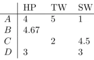
One way of dealing with this pitfall is to cluster items and/or users. Select any of the distance measures suggested in Section 9.3.1, or any other distance measure, and use it to perform a clustering of, say, items. Any of the methods suggested in Chapter 7 can be used. However, we shall see that there may be little reason to try to cluster into a small number of clusters immediately. Rather, a hierarchical approach, where we leave many clusters unmerged may suffice as a first step. For example, we might leave half as many clusters as there are items.
HP TW SW
A 4 5 1 B 4.67
C 2 4.5
D 3 3
Figure 9.7: Utility matrix for users and clusters of items
Example 9.10 : Figure 9.7 shows what happens to the utility matrix of Fig. 9.4 if we manage to cluster the three Harry-Potter movies into one cluster, denoted HP, and also cluster the three Star-Wars movies into one cluster SW. 2
Having clustered items to an extent, we can revise the utility matrix so the columns represent clusters of items, and the entry for userU and clusterC is the average rating thatU gave to those members of clusterC that U did rate. Note that U may have rated none of the cluster members, in which case the entry forU andC is still blank.
We can use this revised utility matrix to cluster users, again using the dis-tance measure we consider most appropriate. Use a clustering algorithm that again leaves many clusters, e.g., half as many clusters as there are users. Re-vise the utility matrix, so the rows correspond to clusters of users, just as the columns correspond to clusters of items. As for item-clusters, compute the entry for a user cluster by averaging the ratings of the users in the cluster.
Now, this process can be repeated several times if we like. That is, we can cluster the item clusters and again merge the columns of the utility matrix that belong to one cluster. We can then turn to the users again, and cluster the user clusters. The process can repeat until we have an intuitively reasonable number of clusters of each kind.
Once we have clustered the users and/or items to the desired extent and computed the cluster-cluster utility matrix, we can estimate entries in the orig-inal utility matrix as follows. Suppose we want to predict the entry for userU and itemI:
(a) Find the clusters to whichU andI belong, say clustersCandD, respec-tively.
(b) If the entry in the cluster-cluster utility matrix forCandDis something other than blank, use this value as the estimated value for theU–Ientry in the original utility matrix.
(c) If the entry forC–Dis blank, then use the method outlined in Section 9.3.2 to estimate that entry by considering clusters similar to CorD. Use the resulting estimate as the estimate for theU-I entry.
9.3.4
Exercises for Section 9.3
a b c d e f g h A 4 5 5 1 3 2 B 3 4 3 1 2 1 C 2 1 3 4 5 3
Figure 9.8: A utility matrix for exercises
Exercise 9.3.1 : Figure 9.8 is a utility matrix, representing the ratings, on a 1–5 star scale, of eight items,athroughh, by three usersA,B, andC. Compute the following from the data of this matrix.
(a) Treating the utility matrix as boolean, compute the Jaccard distance be-tween each pair of users.
(b) Repeat Part (a), but use the cosine distance.
(c) Treat ratings of 3, 4, and 5 as 1 and 1, 2, and blank as 0. Compute the Jaccard distance between each pair of users.
(d) Repeat Part (c), but use the cosine distance.
(e) Normalize the matrix by subtracting from each nonblank entry the average value for its user.
(f) Using the normalized matrix from Part (e), compute the cosine distance between each pair of users.
Exercise 9.3.2 : In this exercise, we cluster items in the matrix of Fig. 9.8. Do the following steps.
(a) Cluster the eight items hierarchically into four clusters. The following method should be used to cluster. Replace all 3’s, 4’s, and 5’s by 1 and replace 1’s, 2’s, and blanks by 0. use the Jaccard distance to measure the distance between the resulting column vectors. For clusters of more than one element, take the distance between clusters to be the minimum distance between pairs of elements, one from each cluster.
(b) Then, construct from the original matrix of Fig. 9.8 a new matrix whose rows correspond to users, as before, and whose columns correspond to clusters. Compute the entry for a user and cluster of items by averaging the nonblank entries for that user and all the items in the cluster. (c) Compute the cosine distance between each pair of users, according to your
matrix from Part (b).
9.4
Dimensionality Reduction
An entirely different approach to estimating the blank entries in the utility matrix is to conjecture that the utility matrix is actually the product of two long, thin matrices. This view makes sense if there are a relatively small set of features of items and users that determine the reaction of most users to most items. In this section, we sketch one approach to discovering two such matrices; the approach is called “UV-decomposition,” and it is an instance of a more general theory called SVD (singular-value decomposition).
9.4.1
UV-Decomposition
Consider movies as a case in point. Most users respond to a small number of features; they like certain genres, they may have certain famous actors or actresses that they like, and perhaps there are a few directors with a significant following. If we start with the utility matrixM, with nrows and m columns (i.e., there are nusers and mitems), then we might be able to find a matrix U with n rows and d columns and a matrix V with d rows and m columns, such that U V closely approximates M in those entries whereM is nonblank. If so, then we have established that there are d dimensions that allow us to characterize both users and items closely. We can then use the entry in the product U V to estimate the corresponding blank entry in utility matrix M. This process is calledUV-decompositionofM.
5 2 4 4 3
3 1 2 4 1
2 3 1 4
2 5 4 3 5
4 4 5 4 =
u11 u12
u21 u22
u31 u32
u41 u42
u51 u52
×
v11 v12 v13 v14 v15
v21 v22 v23 v24 v25
Figure 9.9: UV-decomposition of matrixM
Example 9.11 : We shall use as a running example a 5-by-5 matrixM with all but two of its entries known. We wish to decompose M into a 5-by-2 and 2-by-5 matrix, U and V, respectively. The matrices M, U, and V are shown in Fig. 9.9 with the known entries of M indicated and the matrices U and
V shown with their entries as variables to be determined. This example is essentially the smallest nontrivial case where there are more known entries than there are entries in U and V combined, and we therefore can expect that the best decomposition will not yield a product that agrees exactly in the nonblank entries ofM. 2
9.4.2
Root-Mean-Square Error
While we can pick among several measures of how close the productU V is to M, the typical choice is the root-mean-square error (RMSE), where we
1. Sum, over all nonblank entries inM the square of the difference between that entry and the corresponding entry in the productU V.
2. Take the mean (average) of these squares by dividing by the number of terms in the sum (i.e., the number of nonblank entries inM).
3. Take the square root of the mean.
Minimizing the sum of the squares is the same as minimizing the square root of the average square, so we generally omit the last two steps in our running example. 1 1 1 1 1 1 1 1 1 1 ×
1 1 1 1 1 1 1 1 1 1
=
2 2 2 2 2
2 2 2 2 2
2 2 2 2 2
2 2 2 2 2
2 2 2 2 2
Figure 9.10: MatricesU andV with all entries 1
Example 9.12 : Suppose we guess thatU andV should each have entries that are all 1’s, as shown in Fig. 9.10. This is a poor guess, since the product, consisting of all 2’s, has entries that are much below the average of the entries in M. Nonetheless, we can compute the RMSE for this U and V; in fact the regularity in the entries makes the calculation especially easy to follow. Consider the first rows ofM andU V. We subtract 2 (each entry inU V) from the entries in the first row ofM, to get 3,0,2,2,1. We square and sum these to get 18. In the second row, we do the same to get 1,−1,0,2,−1, square and sum to get 7. In the third row, the second column is blank, so that entry is ignored when computing the RMSE. The differences are 0,1,−1,2 and the sum of squares is 6. For the fourth row, the differences are 0,3,2,1,3 and the sum of squares is 23. The fifth row has a blank entry in the last column, so the differences are 2,2,3,2 and the sum of squares is 21. When we sum the sums from each of the five rows, we get 18 + 7 + 6 + 23 + 21 = 75. Generally, we shall
stop at this point, but if we want to compute the true RMSE, we divide by 23 (the number of nonblank entries inM) and take the square root. In this case p
75/23 = 1.806 is the RMSE. 2
9.4.3
Incremental Computation of a UV-Decomposition
Finding the UV-decomposition with the least RMSE involves starting with some arbitrarily chosen U andV, and repeatedly adjusting U and V to make the RMSE smaller. We shall consider only adjustments to a single element of U or V, although in principle, one could make more complex adjustments. Whatever adjustments we allow, in a typical example there will be many lo-cal minima – matrices U and V such that no allowable adjustment reduces the RMSE. Unfortunately, only one of these local minima will be the global minimum – the matricesU andV that produce the least possible RMSE. To increase our chances of finding the global minimum, we need to pick many dif-ferent starting points, that is, difdif-ferent choices of the initial matricesU andV. However, there is never a guarantee that our best local minimum will be the global minimum.We shall start with theU andV of Fig. 9.10, where all entries are 1, and do a few adjustments to some of the entries, finding the values of those entries that give the largest possible improvement to the RMSE. From these examples, the general calculation should become obvious, but we shall follow the examples by the formula for minimizing the RMSE by changing a single entry. In what follows, we shall refer to entries ofU andV by their variable names u11, and
so on, as given in Fig. 9.9.
Example 9.13 : Suppose we start withU andV as in Fig. 9.10, and we decide to alteru11 to reduce the RMSE as much as possible. Let the value ofu11 be
x. Then the new U andV can be expressed as in Fig. 9.11.
x 1 1 1 1 1 1 1 1 1 ×
1 1 1 1 1
1 1 1 1 1
=
x+ 1 x+ 1 x+ 1 x+ 1 x+ 1
2 2 2 2 2
2 2 2 2 2
2 2 2 2 2
2 2 2 2 2
Figure 9.11: Makingu11 a variable
Notice that the only entries of the product that have changed are those in the first row. Thus, when we compare U V with M, the only change to the RMSE comes from the first row. The contribution to the sum of squares from the first row is
5−(x+ 1)
2
+ 2−(x+ 1)
2
+ 4−(x+ 1)
2
+ 4−(x+ 1)
2
+ 3−(x+ 1)
This sum simplifies to
(4−x)2+ (1−x)2+ (3−x)2+ (3−x)2+ (2−x)2
We want the value ofxthat minimizes the sum, so we take the derivative and set that equal to 0, as:
−2× (4−x) + (1−x) + (3−x) + (3−x) + (2−x)= 0 or−2×(13−5x) = 0, from which it follows thatx= 2.6.
2.6 1 1 1 1 1 1 1 1 1 ×
1 1 1 1 1
1 1 1 1 1
=
3.6 3.6 3.6 3.6 3.6
2 2 2 2 2
2 2 2 2 2
2 2 2 2 2
2 2 2 2 2
Figure 9.12: The best value foru11 is found to be 2.6
Figure 9.12 showsU andV afteru11has been set to 2.6. Note that the sum
of the squares of the errors in the first row has been reduced from 18 to 5.2, so the total RMSE (ignoring average and square root) has been reduced from 75 to 62.2. 2.6 1 1 1 1 1 1 1 1 1 ×
y 1 1 1 1
1 1 1 1 1
=
2.6y+ 1 3.6 3.6 3.6 3.6 y+ 1 2 2 2 2 y+ 1 2 2 2 2 y+ 1 2 2 2 2 y+ 1 2 2 2 2
Figure 9.13: v11becomes a variabley
Suppose our next entry to vary is v11. Let the value of this entry bey, as
suggested in Fig. 9.13. Only the first column of the product is affected byy, so we need only to compute the sum of the squares of the differences between the entries in the first columns ofM andU V. This sum is
5−(2.6y+ 1)
2
+ 3−(y+ 1)
2
+ 2−(y+ 1)
2
+ 2−(y+ 1)
2
+ 4−(y+ 1)
2
This expression simplifies to
(4−2.6y)2+ (2−y)2+ (1−y)2+ (1−y)2+ (3−y)2
As before, we find the minimum value of this expression by differentiating and equating to 0, as:
2.6 1 1 1 1 1 1 1 1 1 ×
1.617 1 1 1 1
1 1 1 1 1
=
5.204 3.6 3.6 3.6 3.6
2.617 2 2 2 2
2.617 2 2 2 2
2.617 2 2 2 2
2.617 2 2 2 2
Figure 9.14: Replacey by 1.617
The solution foryisy= 17.4/10.76 = 1.617. The improved estimates ofU and V are shown in Fig. 9.14.
We shall do one more change, to illustrate what happens when entries ofM are blank. We shall varyu31, calling it z temporarily. The newU andV are
shown in Fig. 9.15. The value ofzaffects only the entries in the third row.
2 6 6 6 6 4
2.6 1
1 1 z 1 1 1 1 1 3 7 7 7 7 5 × »
1.617 1 1 1 1
1 1 1 1 1
– = 2 6 6 6 6 4
5.204 3.6 3.6 3.6 3.6
2.617 2 2 2 2
1.617z+ 1 z+ 1 z+ 1 z+ 1 z+ 1
2.617 2 2 2 2
2.617 2 2 2 2
3 7 7 7 7 5
Figure 9.15: u31 becomes a variablez
We can express the sum of the squares of the errors as 2−(1.617z+ 1)
2
+ 3−(z+ 1)
2
+ 1−(z+ 1)
2
+ 4−(z+ 1)
2
Note that there is no contribution from the element in the second column of the third row, since this element is blank inM. The expression simplifies to
(1−1.617z)2+ (2−z)2+ (−z)2+ (3−z)2
The usual process of setting the derivative to 0 gives us
−2× 1.617(1−1.617z) + (2−z) + (−z) + (3−z)= 0
whose solution isz= 6.617/5.615 = 1.178. The next estimate of the decompo-sitionU V is shown in Fig. 9.16. 2
9.4.4
Optimizing an Arbitrary Element
Having seen some examples of picking the optimum value for a single element in the matrix U or V, let us now develop the general formula. As before, assume
2 6 6 6 6 4
2.6 1
1 1 1.178 1
1 1 1 1 3 7 7 7 7 5 × »
1.617 1 1 1 1
1 1 1 1 1
– = 2 6 6 6 6 4
5.204 3.6 3.6 3.6 3.6
2.617 2 2 2 2
2.905 2.178 2.178 2.178 2.178
2.617 2 2 2 2
2.617 2 2 2 2
3 7 7 7 7 5
Figure 9.16: Replacez by 1.178
that M is an n-by-m utility matrix with some entries blank, while U and V are matrices of dimensions n-by-dandd-by-m, for some d. We shall use mij,
uij, andvij for the entries in rowiand columnj ofM,U, andV, respectively.
Also, let P = U V, and use pij for the element in row i and column j of the
product matrixP.
Suppose we want to vary ursand find the value of this element that
mini-mizes the RMSE betweenM andU V. Note thatursaffects only the elements
in rowr of the product P =U V. Thus, we need only concern ourselves with the elements
prj= d
X
k=1
urkvkj =
X
k6=s
urkvkj +xvsj
for all values ofj such thatmrj is nonblank. In the expression above, we have
replaced urs, the element we wish to vary, by a variable x, and we use the
convention
• Pk6=sis shorthand for the sum fork= 1,2, . . . , d, except fork=s.
If mrj is a nonblank entry of the matrix M, then the contribution of this
element to the sum of the squares of the errors is (mrj−prj)
2
= mrj− X
k6=s
urkvkj−xvsj
2
We shall use another convention:
• Pj is shorthand for the sum over allj such thatmrj is nonblank.
Then we can write the sum of the squares of the errors that are affected by the value ofx=urs as
X
j
mrj− X
k6=s
urkvkj−xvsj
2
Take the derivative of the above with respect to x, and set it equal to 0, in order to find the value ofxthat minimizes the RMSE. That is,
X
j
−2vsj mrj− X
k6=s
urkvkj−xvsj
= 0
As in the previous examples, the common factor−2 can be dropped. We solve the above equation forx, and get
x= P
jvsj mrj−Pk6=surkvkj
P
jv
2
sj
There is an analogous formula for the optimum value of an element ofV. If we want to varyvrs=y, then the value ofy that minimizes the RMSE is
y= P
iuir mis−
P
k6=ruikvks
P
iu
2
ir
Here, P
i is shorthand for the sum over all i such that mis is nonblank, and
P
k6=r is the sum over all values ofkbetween 1 andd, except fork=r.
9.4.5
Building a Complete UV-Decomposition Algorithm
Now, we have the tools to search for the global optimum decomposition of a utility matrixM. There are four areas where we shall discuss the options.1. Preprocessing of the matrixM. 2. InitializingU andV.
3. Ordering the optimization of the elements ofU andV. 4. Ending the attempt at optimization.
Preprocessing
Because the differences in the quality of items and the rating scales of users are such important factors in determining the missing elements of the matrixM, it is often useful to remove these influences before doing anything else. The idea was introduced in Section 9.3.1. We can subtract from each nonblank element mij the average rating of useri. Then, the resulting matrix can be modified
by subtracting the average rating (in the modified matrix) of itemj. It is also possible to first subtract the average rating of item j and then subtract the average rating of user i in the modified matrix. The results one obtains from doing things in these two different orders need not be the same, but will tend to be close. A third option is to normalize by subtracting frommij the average
of the average rating of useriand itemj, that is, subtracting one half the sum of the user average and the item average.
If we choose to normalize M, then when we make predictions, we need to undo the normalization. That is, if whatever prediction method we use results in estimate e for an element mij of the normalized matrix, then the value
we predict for mij in the true utility matrix is e plus whatever amount was
Initialization
As we mentioned, it is essential that there be some randomness in the way we seek an optimum solution, because the existence of many local minima justifies our running many different optimizations in the hope of reaching the global minimum on at least one run. We can vary the initial values ofU andV, or we can vary the way we seek the optimum (to be discussed next), or both.
A simple starting point forU andV is to give each element the same value, and a good choice for this value is that which gives the elements of the product U V the average of the nonblank elements ofM. Note that if we have normalized M, then this value will necessarily be 0. If we have chosendas the lengths of the short sides ofU andV, andais the average nonblank element ofM, then the elements ofU andV should bep
a/d.
If we want many starting points for U and V, then we can perturb the valuep
a/d randomly and independently for each of the elements. There are many options for how we do the perturbation. We have a choice regarding the distribution of the difference. For example we could add to each element a normally distributed value with mean 0 and some chosen standard deviation. Or we could add a value uniformly chosen from the range−cto +c for somec.
Performing the Optimization
In order to reach a local minimum from a given starting value ofU andV, we need to pick an order in which we visit the elements ofU andV. The simplest thing to do is pick an order, e.g., row-by-row, for the elements of U and V, and visit them in round-robin fashion. Note that just because we optimized an element once does not mean we cannot find a better value for that element after other elements have been adjusted. Thus, we need to visit elements repeatedly, until we have reason to believe that no further improvements are possible.
Alternatively, we can follow many different optimization paths from a single starting value by randomly picking the element to optimize. To make sure that every element is considered in each round, we could instead choose a permuta-tion of the elements and follow that order for every round.
Converging to a Minimum
Ideally, at some point the RMSE becomes 0, and we know we cannot do better. In practice, since there are normally many more nonblank elements inM than there are elements in U and V together, we have no right to expect that we can reduce the RMSE to 0. Thus, we have to detect when there is little benefit to be had in revisiting elements ofU and/orV. We can track the amount of improvement in the RMSE obtained in one round of the optimization, and stop when that improvement falls below a threshold. A small variation is to observe the improvements resulting from the optimization of individual elements, and stop when the maximum improvement during a round is below a threshold.
Gradient Descent
The technique for finding a UV-decomposition discussed in Section 9.4 is an example of gradient descent. We are given some data points – the nonblank elements of the matrix M – and for each data point we find the direction of change that most decreases the error function: the RMSE between the current U V product and M. We shall have much more to say about gradient descent in Section 12.3.4. It is also worth noting that while we have described the method as visiting each nonblank point of M several times until we approach a minimum-error decomposition, that may well be too much work on a large matrix M. Thus, an alternative approach has us look at only a randomly chosen fraction of the data when seeking to minimize the error. This approach, called stochastic gradient descentis discussed in Section 12.3.5.
Avoiding Overfitting
One problem that often arises when performing a UV-decomposition is that we arrive at one of the many local minima that conform well to the given data, but picks up values in the data that don’t reflect well the underlying process that gives rise to the data. That is, although the RMSE may be small on the given data, it doesn’t do well predicting future data. There are several things that can be done to cope with this problem, which is calledoverfittingby statisticians.
1. Avoid favoring the first components to be optimized by only moving the value of a component a fraction of the way, say half way, from its current value toward its optimized value.
2. Stop revisiting elements ofU andV well before the process has converged. 3. Take several different UV decompositions, and when predicting a new entry in the matrix M, take the average of the results of using each decomposition.
9.4.6
Exercises for Section 9.4
Exercise 9.4.1 : Starting with the decomposition of Fig. 9.10, we may choose any of the 20 entries inU orV to optimize first. Perform this first optimization step assuming we choose: (a)u32 (b)v41.
Exercise 9.4.2 : If we wish to start out, as in Fig. 9.10, with all U and V entries set to the same value, what value minimizes the RMSE for the matrix M of our running example?
Exercise 9.4.3 : Starting with the U and V matrices in Fig. 9.16, do the following in order:
(a) Reconsider the value ofu11. Find its new best value, given the changes
that have been made so far. (b) Then choose the best value foru52.
(c) Then choose the best value forv22.
Exercise 9.4.4 : Derive the formula for y (the optimum value of element vrs
given at the end of Section 9.4.4.
Exercise 9.4.5 : Normalize the matrix M of our running example by:
(a) First subtracting from each element the average of its row, and then subtracting from each element the average of its (modified) column. (b) First subtracting from each element the average of its column, and then
subtracting from each element the average of its (modified) row. Are there any differences in the results of (a) and (b)?
9.5
The NetFlix Challenge
A significant boost to research into recommendation systems was given when NetFlix offered a prize of $1,000,000 to the first person or team to beat their own recommendation algorithm, called CineMatch, by 10%. After over three years of work, the prize was awarded in September, 2009.
The NetFlix challenge consisted of a published dataset, giving the ratings by approximately half a million users on (typically small subsets of) approximately 17,000 movies. This data was selected from a larger dataset, and proposed al-gorithms were tested on their ability to predict the ratings in a secret remainder of the larger dataset. The information for each (user, movie) pair in the pub-lished dataset included a rating (1–5 stars) and the date on which the rating was made.
The RMSE was used to measure the performance of algorithms. CineMatch has an RMSE of approximately 0.95; i.e., the typical rating would be off by almost one full star. To win the prize, it was necessary that your algorithm have an RMSE that was at most 90% of the RMSE of CineMatch.
The bibliographic notes for this chapter include references to descriptions of the winning algorithms. Here, we mention some interesting and perhaps unintuitive facts about the challenge.
• CineMatch was not a very good algorithm. In fact, it was discovered early that the obvious algorithm of predicting, for the rating by useruon movie m, the average of: