Computing Personalized PageRank Quickly
by Exploiting Graph Structures
Takanori Maehara
‡§Takuya Akiba
†§Yoichi Iwata
†§Ken-ichi Kawarabayashi
‡§ ‡National Institute of Informatics, †The University of Tokyo§JST, ERATO, Kawarabayashi Large Graph Project
‡{
maehara, k keniti
}@nii.ac.jp,
†{t.akiba, y.iwata
}@is.s.u-tokyo.ac.jp
ABSTRACT
We propose a new scalable algorithm that can compute Per-sonalized PageRank (PPR) very quickly. The Power method is a state-of-the-art algorithm for computing exact PPR; however, it requires many iterations. Thus reducing the number of iterations is the main challenge.
We achieve this by exploiting graph structures of web graphs and social networks. The convergence of our algo-rithm is very fast. In fact, it requires up to 7.5 times fewer iterations than the Power method and is up to five times faster in actual computation time.
To the best of our knowledge, this is the first time to use graph structures explicitly to solve PPR quickly. Our contributions can be summarized as follows.
1. We provide an algorithm for computing a tree decom-position, which is more efficient and scalable than any previous algorithm.
2. Using the above algorithm, we can obtain a core-tree decomposition of any web graph and social network. This allows us to decompose a web graph and a social network into (1) the core, which behaves like an ex-pander graph, and (2) a small tree-width graph, which behaves like atreein an algorithmic sense.
3. We apply a direct method to the small tree-width graph to construct an LU decomposition.
4. Building on the LU decomposition and using it as pre-conditoner, we apply GMRES method (a state-of-the-art advanced iterative method) to compute PPR for whole web graphs and social networks.
1.
INTRODUCTION
1.1
Large Graphs
Very large scale datasets and graphs are ubiquitous in to-day’s world; the World Wide Web, online social networks, and huge search and query-click logs are regularly collected and processed by search engines. Therefore, designing scal-able systems for analyzing, processing, and mining huge real-world graphs have become issues for all of computer science.
This work is licensed under the Creative Commons Attribution-NonCommercial-NoDerivs 3.0 Unported License. To view a copy of this li-cense, visit http://creativecommons.org/licenses/by-nc-nd/3.0/. Obtain per-mission prior to any use beyond those covered by the license. Contact copyright holder by emailing [email protected]. Articles from this volume were invited to present their results at the 40th International Conference on Very Large Data Bases, September 1st - 5th 2014, Hangzhou, China.
Proceedings of the VLDB Endowment,Vol. 7, No. 12 Copyright 2014 VLDB Endowment 2150-8097/14/08.
The main problem is that modern graph datasets are huge. The best example is the World Wide Web, which currently consists of over one trillion links and is expected to exceed tens of trillions in the near future. Facebook [20] also con-sists of over 800 million active users, with hundreds of bil-lions of friend links. In addition, Twitter [31] has over 41 million users with 1.47 billion social interactions. Examples of large graph datasets are not only limited to the web and social networks. Biological networks are also comprised of large graph dataset.
Despite the size of these graphs, it is still necessary to perform computations with the data. One of the most well-known graph computation problems is computing Personal-ized PageRank (PPR) [38] that is described as follows.
Problem 1 (Personalized PageRank problem).
• Given: an input graph Gwith n vertices, and a per-sonalized vectorb∈Rn
• Output: x∈Rn (PPR scores for all vertices ofGwith respect to the personalized vectorb)
As used by the Google search engine, PPR exploits the linkage structure of the web to compute global importance scores, which can be used to influence the ranking of search results. PPR and other personalized random walk based measures are very effective in various applications such as link prediction [34] and friend recommendation [8] in social networks.
1.2
Difficulty
Current graph systems can handle graphs with more than ten billion edges by distributing the computation. However, efficient large-scale computation of web graphs and social networks still remains a significant challenge.
Existing graph frameworks partition the graph into small pieces and handle the graph problem simultaneously for each piece to obtain a solution by looking at all solutions for small pieces. However, the main difficulty is that web graphs and social networks cannot be readily decomposed into small pieces, which can be processed in parallel. Find-ing efficient graph cuts, which minimize communication be-tween pieces and are also balanced is a very difficult prob-lem [33]. This probprob-lem makes MapReduce [17] inefficient for computing such graphs, as has been pointed by many researchers [13, 35, 36].
1.3
Our Purpose
In this paper, we shall look at a somewhat different di-rection. Parallel computations are useful; however, it would
definitely be best for them to adapt the fastest algorithm to compute PPR. To the best of our knowledge, either
• the Power method (a variant of an iterative method) is adapted to compute PPR, or
• some efficient approximation algorithms based on a Monte Carlo method are proposed to compute PPR (Section 8).
To date, approximation algorithms based on a Monte Carlo method have been extensively studied because the Power method suffers from slow convergence speed, especially for large-scale graphs. There are many accelerating methods that are designed to speed up the convergence procedure. Among them, iterative methods based on the Arnoldi pro-cess have been proposed [44]; however according to [44] and our analysis (Section 7), this can accelerate by at most 50%, and sometimes it requires more time.
Thus the main challenge to adapt an iterative method to solve PPR is
reducing the number of iterations of an iterative method to speed up the convergence procedure. It is not desirable to relax exactness, i.e., we require algo-rithms that can compute PPRx∈Rnsuch thatkx−x∗k ≤
ǫkx∗kfor very smallǫ >0, wherex∗∈Rnis a vector of the optimal PPR. Theaccuracyof the algorithm isǫ. According to [32], it should be less than 10−9.
1.4
Main Contributions
It is well-known that web graphs and social networks are sparse. Moreover, common structural properties of these networks have been extensively studied [2, 33]. By building upon and generalizing these properties, our main contribu-tion is to achieve the above purpose by exploiting not only sparsity of these networks, but alsograph properties. We im-plemented and applied our algorithm to graphs with billions of edges, and indeed it ran within 10 minutes.
How do we achieve this? To answer this question, it is con-venient to explain when iterative methods converge quickly in terms of theoretical justification. It is known that itera-tive methods converge very quickly when the gap between the first and the second eigenvalue is large, i.e., the spectral gap is large (Section 2.2). It is also known that (1) when a graphGis close to random this would happen, but on the other hand, (2) whenGis close to a tree, then this is far from true1 (experiments were performed to support these facts; Section 6.4). Thus, intuitively, if a given graph contains a large tree as an induced subgraph, then the convergence of iterative methods would be slow. This is the key idea in our algorithm and has motivated us to analyze the structures of web graphs and social networks more closely.
As mentioned above, web graphs and social networks can-not be readily decomposed into small pieces. However, they can be decomposed into two parts such that one part is a core, and the other isalmost a tree[33]. Moreover, concern-ing the core, we have the followconcern-ing information:
Thecore part of web graphs and social networks tends to be anexpander graph [33] (See Section 2.2 for the exact definition of expander graphs, but they have some similarity with random graphs).
1This is true for undirected graphs, but it is not
well-established for digraphs. That is why we perform some ex-periments.
This is the main reason why they cannot be decomposed into small pieces. On the other hand, this property is a good situ-ation for iterative methods, because expander graphs exhibit rapid convergence for iterative methods (Section 6.4). Our proposed algorithm takes advantage of this core property, together with thealmost a tree part. For the core part, an iterative method works very well; however, it does not work well for the almost a tree part (Section 6.4). What about the almost a tree part? There is another method; namely a direct method. This method can take advantage of trees because it can handle them very quickly; however it does not work well for the core (Section 6.3).
To obtain a faster algorithm for PPR, we could attempt to combine the two methods, i.e., an iterative method for the coreand a direct method for thealmost a treepart. However there are several issues to be resolved. In particular, what are the exact structural properties of thecore part and the almost a tree part? What kind of decomposition is required to apply this idea? How do we combine an iterative method with a direct method?
We can answer the first two questions by employing our core-tree-decompositionmethod. At a high level, this method allows us to decompose any graph into thecorepart and the almost a tree part such that
1. the core part behaves like an expander graph, thus making the convergence of an iterative method very fast, and
2. thealmost a treepart is of small tree-width (i.e., it be-haves like a tree in an algorithmic sense; Section 2.3). This allows us to apply a direct method that runs in linear time (Section 6.1).
Moreover, such a decomposition can be computed efficiently (Section 5).
Another important key idea of our algorithm is the combi-nation of an iterative method with a direct method. Specifi-cally, a direct method quickly provides an LU decomposition of the almost a tree part. We plug this decomposition into thepreconditioner2 of an iterative method. It is well-known that an iterative method can be accelerated by precondition-ing, which is also the case for our algorithm. In fact we can apply an advanced iterative method, GMRES [42], for whole networks. This results in an algorithm that can compute PPR very quickly. To support this claim, we implemented our algorithm for graphs with at least one billion (or even ten billion) edges and compared it with a state-of-the-art algo-rithm (i.e., the Power method) and an additional suggested accelerated method [44]. From these comparisons, the con-vergence is up to 7.5 times fewer than the Power method for the number of iterations, and up to five times faster than the Power method in actual computation time. In addition, our algorithm is much faster than algorithms [44] for large graphs.
In summary our main technical contributions are as fol-lows:
1. We exploit more detailed structures of web graphs and social networks. Specifically, we propose a novel core-tree-decomposition for web graphs and social net-works, such that not onlycore-whisker structure [33] but also expander-like core together with the small tree-width part is obtained. Moreover, we can com-pute this decomposition very quickly.
2. We use an LU decomposition (to the small tree-width part) as a preconditioner for an advanced iterative method (i.e., GMRES). To the best of our knowledge, this is the first time to use an LU decomposition, ap-plied to a subgraph of an entire graph as a precondi-tioner, for an iterative method for quick convergence. This is due to the core property.
Note that the first point concerns the preprocessing of our algorithm, and the second point is to compute PPR. Let us point out that our preprocessing is also efficient. In fact, even if we take our preprocessing time into account to compute PPR, our proposed algorithm is still 2–4 times faster than the Power method. In applications, we may have to handle millions of query requests simultaneously; in this case once we perform one efficient preprocessing for a large network (say once a day, because the network may change in a single day), our query algorithm can handle millions of query requests up to five times more efficiently than the Power method
This paper is organized as follows: In Section 2, we present key concepts in our proposed algorithm; namelyexpander andcore-tree-decompositions. In Section 3, we present two major approaches to compute PPR (i.e., directed methods and iterative methods) and then present preconditioner of iterative methods which play a key role in our algorithm. We then present an overview of our proposed algorithm in Sec-tion 4. We give more details concerning our preprocessing to construct core-tree-decompositions in Section 5. Section 6 gives theoretical analysis and experimental verification of our algorithm. To demonstrate the performance of the pro-posed algorithm, we conducted experiments on several web graphs and social networks, and compared the results with other existing methods. The results are discussed in Section 7. Related work is given in Section 8, and we conclude our paper in Section 9.
2.
PRELIMINARIES
In this section, we formally define our key concepts: decompositions and an expander graph. A core-decomposition is a generalization of the well-known tree-decomposition. We first introduce basic notations from graph theory and matrices, which are needed in our paper, and then define tree-decomposition and tree-width.
2.1
Basic Notation
LetG= (V, E) be a graph, whereV is the vertex set and
Eis the edge set. We usenandmto denote the number of vertices and edges of a graph, respectively. For a vertex set
S ⊆V, lete(S) be the set of edges between S and V \S. We defined(S) :=|e(S)|. For a vertexv∈V,dG(v) is the
degree ofv. IfGis a digraph, thend−(v) is the number of edges whose tail isv.
We are also interested in the matrixAthat arises from a graph. Formally, given a digraphG, we are interested in the adjacencymatrix; We set the vertex setV(G) ={1, . . . , n}. Then,A(i, j) = 1 if there is an edge fromitoj. The tran-sitionmatrix P ofGisP =AD−1, whereD is a diagonal
matrix andD(i, i) =d(i)−1.
2.2
Expander Graph
Generally, an expander graph [27] is a sparse graph in which each subset of the vertices that is not too large has
alarge boundary (i.e., globally connected). One of the key properties presented in our paper is that our core is close to an expander graph (Section 6.2). Here, we formally define an expander graph. Whether or not a given graphGis close to an expander is a key in our paper. We will discuss how to determine this at the end of this subsection.
To define an expander graph formally, we need some more definitions. For a vertex setS⊆V,
µ(S) :=X
v∈S d(v),
and the conductanceis defined asφ(S) :=d(S)/µ(S). The conductance of an undirected graphGis
φ(G) := min
S⊆V:µ(S)≤µ(V)/2φ(S).
We say that a graphGis anη-expander ifφ(G)≥η. Intu-itively, if the conductanceηis large, we say thatGisglobally connected. In this case we say thatGis anexpander. It is known that expander graphs behave likerandom graphs[4]. The quantityφ(G) is NP-complete to compute. However, the following inequality of Jerrum and Sinclair [29] states that we can approximately determine η by looking at the second eigenvalueλ2 of the transition matrix of a graph:
η2/16≤1−λ2≤η. (1)
Indeed, from spectral graph theory [14], expander graphs and eigenvalue distribution are closely related, and more-over the second eigenvalue of an expander graph is relatively small compared to the first eigenvalue. On the other hand, if
Gis far from an expander (i.e.,φ(G) is small), according to (1), the eigenvalues are scattered in the unit circle. For ex-ample, ifGis a binary tree, by taking the left half of the tree asS,φ(G) is close to zero. THus that the second eigenvalue
λ2 is close to one by (1) and hence the second eigenvalue is
scattered nearly in the unit circle. This means that the gap between the first eigenvalue (which is also scattered in the unit circle) and the second one is very small.
Note that (1) can be extended for a directed graph [15]. Therefore, to determine whether a given graphGis close to an expander the easiest way seems the following:
look at the eigenvalues (and their distribution) of the transition matrix ofG.
This is discussed in greater detail in Section 6.2.
2.3
Tree-decomposition
One of the main tools used in this paper is a core-tree-decomposition, which is based on a tree-decomposition. Let us define tree-decomposition and tree-width. Let G be an undirected graph, T a tree and let V ={Vt ⊆V(G) |t ∈ V(T)}be a family of vertex sets indexed by the verticestof
T. A pair (T,V) (or (Vt)t∈T) is called atree-decomposition
ofGif it satisfies the following three conditions [6, 39]: 1. V(G) =S
t∈TVt,
2. for every edgee∈E(G) there exists at∈T such that both ends ofelie inVt,
3. ift, t′, t′′∈V(T) andt′lie on the path ofT betweent
andt′′, thenV
t∩Vt′′⊆Vt′.
EachVt is sometimes called abag. The width of (T,V) (or
(Vt)t∈T) is the number max{|Vt|−1|t∈T}, and tree-width
ofG. In a sense, tree-width is a measure how close a given graph is to a tree. Specifically, if tree-width is small, it be-haves like a tree. This is a good situation from an algorith-mic perspective. Indeed, if the widthdof a given graphGis small, then we can apply a dynamic programming approach toG[6], much like it can be applied to a tree.
2.4
Core-tree-decomposition
Finally, we introduce the most important concept of this paper. We say thatGhas acore-tree-decomposition of width
dif a tree-decomposition (T,V) satisfies the following con-ditions.
1. r is a root of the treeT. 2. For allt∈T\ {r},|Vt| ≤d.
3. ForW =V(G)\Vr, there is an orderingW ofv1, . . . ,
such that for each l > 0 with Wl = {vl+1, . . . ,},
N(vl)∩Wl is contained in Vt for some t ∈ T \ {r},
whereN(vl) denotes the neighbor ofvl.
The bag Vr is called the core part, and it is the only bag
that has more than d vertices. Sometimes we callW the small tree-width part. The third condition is necessary when applying a direct method. Indeed, our direct method starts withv1,and proceeds in the order ofW. As will be explained
in Section 3 later, the order ofWis important to analyze the time complexity of the direct method. In addition, the last statement “N(vl)∩Wlis contained inVtfor somet∈T\{r}”
is important because this allows us to keep the small tree-width graph even after adding edges in the directed method (Section 6.1).
The purpose of our core-tree-decomposition is as follows. 1. We want tosteal as many vertices in the core as pos-sible so that thestolen vertices induce a graphW of small tree-width. If the remaining core is also small (i.e., less than or equal to d vertices), then the tree-width is at most d. Therefore we first want to taked
such that the core size is as small as possible. 2. If we are stuck with stealing vertices from the core
and the remaining core contains more thandvertices, the core no longer induces a graph of tree-width d. This means that this core contains a highly connected subgraph that behaves like an expander graph. In this case we want to taked such that this core is as close to an expander as possible.
In Section 5, givend, we propose an efficient algorithm to obtain our core-tree-decomposition of widthd. In Section 7 (and Table 4), we discuss the selection ofd.
3.
BASIC ALGORITHMS
In this section, we briefly introduce definitions and basic facts about PageRank. Given a directed graphG= (V, E). Let P be a transition matrix of G and let b :V →R be a stochastic vector, calledpersonalized vector. The person-alized PageRank (PPR) is the solution x of the following equation:
x=αP x+ (1−α)b, or (I−αP)x= (1−α)b. (2) Here,α∈(0,1) is called theteleportation constant, which is usually set to 0.85. By settingA=I−αP in (2), we only need to solve a linear systemAx=b.
When solving a linear system Ax=b, we are interested inaccurate linear solvers, i.e., algorithms that can compute
x ∈Rn such that kx−x∗k ≤ ǫkx∗k for very small ǫ >0, wherex∗∈
Rnis a vector such thatAx∗=b. Theaccuracy of the algorithm isǫ. In this paper we always setǫ <10−9.
There are two major approaches to solve a linear system
Ax =b. The first is direct methods, which are essentially variants of Gaussian elimination that lead to exact solutions. The second is iterative methods. Let us look at these two methods more closely.
Direct method.
The most naive direct method is to com-pute the inverse matrix explicitly and then apply the in-verse. However, this method is quite impractical because the inverse matrix often becomes dense even if the original matrix is sparse. Hence, rather than computing the explicit inverse, computing an LU decomposition is more desirable. AnLU decomposition is a matrix factorization of the formA = LU, where L is a lower triangular matrix with unit diagonals and U is an upper triangular matrix. This de-composition can be obtained from Gaussian elimination or from more sparse-matrix-friendly algorithms [16].
When applying an LU decomposition to A, we do not have to permute rows and columns to avoid pivots that are zero. However, the choice of which row and column to elim-inate can have significant impact on the running time of the algorithm [5, 25]. Formally, the choice of elimination order-ing corresponds to the choice of a permutation matrix Π, for which we factor Π⊤AΠ = LU. By carefully choosing elimination ordering, we can often obtain a factorization of the formLU in which bothLandU are sparse and can be computed quickly.
For a matrixA that arises from a graph, this procedure has a very clear graph theoretical interpretation. The rows and columns correspond to vertices. When we eliminate the row and column corresponding to a vertex, the resulting matrix is obtained from the original matrix of a graph in which that vertex has been removed but all of its neighbors become a clique (which we callfill-in). Thus,
the number of entries inLandUdepends linearly on the sum of degrees of vertices when they are eliminated, and the time complexity to compute
LandU is proportional to the sum of the squares of degrees of the eliminated vertices (i.e., fill-in). In our algorithm, we actually fix the order of vertices W
that would be eliminated; let W = {v1, v2, . . . , vq}. Our
algorithm proceeds as follows:
We first deletev1, and all of its neighbors become
a clique. We then move onv2, . . . , vq in this
or-der, and forvi, we add edges between any
nonad-jacent vertices inNvi∩Wi, which is bounded by
|Vt′|2, where the bagVt′ contains all the vertices
ofN(vi)∩Wifor somet′∈T\ {r}.
Thus the order of the vertices to be eliminated is very important, and moreover the smaller de-grees of the eliminated vertices are, the smaller the time complexity to computeLandU is.
We use this key fact explicitly in our analysis for our algo-rithm (Section 6.1).
A few studies have applied a direct method to compute PPR [22, 23]. However, as discussed in Section 7, the com-putational cost of a direct method largely depends on graph structures. For most graphs, the computational time is too
expensive. Thus a direct method can only be applied to a very restricted class of networks.
Iterative method.
Iterative algorithms for solving linear systems Ax = b produce successively better approximate solutions. The fundamental iterative method is the Power iteration (aka. Jacobi algorithm), which iteratesx(t+1) =(I−A)x(t)+b. The convergence property of the Power
it-eration depends on the spectral radius of matrixI−A. The convergence rate isO(λt), where λis the spectral radius of
I−A.
Here, we focus on computing PPR. Since A = I−αP, where P is the transition matrix of a given graph G, the above iteration reduces to the following form:
x(t+1)=αP x(t)+ (1−α)b.
This is known as the PageRank iteration and the conver-gence rate isO(αt). The PageRank iteration has been widely
used for computing PPR in real applications.
The Krylov subspace method [41] is a modern frame-work of iterative algorithms that contains many methods such as CG (conjugate gradient) method, BiCG (biconju-gate gradient) method, and GMRES (generalized minimal residual) method. The basic idea of the Krylov subspace method is to maintain all vectorsx(1), . . . , x(t) of the Power iteration to construct a better solution for the linear equa-tion. More precisely, for the linear equation Ax = b, the Krylov subspace method generates a subspace Kt(A, b) :=
span{b, Ab, . . . , At−1b}, and then finds the best approximate
solution inKt(A, b). In particular, the GMRES method [42]
solves the following problem iteratively:
x(t+1)= arg min
x∈Kt+1(A,b)
kb−Axk.
Note that this problem can be solved efficiently by (modi-fied) Gram-Schmidt orthogonalization.
The convergence rate of GMRES has been well studied [19, 42]. Essentially, it is fast if eigenvalues ofA are clustered and far from the origin, and the condition numberκ(U) := kU−1kkUkof the eigenvector matrixU is small.
Krylov subspace methods are regarded by numerical ana-lysts as state-of-the-art for solving large sparse linear equa-tions. However, with respect to computing PPR, it has been reported that Krylov methods do not outperform simple Power iteration [18, 26] especially for web graphs. In com-parison of Krylov subspace methods and Power iterations to compute PPR, Gleich, Zhukov, and Berkhin [26] have stated the following:
Although the Krylov methods have highest av-erage convergence rate and fastest convergence by number of iterations, on some graphs, the ac-tual run time can be longer than the run time for simple Power iterations.
3.1
Preconditioning
An important technique for iterative methods is precon-ditioning, which accelerates iterative methods significantly. This method is usually adapted ifAx =b has a poor con-vergence property. A good preconditioner for a matrixAis another matrixM that approximatesAsuch that it is easy to solve systems of linear equations in M (rather than in
A). Specifically, letM be a non-singular matrix, called pre-conditioner. Preconditioning is the transformation of a lin-ear equation that applies the preconditioner: M Ax=M b. Needless to say, preconditioning does not changes the solu-tion of the linear equasolu-tion. However, in some cases, if we choose a preconditionerM carefully, the convergence prop-erty ofM Abecomes better thanA. Thus iterative methods converge quickly.
In most situations, ideallyM should be be close toA−1.
Indeed, the best preconditioner is M =A−1, because this converges the linear equation M Ax = M b in exactly one step. However, this is obviously not an option because com-puting A−1 would be very expensive. Thus, we use an LU decomposition that is obtained from the small tree-width part (i.e., a subgraph that behaves like a tree), as a precon-ditioner. The experiments in Section 7 show that this pre-conditioner actually yields fast convergence. We also provide theoretical analysis for this fact in Section 6.
4.
OVERVIEW OF OUR ALGORITHM
We now give an overview of our algorithm. At a high level, our algorithm consists of the following three parts. Given an input graphG,
1. we first find a core-tree-decomposition.
2. For thesmall tree-width part, we use a direct method to obtain an LU decomposition.
3. The LU decomposition is used as the preconditioner of an iterative method. Using this preconditioner, we apply the GMRES method toG.
Note that the first two parts are for preprocessing, and the last part computes PPR. Let us look at these two parts more closely.
4.1
Preprocessing for Small Tree-Width Part
For the preprocessing part, we first compute a core-tree-decomposition (T,V) of width d for a given graph G and a constant d. This can be performed using the algorithm described in Section 5. The time complexity isO(dn+m). As mentioned before, we need to choosedsuch that the core part is as close to an expander as possible (or as small as possible). In Section 7 (and Table 4), we discuss how to choosed; however we conclude thatd= 100 is the average case, and hereafter we fixd.
As defined previously, the core-tree-decomposition gives rise to the following ordering.
W = {v1, . . . , vl} such that for i < j, d(vi) ≤ d(vj). Note thatW =V(G)\Vr. Moreover, for
eachi >0 withWi={vi+1, . . . , vl},N(vi)∩Wi
is contained inVtfor somet∈T−r.
Then the transition matrixP ofGcan be partitioned into 2×2 blocks:
P =
P[W, W] P[W, Vr] P[Vr, W] P[Vr, Vr]
.
Finally, we compute an LU decomposition of the graph in-duced byW: LU =I−αP[W, W]. This can be performed using a direct method starting with v1, and proceeding in
the order ofW. The pseudo code is given in Algorithm 1. Section 6.1 shows that the total number of fill-ins forW
is bounded byP
t∈T−r|Vt|
2. This gives rise to a good upper
Algorithm 1Preprocessing.
1: Compute a core-tree-decomposition (T,V) with fill-in of widthd (d≤1000 is fixed at the beginning), with the ordering ofG.
2: LetW =V(G)\Vr. Compute an LU decomposition of
|W| × |W|submatrix ofI−αP[W, W] by using a direct method starting withv1,and proceeds in the ordering
ofW.
Algorithm 2Fast Personalized PageRank.
1: Solve (I−αP)x= (1−α)bby preconditioned GMRES with the preconditionerM in (3).
2: returnx
tree-width part because the time complexity to obtain an LU decomposition forW is proportional to the number of fill-ins, which is at mostd×ntime.
4.2
Computing PPR: Core Part
Once a core-tree-decomposition of widthdand an LU de-composition of W is obtained, we can compute PPR effi-ciently by applying the preconditioned GMRES algorithm. The preconditioner is the following block diagonal matrix.
M=
(I−αP[W, W])−1 O
O I
. (3)
Thus, our linear equation is transformed as follows.
I −α(I−αP[W, W])−1P[W, Vr]
−αP[Vr, W] I−αP[Vr, Vr]
x
= (1−α)
(I−αP[W, W])−1b[W]
b[Vr]
,
where b[W] and B[Vr] denote the W and Vr components
of b. We can evaluate the above efficiently using the LU decomposition of (I−αP[W, W]). The pseudo code is given in Algorithm 2.
The number of iterations of the preconditioned GMRES depends on the graph structure; thus it is difficult to esti-mate in advance. However, if the core of a graph is close to expander, the number of iterations is much lesser than that in the Power method; see Section 6.4.
4.3
Total Time Complexity
Here we estimate the time complexity of our algorithm. For the preprocess part, as in Section 4.1, the time com-plexity isO(dn+m) time. For computing PPR, the time complexity isO(K′m), whereK′is the number of iterations of our algorithm. However, as mentioned before,K′≤K/5, whereK is the number of iterations of the Power method. Note that both K and K′ are determined when all PPR scores have errors less than 10−9.
From our experiments (Tables 2 and 3), in most of the cases, our preprocessing (CT + LU in Table 2) is much faster than PPR computation (Table 3).
5.
CORE-TREE-DECOMPOSITION
ALGO-RITHM
In this section, we give a detailed description of our algo-rithm for constructing a core-tree-decomposition. A naive algorithm for the decomposition can be obtained by extend-ing the well-known min-degree heuristic [10]; however, its
Algorithm 3Min-degree heuristic.
1: Repeatedly reduce a vertex with minimum degree to generate a list of bags until all the vertices have degree larger thand.
2: Add a bag with all the remaining vertices to the list as the root bag.
3: Construct a tree of these bags.
scalability is highly limited because of its costly clique ma-terialization. To construct the decompositions for large net-works, we propose a new algorithm with several orders of magnitude better scalability using the new idea of a star-based representation. Our method is also star-based on the min-degree heuristic; thus we first explain this heuristic (Sec-tion 5.1), and then present our new algorithm (Sec(Sec-tion 5.2). Here, we are only interested in undirected graphs (but our input graph is directed). Thus we ignore the direction of each edge of the input graph, and then we apply the following algorithms to the resulting undirected graph.
5.1
Min-degree Heuristic Algorithm
Our algorithms is based on themin-degree heuristic [10], which is a standard tree-decomposition algorithm in prac-tice [2, 43, 45]. Here, we present a modified version of the min-degree heuristic that takes a parameterdand computes a core-tree-decomposition with fill-ins of widthd.
At a high level, the algorithm first generates a list of bags, and then constructs a tree of these bags (Algorithm 3). To generate a list of bags, the algorithm repeatedly reducesa vertex with degree at mostd. The reduction of vertexv in-cludes of three steps. First, we create a new bagVvincluding vand all its neighbors. Second, we change the graph Gby removing node v. Third, we create a clique among those vertices inVv\ {v}. After reducing all vertices with degree
at mostd, we create a bagVr that includes all the
remain-ing vertices, and that corresponds to thecore(note that this can be very large). Then, we construct the tree of the tree decomposition from the list of bags. We set the parent of bagVvas bagVp, where (Vv\{v})⊆Vp. We can always find
the valid parent because all neighbors of a reduced vertex are contained in a clique.
Drawback of Scalability.
Even if we assume that the ad-jacency lists are managed in hash tables and operations on edges can be performed in O(1) time, reducing vertex vtakes Θ(|Vv|2) time. Thus, in total, the algorithm takes
Θ(P
t∈T\{r}|Vt|
2) time. Furthermore, we need to
materi-alize edges of cliques; hence space consumption is also too large. Therefore, even if we use a relatively small parameter
d(e.g., 100), it becomes impractical to apply the described algorithm to large-scale networks.
5.2
Proposed Core-Tree-Decomposition
Algo-rithm
5.2.1
Overview
The idea behind our method is to virtually conduct the min-degree heuristic algorithm to avoid costly clique materi-alization. Rather than naively inserting all the edges of the cliques, we introducestar-based representation to maintain clique edges efficiently. In this representation, all operations on graphs used in the min-degree heuristic correspond to simple operations, such as modification of roles of vertices
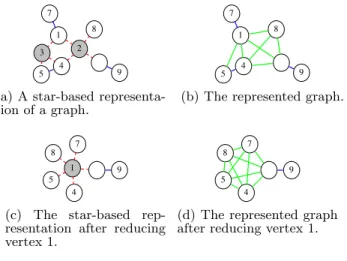
6 9 8 1 7
2 3
5 4
(a) A star-based representa-tion of a graph.
6 9 8 1 7
5 4
(b) The represented graph.
6 9
7 8
1 5
4
(c) The star-based rep-resentation after reducing vertex 1.
6 9
7 8
5 4
(d) The represented graph after reducing vertex 1.
Figure 1: Star-based representation and reduction. The white vertices are normal vertices, and gray ver-tices are hub verver-tices.
andcontractionof edges, which leads to improved scalability of several orders of magnitude.
Star-based Representation.
Here we deal with two kinds of graphs: A(star-based) representation graph is what we store and maintain in the memory, and arepresented graph corresponds to a virtual snapshot of a graph represented by a representation graph that would be maintained by the naive min-degree heuristic algorithm.In the star-based representation, each vertex belongs to one of the following two types: normal vertices orhub ver-tices. Two hub vertices are never connected, i.e., edges con-nect either two normal vertices or a normal vertex and a hub vertex. The represented graph can be obtained by a repre-sentation graph by(1) adding edges to make its neighbors a clique for all hub vertices and(2)removing hub vertices. For example, the representation graphs shown in Figures 1a and 1c represents the graphs shown in Figures 1b and 1d, respectively.
Overall Algorithm.
At a high level, our algorithm con-ducts the min-degree heuristic (Algorithm 3) on virtually represented graphs, i.e., it repeatedly reduces vertices with degree at mostdin the represented graph to generate a list of bags. Then our algorithm constructs the tree of the bags. To construct the tree, we use the same tree construction algorithm. Therefore, as noted before, the main difference here is that, during the reduction phase, we do not main-tain the represented graph itself. We manage the star-based representation graph instead. Thus, we explain how to re-duce vertices using star-based representation for enumerat-ing bags.Reducing a Vertex.
First, for a easier case, we consider a situation in which we reduce vertexv, whose neighbors are all normal vertices. To removev and make its neighbors a clique in the represented graph, we must alter the vertex type ofvfrom normal to hub.Let us now consider a general situation, where some of
v’s neighbors in the representation graph are hub vertices. One of the challenges here is the fact that no direct edges can exist in the representation graph between some of v’s neighbors due to these neighbor hub vertices. To makev’s
neighbors a clique in the represented graph, we must create a new hub vertex that is connected to all these neighbors.
Rather than creating such a new hub from scratch, the new hub can be efficiently composed by contracting v and all the neighboring hub vertices. Contraction of two ver-tices means removing the edge between them and merging two endpoints. For example, reducing the vertex 1 in the represented graph shown in Figure 1b corresponds to con-tracting vertices 1, 2, and 3 in the representation graph de-picted in Figure 1a, thus yielding the representation graph in Figure 1c. By doing so, as we will discuss in Section 5.2.2, the time complexity becomes almost linear to the output size using proper data structures. Moreover, we never add any new edge to the representation graph. Therefore, the number of edges in the representation graph never increases; thus, space consumption is also kept in linear.
5.2.2
Details
Finding a Vertex to Reduce: Precisely finding a vertex with minimum degree is too costly because we must track the degree of all vertices. Therefore, we approximately find a vertex with minimum degree by using a priority queue as follows. First, we insert all vertices into the priority queue, and use their current degree as keys. To find a vertex to reduce, we pop a vertex with the smallest key from the pri-ority queue. If its current degree is the same as the key, then we reduce the vertex. Otherwise, we reinsert the vertex to the priority queue with its new degree.
Data Structures: We manage adjacency lists in hash ta-bles to operate edges in constant time. To efficiently con-tract edges, we manage groups of vertices and merge adja-cency lists, similar to the weighted quick-find algorithm [46]. Core-tree-decomposition Ordering: For our total PPR algorithm, in addition to the decomposition, we also require ordering of verticesV(G)\Vr that satisfies the conditions
specified in Section 2.4. Actually, this can be obtained easily by the order of vertices to be reduced. It is easy to see that this ordering satisfies the conditions.
Time Complexity: As we contract vertices similar to the weighted quick-find algorithm, the expected total time con-sumed for edge contractions isO(m) time [30]. Reducing a vertexvtakes approximatelyO(d′), whered′is the degree of
v. Therefore, we expect that the proposed algorithm com-putes a core-tree-decomposition in P
i<didi+O(m) time,
wherediis the number of vertices of degreei. In Section 6.1,
we point outP
i<didi≤d/10×n. In particular, it runs in
linear time ifdis a constant.
6.
THEORETICAL ANALYSIS AND
EXPER-IMENTAL VERIFICATION
LetG= (Tr,V) be a rooted tree-decomposition of widthd
andVrcorresponding to the core. Here, we give a theoretical
analysis of our proposed algorithm. Then we justify it by performing several experiments.
We first show that our algorithm to construct an LU de-composition for a small tree-width part is very efficient. This can be qualified by giving an upper bound for fill-in (Section 6.1), which is also an upper bound for the time complexity to construct an LU decomposition. Our next empirical re-sults imply that the core Vr is very close to an expander
graph (Section 6.2). So far, we have examined undirected graphs.
In Sections 6.3 and 6.4, we show that a direct method works very well for small tree-width graphs; however a direct method does not work well for expander graphs. Moreover, an iterative method works very well for expander graphs, but does not for small tree-width graphs. These two facts would clarify theoretical hypothesis for our proposed algorithm. Thus, we need to look at directed graphs for this purpose. We also perform some experiments to support these facts.
6.1
How Many ”Fill-in”?
Here, we estimate an upper bound for the number of fill-in. As in Algorithm 1, our algorithm starts withv1and proceeds
in the order ofW. Let us considervi. The number of
fill-in forvi is exactly same as that of non-edges between any
nonadjacent vertices inNvi∩Wi, which is bounded by|Vt′|
2,
where the bagVt′ contains all the vertices ofN(vi)∩Wifor
some t′ ∈ T\ {r}. It follows that the number of fill-in is at most P
t∈T\{r}|Vt|2. By our construction of the
core-tree-decomposition, naively P
t∈T\{r}|Vt|2 is proportional
toP
i<di
2d
i, wheredi is the number of vertices of degreei
inV(G)\Vr. Note that we keep the small tree-width graph
even after adding edges. To estimateP
i<di
2d
i more accurately, we must look at
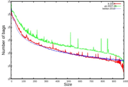
the distribution of the bag size of the core-tree-decompositions of the graphs shown in Figure 23. As is shown, many bags are small, and only a few bags are large. This can be ex-plained from a theoretical perspective. Ascale-free network is a network whose degree distribution follows a power law, at least asymptotically. That is, the fraction P(k) of ver-tices in the network having degree exactlykfor large values ofk can be described as follows:
P(k)∼ k−γ,
whereγis a parameter whose value is typically in the range 2 < γ < 3. Many networks are observed to be scale-free, including social networks and web graphs. Our core-tree-decomposition is based on minimum degree heuristic, which depends on degree distribution. Therefore, in prac-tice,P
i<didi≤
P
i<di×n/i
2≤d/10×nandP
i<di
2d
i≤
P
i<di
2×n/i2≤d×n.
101 102 103 104 105 106 107
0 100 200 300 400 500 600 700 800 900 1000
Number of bags
Size
it-2004 uk-2007-05 twitter-2010
Figure 2: Distribution of bag sizes.
6.2
How Close the Core is to Expander?
As explained previously, we determine how close the core of real networks is to expander by evaluating the distribu-tion of the eigenvalues of the transidistribu-tion matrix. For two synthetic networks (a typical expander graph and a typi-cal non-expander graph), two real web graphs (it-2004 and
3Datasets are explained in Section 7.
-1 -0.8 -0.6 -0.4 -0.2 0 0.2 0.4 0.6 0.8 1 -1
-0.8 -0.6 -0.4 -0.2 0 0.2 0.4 0.6 0.8 1
(a) Erd˝os-R´enyi ran-dom graph
-1 -0.8 -0.6 -0.4 -0.2 0 0.2 0.4 0.6 0.8 1 -1
-0.8 -0.6 -0.4 -0.2 0 0.2 0.4 0.6 0.8 1
(b) Binary tree with random edges added
-1 -0.8 -0.6 -0.4 -0.2 0 0.2 0.4 0.6 0.8 1 -1
-0.8 -0.6 -0.4 -0.2 0 0.2 0.4 0.6 0.8 1
(c) it-2004
-1 -0.8 -0.6 -0.4 -0.2 0 0.2 0.4 0.6 0.8 1 -1
-0.8 -0.6 -0.4 -0.2 0 0.2 0.4 0.6 0.8 1
(d) uk-2007-05
-1 -0.8 -0.6 -0.4 -0.2 0 0.2 0.4 0.6 0.8 1 -1
-0.8 -0.6 -0.4 -0.2 0 0.2 0.4 0.6 0.8 1
(e) twitter-2010
-1 -0.8 -0.6 -0.4 -0.2 0 0.2 0.4 0.6 0.8 1 -1
-0.8 -0.6 -0.4 -0.2 0 0.2 0.4 0.6 0.8 1
(f) livejournal
Figure 3: Extreme eigenvalues of typical networks on complex plane; x axis is for the real part and
y axis is for the imaginary part. Red points are the distribution of eigenvalues of the whole network, purple points are that of the core with d= 10, blue points are that of the core with d= 100, and green points are that of the core with d = 1000. For (a) and (b), there are only red and blue points.
uk-2007-05), and two real social networks (twitter-2010 and livejournal)4, we compute 200 extreme eigenvalues of the
transition matrix of their cores and their whole networks, respectively, using the Arnoldi method [40]. The results are shown in Figure 3. The transition matrices are not neces-sarily symmetric; thus, eigenvalues may not be real. In fact, they contain both the real part and the imaginary part, as shown in Figure 3.
Figure 3a indicates a directed version of an Erd¨os-R´enyi random graph, which is supposed to be a typical expander graph, and Figure 3b indicates a directed complete binary tree with a few random edges added, which is a typical non-expander graph (i.e., a small tree-width graph). As explained previously, a given network is close to expander if the eigenvalues are clustered near the origin. This can be also qualified by Figures 3a and 3b.
For real networks (Figures 3c–3f), the eigenvalues of the whole networks (red points) are scattered, similar to the dis-tribution of a non-expander graph (Figure 3b). On the other hand, the eigenvalues of the core (blue points) are relatively
clustered near the origin, similar to the distribution of an expander graph (Figure 3a). These results suggest that
real networks are non-expanders but the core of each network is closer to an expander.
6.3
Direct Method Is Fast on Small Tree-Width
Graphs
From the analysis in Section 6.1, if a graph is of tree-width
dthen the number of fill-in isO(nd). Thus, the number of nonzero elements inL and U is O(m+nd). Therefore, if the tree-width of a given graph is larger, then it is expected to take much more time to find an LU decomposition.
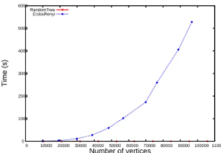
We now verify this discussion for real networks by finding an LU decomposition for typical synthetic undirected net-works (i.e., Erd˝os-R´enyi and binary tree with random edges added). The tree-width of an Erd˝os-R´enyi random graph is
O(n) [24], and the tree-width of a binary-tree isO(1). Both graphs have m = O(n) edges; however the computational time required to find an LU decomposition (and hence for a direct method) is quite different (Figure 4). This coincides with the above theoretical observation.
0 1000 2000 3000 4000 5000 6000
0 10000 20000 30000 40000 50000 60000 70000 80000 90000 100000 110000
Time (s)
Number of vertices RandomTree
ErdosRenyi
Figure 4: Computational time of LU decomposition. Note that in the literature for a sparse direct method, many re-ordering methods are proposed to reduce the num-ber of fill-ins [5, 25]; however if a graph has a large tree-width, any ordering cannot reduce the computational cost, as shown in Figure 4. Therefore, we conclude that decom-posing a graph into the small tree-width part and thecore part is more important than finding a better ordering.
6.4
Iterative Method Is Fast on Expander
Graphs
Here, we show that iterative methods, in particular GM-RES, converge quickly if a network is close to expander.
Let us start with the analysis of the Power iteration. The Power iteration for PPR is given by
x(t+1)=αP x(t)+ (1−α)b.
To simplify the following discussion, we assumex(0)= (1−
α)b. By substituting the left side to the right side iteratively, we obtain
x(t)= (1−α)
I+αP+· · ·+αt−1Pt−1
b
and hence the residualr(t)= (1−α)b−(I−αP)x(t)satisfies
kr(t)k ≤αtkPtr(0)k. (4) The standard analysis of PPR uses this formula and applies the Perron-Frobenius theorem to show that the convergence
rate isO(αt) [38]. However, we should take advantage of an expander graph; thus more detailed analysis is required.
Suppose that the transition matrixP is diagonalizable, i.e., U−1P U = diag(λ1, . . . , λn) for an eigenvector matrix U = [v1. . . vn]. Without loss of generality, we may assume
that 1 = λ1 ≥ |λ2| ≥ · · · ≥ |λn|. Then, by expanding r(0)= (1−α)bby the eigenvectors ofP as
r(0)=β1u1+· · ·+βnun, (5)
and substituting to (4), we obtain kr(t)k ≤αt
n
X
i=1
|λi|t|βi|. (6)
As explained before in the case of an expander graph, the second eigenvalue of an expander graph is relatively small compared to the first eigenvalue [14]. Therefore, all terms except for the first converge rapidly; thus the Power itera-tion converges quickly. However, this does not give us im-provement. The asymptotic convergence rate of the Power iteration is stillO(αt) because the first eigenvector
compo-nent is a bottleneck.
To take the advantage of expander, we have a closer look at the GMRES algorithm. We consider Embree [19]’s re-sult, which is a generalization of (6). Here, let κi be the
condition number of i’th eigenvalue λi, which is defined as κi = kuLikkuRik/|u∗LiuRi|, where uLi and uRi are the left
and right eigenvectors ofλi, respectively. Then, forany
poly-nomial p(z) of degreetandp(0) = 1, we have the following bound [19]:
kr(t)k ≤
n
X
i=1
|p(1−αλi)|κi. (7)
Generally, we do not know the optimal polynomialpto min-imize the right side of (7) which gives tight convergence es-timation. However, by using some explicit polynomialp, we can obtain an upper bound of convergence estimation.
Let us first use a simple polynomialp(z) = (1−z)t. Thus
(7) gives
kr(t)k ≤αt n
X
i=1
|λi|tκi,
which is a similar form of (6). This implies that GMRES requires at most the same number of iterations of Power iter-ation. To take further advantage of the expander property, let us usep(z)∝(1−α−z)(1−z)t−1. Then, (7) gives
kr(t)k ≤Kαt n
X
i=2
|λi|tκi
for some constant K. We emphasize that the summation starts fromi= 2, i.e., the term fori= 1 is removed. This shows that GMRES can remove the effect of the first eigen-vector component, which is the bottleneck of the Power it-eration. Thus the convergence rate of GMRES is at least
O(|αλ2|t). This significantly improves the Power iteration
when a given graph is an expander, i.e.,|λ2| ≪1.
We verify the above discussion empirically by applying Power iteration and GMRES to typical synthetic networks. Consider an Erd˝os-R´enyi random graph and a binary tree with random edges, whish are typical expander and non-expander graphs, respectively. We plot the error curves of
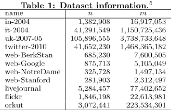
Table 1: Dataset information.5
name n m
in-2004 1,382,908 16,917,053 it-2004 41,291,549 1,150,725,436 uk-2007-05 105,896,555 3,738,733,648 twitter-2010 41,652,230 1,468,365,182 web-BerkStan 685,230 7,600,505 web-Google 875,713 5,105,049 web-NotreDame 325,728 1,497,134 web-Stanford 281,903 2,312,497 livejournal 5,284,457 77,402,652 flickr 1,846,198 22,613,981 orkut 3,072,441 223,534,301
the Power iteration and GMRES for these networks in Fig-ure 5. Observe that the error curve for an expander graph is shown in Figure 5a. Both the Power iteration and GMRES have a steeper slope in the first few iterations. However, in the latter iterations, the slope of GMRES stays steep, but the slope of the Power iteration becomes gentle. This result implies that
iterative methods are fast for expander graphs. In particular, GMRES can exploit much more information on expander graphs than the Power iteration.
Next, we examine the error curves for non-expander graphs. The results are shown in Figure 5b. We can see that the error curves of the Power iteration and GMRES are com-pletely overlapped, because, as there are too many larger eigenvalues, there is no good polynomialp that shows the rapid convergence of GMRES. Since the computational cost of a single iteration of GMRES is more expensive than that of the Power iteration [18, 26], we can conclude that
GMRES cannot outperform the Power iteration for non-expander graphs.
10-7
10-6 10-5
10-4
10-3 10-2 10-1
100
0 10 20 30 40 50 60 70 80 90
Accuracy
Number of iterations Power GMRES
(a) Erd˝os-R´enyi random graph 10-7
10-6 10-5
10-4
10-3 10-2 10-1
100
0 10 20 30 40 50 60 70 80 90
Accuracy
Number of iterations Power GMRES
(b) Binary tree with random edges
Figure 5: Comparison between the Power iteration and GMRES.
7.
EXPERIMENTAL EVALUATION
We conducted experiments on several web graphs as well as a few social networks. The purpose of the experiments is to demonstrate performance of our proposed algorithm for both the preprocessing and the computation for PPR.
All experiments are conducted on an Intel Xeon E5-2690 2.90GHz CPU with 256GB memory and running Ubuntu 12.04. Our algorithm is implemented in C++ and compiled with g++v4.6 with -O3 option. We use 10 directed and 1 undirected (orkut) networks shown in Table 1.
5in-2004, it-2004, uk-2007-05, and twitter-2010 data sets are
available at http://law.di.unimi.it/datasets.php [11,
Table 2: Preprocessing; widthd= 100. name CT dec[s] core size LU dec[s] in-2004 0.39 41,475 1.41 it-2004 162.90 4,309,140 43.45 uk-2007-05 528.26 13,009,914 101.47 twitter-2010 197.32 7,513,858 16.81 web-BerkStan 2.02 36,823 0.83 web-Google 2.22 41,693 0.83 web-NotreDame 0.42 5,252 0.31 web-Stanford 0.70 10,393 0.35 livejournal 33.81 1,174,081 3.74 flickr 12.91 148,385 0.88 orkut 28.53 1,950,126 1.13
Preprocessing.
The experimental results for the prepro-cessing phase are shown in Table 2. For these networks we set the width dof the core-tree-decomposition asd = 100. We also perform the preprocessing phase with varying d. The results will be given later; however,d= 100 is the aver-age case (i.e., CT+LU in Table 2) for many datasets. Thus let us fixd= 100 for the moment. We perform our algorithm 100 times and take the average.For these networks, the computational time to construct a core-tree-decomposition (CT in Table 2) and an LU de-composition (LU in Table 2) is essentially proportional to the number of vertices and edges. However it varies signifi-cantly among the networks. The size of the core also varies among the networks
These experiments show that we can perform our prepro-cessing very quickly to obtain both a core-tree-decomposition and an LU decomposition of the small tree-width part.
Personalized PageRank computation and comparison
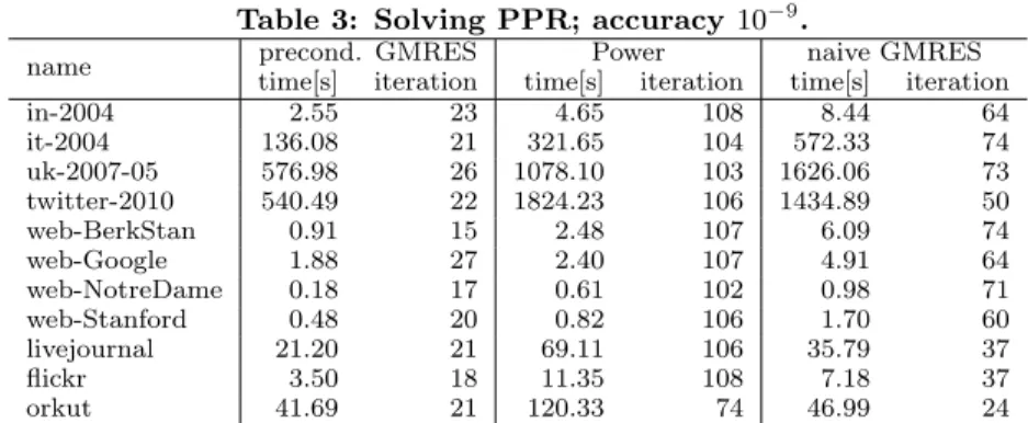
to other algorithms.
The experimental results for the PPR computation phase are shown in Table 3. We take the per-sonalized vectorbsuch that the number of nonzero elements is four, and these nonzero elements are randomly chosen6 All algorithms in Table 3 must computex∈Rn such that kx−x∗k ≤10−9kx∗k, wherex∗∈Rnis a vector of the op-timal PPR (accuracy 10−9in Table 3). We setα= 0.85, as it is widely used. We perform our algorithm 100 times and take the average.
We compare our algorithm with the Power method and the naive GMRES method [44](Note that no preconditioning is performed).
First, let us look at our algorithm, the preconditioned GMRES, and the Power method, and the naive GMRES method. The proposed algorithm is 2–5 times faster than the Power method and 1.5–6 times faster than the naive GMRES method. Even if we consider the preprocessing time into account for the query time, our proposed algorithm is 2-4 times faster than the Power method and the naive GMRES method. Note that the number of iterations of our algorithm is very small, say 5 times less than the Power method. These results suggest that if we handle millions of query requests simultaneously, then once we have performed one efficient preprocessing for a large network (e.g., once a 12]. BerkStan Google, NotreDame, and web-Stanford data sets are available athttp://snap.stanford. edu/data/index.html [3, 33]. livejournal, flickr, and orkut data sets are available at http://socialnetworks. mpi-sws.org/datasets.html[37].
6In word sense disambiguation, the number of query nodes
Table 3: Solving PPR; accuracy10−9.
name precond. GMRES Power naive GMRES time[s] iteration time[s] iteration time[s] iteration in-2004 2.55 23 4.65 108 8.44 64 it-2004 136.08 21 321.65 104 572.33 74 uk-2007-05 576.98 26 1078.10 103 1626.06 73 twitter-2010 540.49 22 1824.23 106 1434.89 50 web-BerkStan 0.91 15 2.48 107 6.09 74 web-Google 1.88 27 2.40 107 4.91 64 web-NotreDame 0.18 17 0.61 102 0.98 71 web-Stanford 0.48 20 0.82 106 1.70 60 livejournal 21.20 21 69.11 106 35.79 37 flickr 3.50 18 11.35 108 7.18 37 orkut 41.69 21 120.33 74 46.99 24
Table 4: Computational time for various bag sizes
d. PPR column shows the number of iterations in parenthesis.
it-2004 twitter-2010
d CT[s] LU[s] PPR[s] CT[s] LU[s] PPR[s]
10 8.87 10.48 148.44(26) 17.77 14.06 540.78(23) 20 24.58 14.71 142.79(25) 39.05 15.61 547.89(23) 50 78.94 26.60 134.35(23) 107.73 15.35 589.16(23) 100 162.90 43.45 136.08(21) 197.32 16.81 540.49(22) 200 276.96 70.86 148.40(21) 353.61 19.74 547.51(22) 500 476.99 219.24 160.97(20) 958.65 21.67 577.86(22) 1000 690.73 563.77 168.15(19) 2265.78 21.53 557.14(22) day because the network may change in a single day), our algorithm can handle millions of query requests up to five times more efficiently than the Power method and the naive GMRES method.
Bag size and computational time.
As mentioned above,d = 100 is the average case for many datasets; however, sometimes our algorithm runs faster if d is smaller. This is the case for a web graph (it-2004) and a social network (twitter-2010). The results are shown in Table 4. For these two datasets, the time for PPR (i.e., our proposed query phase) does not vary significantly. Therefore, we can obtain a slightly faster algorithm (for CT + LU + PPR).
Here we present theoretical justification. First, Let us look at Figures 3c and 3d for web graphs and Figures 3e and 3f for social networks. We compute 200 “extreme” eigenvalues of the whole networks and of only their cores for the cases
d = 10, 100, and 1000, respectively, by using the Arnoldi method [40]. We can conclude that asdincreases, the eigen-values of the cores of web graphs are clustered closer to the origin. This means that as d increases, the core of web graphs gets closer to an expander (similar to the distribu-tion of an expander graph (Figure 3a)). On the other hand, asdincreases, the eigenvalues of the cores of social networks are first clustered closer to the origin, but then stay for a while. This means that, for social networks, we can stop at some value ofd. Indeed,d= 100 seems sufficient for social networks.; however for web graphs, we can increased.
8.
RELATED WORK
We discuss previous work related to PPR computation. Several approximate approaches have been proposed fo-cusing on efficient computation for PPR. However, none of them seems to guarantee an accurate solution. Their out-puts differ from those of iterative methods. Therefore, it is
difficult for these approximate approaches to compare the quality of real applications with ours.
Having said that, Jeh and Widom have suggested a frame-work that provides a scalable solution for PPR for vertices that belong to a highly linked subset of hub vertices [28]. Their approach is based on the observation that relevance scores for a given distribution can be approximated as a linear combination of those from a single vertex in hubs. They compute approximate relevance scores for a given dis-tribution using relevance scores that can be precomputed from hubs. Fogaras et al. [21] proposed a Monte Carlo based algorithm for PPR. To compute approximate rele-vance scores, they used fingerprints of several vertices; a fingerprint of a vertex is a random walk starting from the vertex. They first preprocess fingerprints by simulating ran-dom walks, and then approximate relevance distributions from the ending vertices of these random walks. They ap-proximated relevance scores by exploiting the linearity prop-erty of PPR. Avrachenkov et al. [7] and Bahmani, Chowd-hury, and Goel [8], independently, improved the Monte Carlo method.
9.
CONCLUSION
In this paper, by exploiting graph structures of web graphs and social networks, we have proposed a GMRES (a state-of-the-arts advanced iterative method) based algorithm to compute the personalized PageRank for web graphs and so-cial networks. The convergence of the algorithm is very fast. In fact, it is as much as 7.5 times less than the Power method for the number of iterations and as much as five times faster than the Power method in actual computation time. Even if we consider the preprocessing time into account for the query time, the proposed algorithm is 2-4 times faster than the Power method. In addition, we can implement our al-gorithm for graphs with billions of edges. If we must handle millions of query requests simultaneously, then once we have performed a single efficient preprocessing for a large network (once a day because the network may change in a single day), our algorithm can handle millions of query requests up to five times more efficiently.
Finally, we would mention that our experimental results imply that web graphs and social networks are different in the structure of core-tree-decomposition. In [1], we extend this idea and analyze several real networks via core-tree-decomposition.
Acknowledgment
The second author is supported by a Grant-in-Aid for JSPS Fellows (256563). The third author is supported by a Grant-in-Aid for JSPS Fellows (256487).
10.
REFERENCES
[1] T. Akiba, T. Maehara, and K. Kawarabayashi. Network structural analysis via core-tree-decomposition. InKDD, 2014, to appear.
[2] T. Akiba, C. Sommer, and K. Kawarabayashi.
Shortest-path queries for complex networks: exploiting low tree-width outside the core. InEDBT, pages 144–155, 2012. [3] R. Albert, H. Jeong, and A.-L. Barabasi. Diameter of the
World-Wide Web.Nature, 1999.
[4] N. Alon and F. R. Chung. Explicit construction of linear sized tolerant networks.Ann. Disc. Math., 38:15–19, 1988. [5] P. R. Amestoy, T. A. Davis, and I. S. Duff. An approximate
minimum degree ordering algorithm.SIMAX, 17:886–905, 1996.
[6] S. Arnborg and A. Proskurowski. Linear time algorithms for NP-hard problems restricted to partialk-trees.Disc. Appl. Math., 2:11–24, 1989.
[7] K. Avrachenkov, N. Litvak, D. Nemirovsky, E. Smirnova, and M. Sokol. Quick detection of top-k personalized PageRank lists. InWAW, pages 50–61, 2011.
[8] B. Bahmani, A. Chowdhury, and A. Goel. Fast incremental and personalized PageRank. InPVLDB, volume 4, pages 173–184, 2010.
[9] S. M. Beitzel, E. C. Jensen, A. Chowdhury, D. Grossman, and O. Frieder. Hourly analysis of a very large topically categorized web query log. InSIGIR, pages 321–328, 2004. [10] A. Berry, P. Heggernes, and G. Simonet. The minimum
degree heuristic and the minimal triangulation process. In
Graph-Theoretic Concepts in Computer Science, volume 2880, pages 58–70. 2003.
[11] P. Boldi, M. Rosa, M. Santini, and S. Vigna. Layered label propagation: A multiresolution coordinate-free ordering for compressing social networks. InWWW, 2011.
[12] P. Boldi and S. Vigna. The WebGraph framework I: Compression techniques. InWWW, pages 595–601, 2004. [13] R. Chen, X. Weng, B. He, and M. Yang. Large graph
processing in the cloud. InSIGMOD, pages 1123–1126, 2010.
[14] F. Chung.Spectral Graph Theory. Cbms Regional Conference Series in Mathematics, 1997.
[15] F. Chung. Laplacians and the Cheeger inequality for directed graphs.Ann. Comb., 9(1):1–19, 2005. [16] T. A. Davis.Direct methods for sparse linear systems.
SIAM, 2006.
[17] J. Dean and S. Ghemawat. MapReduce: simplified data processing on large clusters. InOSDI, pages 10–10, 2004. [18] G. M. Del Corso, A. Gull´ı, and F. Romani. Comparison of
Krylov subspace methods on the PageRank problem.J. Comput. Appli. Math., 210:159–166, 2007.
[19] M. Embree. How descriptive are GMRES convergence bounds? Technical report, Oxford University Computing Laboratory, 1999.
[20] Facebook. http://facebook.com/press/info.php?statistics, 2012.
[21] D. Fogaras, B. R´acz, K. Csalog´any, and T. Sarl´os. Towards scaling fully personalized PageRank: Algorithms, lower bounds, and experiments.Internet Math., 2, 2005. [22] Y. Fujiwara, M. Nakatsuji, M. Onizuka, and
M. Kitsuregawa. Fast and exact top-k search for random walk with restart. InPVLDB, volume 5, pages 442–453, 2012.
[23] Y. Fujiwara, M. Nakatsuji, T. Yamamuro, H. Shiokawa, and M. Onizuka. Efficient personalized PageRank with accuracy assurance. InKDD, pages 15–23, 2012.
[24] Y. Gao. Treewidth of Erd˝os–R´enyi random graphs, random intersection graphs, and scale-free random graphs.Disc. Appl. Math., 160:566–578, 2012.
[25] A. George. Nested dissection of a regular finite element mesh.SINUM, 10:345–363, 1973.
[26] D. Gleich, L. Zhukov, and P. Berkhin. Fast parallel PageRank: A linear system approach.Yahoo! Research Technical Report YRL-2004-038, 13:22, 2004.
[27] S. Hoory, N. Linial, and A. Wigderson. Expander graphs and their applications.Bull. Amer. Math. Soc.,
43(4):439–561, 2006.
[28] G. Jeh and J. Widom. Scaling personalized web search.
WWW, pages 271–279, 2003.
[29] M. Jerrum and A. Sinclair. Approximating the permanent.
SIAM J. Comput., 18(6):1149–1178, 1989.
[30] D. E. Knuth and A. Sch¨onhage. The expected linearity of a simple equivalence algorithm.Theor. Comput. Sci., 6:281–315, 1978.
[31] H. Kwak, C. Lee, H. Park, and S. Moon. What is twitter, a social network or a news media?WWW, 2010.
[32] A. N. Langville and C. D. Meyer.Google’s PageRank and beyond: The science of search engine rankings. Princeton University Press, 2006.
[33] J. Leskovec, K. Lang, A. Dasgupta, and M. Mahoney. Community structure in large networks: Natural cluster sizes and the absence of large well-defined clusters.Internet Math., 6:29–123, 2009.
[34] D. Liben-Nowell and J. Kleinberg. The link prediction problem problem for social networks. InCIKM, pages 556–559, 2003.
[35] Y. Low, J. Gonzalez, A. Kyrola, D. Bickson, C. Guestrin, and J. M. Hellerstein. Distributed GraphLab: A framework for machine learning and data mining in the cloud. In
PVLDB, volume 5, pages 716–727, 2012.
[36] G. Malewicz, M. H. Austern, A. J. Bik, J. Dehnert, I. Horn, N. Leiser, , and G. Czajkowski. Pregel: a system for large-scale graph processing. pages 135–146, 2010. [37] A. Mislove, M. Marcon, K. P. Gummadi, P. Druschel, and
B. Bhattacharjee. Measurement and analysis of online social networks. InIMC, pages 29–42, 2007.
[38] L. Page, S. Brin, R. Motwani, and T. Winograd. The pagerank citation ranking: Bringing order to the web. Technical report, Stanford InfoLab, 1999.
[39] N. Robertson and P. D. Seymour. Graph minors. III. planar tree-width.J. Combin. Theory Ser. B, 36:49–63, 1984. [40] Y. Saad.Numerical methods for large eigenvalue problems,
volume 158. SIAM, 1992.
[41] Y. Saad.Iterative methods for sparse linear systems. SIAM, 2003.
[42] Y. Saad and M. H. Schultz. GMRES: a generalized minimal residual algorithm for solving nonsymmetric linear systems.
SISSC, 7:869–869, 1986.
[43] F. Wei. Tedi: efficient shortest path query answering on graphs. InSIGMOD, pages 99–110, 2010.
[44] G. Wu and Y. Wei. Arnoldi versus GMRES for computing PageRank: A theoretical contribution to Google’s PageRank problem.ACM Trans. Inf. Syst., 28(3):11:1–11:28, 2010.
[45] J. Xu, F. Jiao, and B. Berger. A tree-decomposition approach to protein structure prediction. InCSB, pages 247–256, 2005.
[46] A. C.-C. Yao. On the average behavior of set merging algorithms. InSTOC, pages 192–195, 1976.