March 1999
More
Than You Ever Wanted To Know
*
About
Volatility Swaps
Kresimir Demeterfi
Emanuel Derman
Michael Kamal
Joseph Zou
Copyright 1999 Goldman, Sachs & Co. All rights reserved.
This material is for your private information, and we are not soliciting any action based upon it. This report is not to be construed as an offer to sell or the solicitation of an offer to buy any security in any jurisdiction where such an offer or solicitation would be illegal. Certain transactions, including those involving futures, options and high yield securities, give rise to substantial risk and are not suitable for all investors. Opinions expressed are our present opinions only. The material is based upon information that we consider reliable, but we do not represent that it is accurate or complete, and it should not be relied upon as such. We, our affiliates, or persons involved in the preparation or issuance of this material, may from time to time have long or short positions and buy or sell securities, futures or options identical with or related to those mentioned herein.
This material has been issued by Goldman, Sachs & Co. and/or one of its affiliates and has been approved by Goldman Sachs International, regulated by The Securities and Futures Authority, in connection with its distribution in the United Kingdom and by Goldman Sachs Canada in connection with its distribution in Canada. This material is distributed in Hong Kong by Goldman Sachs (Asia) L.L.C., and in Japan by Goldman Sachs (Japan) Ltd. This material is not for distribution to private customers, as defined by the rules of The Securities and Futures Authority in the United Kingdom, and any investments including any convertible bonds or derivatives mentioned in this material will not be made available by us to any such private customer. Neither Goldman, Sachs & Co. nor its representative in Seoul, Korea is licensed to engage in securities business in the Republic of Korea. Goldman Sachs International or its affiliates may have acted upon or used this research prior to or immediately following its publication. Foreign currency denominated securities are subject to fluctuations in exchange rates that could have an adverse effect on the value or price of or income derived from the investment. Further information on any of the securities mentioned in this material may be obtained upon request and for this purpose persons in Italy should contact Goldman Sachs S.I.M. S.p.A. in Milan, or at its London branch office at 133 Fleet Street, and persons in Hong Kong should contact Goldman Sachs Asia L.L.C. at 3 Garden Road. Unless governing law permits otherwise, you must contact a Goldman Sachs entity in your home jurisdiction if you want to use our services in effecting a transaction in the securities mentioned in this material.
Note: Options are not suitable for all investors. Please ensure that you have read and understood the current options disclosure document before entering into any options transactions.
SUMMARY
Volatility swaps are forward contracts on future realized stock volatility. Variance swaps are similar contracts on vari-ance, the square of future volatility. Both of these instruments provide an easy way for investors to gain exposure to the future level of volatility.
Unlike a stock option, whose volatility exposure is contami-nated by its stock-price dependence, these swaps provide pure exposure to volatility alone. You can use these instruments to speculate on future volatility levels, to trade the spread between realized and implied volatility, or to hedge the vola-tility exposure of other positions or businesses.
In this report we explain the properties and the theory of both variance and volatility swaps, first from an intuitive point of view and then more rigorously. The theory of variance swaps is more straightforward. We show how a variance swap can be theoretically replicated by a hedged portfolio of standard options with suitably chosen strikes, as long as stock prices evolve without jumps. The fair value of the variance swap is the cost of the replicating portfolio. We derive analytic formu-las for theoretical fair value in the presence of realistic vola-tility skews. These formulas can be used to estimate swap values quickly as the skew changes.
We then examine the modifications to these theoretical results when reality intrudes, for example when some neces-sary strikes are unavailable, or when stock prices undergo jumps. Finally, we briefly return to volatility swaps, and show that they can be replicated by dynamically trading the more straightforward variance swap. As a result, the value of the volatility swap depends on the volatility of volatility itself. _________________
Kresimir Demeterfi (212) 357-4611 Emanuel Derman (212) 902-0129 Michael Kamal (212) 357-3722
Joseph Zou (212) 902-9794
_________________
Acknowledgments: We thank Emmanuel Boussard,
Llewel-lyn Connolly, Rustom Khandalavala, Cyrus Pirasteh, David Rogers, Emmanuel Roman, Peter Selman, Richard Sussman, Nicholas Warren and several of our clients for many discus-sions and insightful questions about volatility swaps.
_________________ Editorial: Barbara Dunn
Volatility Swaps ... 1
Who Can Use Volatility Swaps? ... 2
Variance Swaps ... 3
Outline ... 4
I. REPLICATINGVARIANCESWAPS: FIRSTSTEPS... 6
The Intuitive Approach ... 6
Trading Realized Volatility with a Log Contract ... 11
The Vega, Gamma and Theta of a Log Contract ... 11
Imperfect Hedges ... 13
The Limitations of the Intuitive Approach ... 13
II. REPLICATINGVARIANCESWAPS: GENERALRESULTS... 15
Valuing and Pricing the Variance Swap... 17
III. ANEXAMPLE OF AVARIANCESWAP ... 20
IV. EFFECTS OF THEVOLATILITYSKEW ... 23
Skew Linear in Strike ... 23
Skew Linear in Delta ... 25
V. PRACTICALPROBLEMS WITHREPLICATION ... 27
Imperfect Replication Due to Limited Strike Range ... 27
The Effect of Jumps on a Perfectly Replicated Log Contract .. 29
The Effect of Jumps When Replicating With a Finite Strike Range... 32
VI. FROMVARIANCE TOVOLATILITYCONTRACTS ... 33
Dynamic Replication of a Volatility Swap ... 34
CONCLUSIONS ANDFUTUREINNOVATIONS ... 36
APPENDIXA: REPLICATINGLOGARITHMICPAYOFFS... 37
APPENDIXB: SKEWLINEAR INSTRIKE... 40
APPENDIXC: SKEWLINEAR INDELTA... 44
APPENDIXD: STATIC ANDDYNAMICREPLICATION OF A VOLATILITYSWAP ... 48
INTRODUCTION A stock’s volatility is the simplest measure of its riskiness or uncer-tainty. Formally, the volatilityσRis the annualized standard deviation of the stock’s returns during the period of interest, where the subscript R denotes the observed or “realized” volatility. This note is concerned with volatility swaps and other instruments suitable for trading vola-tility1.
Why trade volatility? Just as stock investors think they know some-thing about the direction of the stock market, or bond investors think they can foresee the probable direction of interest rates, so you may think you have insight into the level of future volatility. If you think current volatility is low, for the right price you might want to take a position that profits if volatility increases.
Investors who want to obtain pure exposure to the direction of a stock price can buy or sell short the stock. What do you do if you simply want exposure to a stock’s volatility?
Stock options are impure: they provide exposure to both the direction of the stock price and its volatility. If you hedge the options according to Black-Scholes prescription, you can remove the exposure to the stock price. But delta-hedging is at best inaccurate because the real world violates many of the Black-Scholes assumptions: volatility cannot be accurately estimated, stocks cannot be traded continuously, transac-tions costs cannot be ignored, markets sometimes move discontinu-ously and liquidity is often a problem. Nevertheless, imperfect as they are, until recently options were the only volatility vehicle available.
Volatility Swaps The easy way to trade volatility is to use volatility swaps, sometimes called realized volatility forward contracts, because they provide pure exposure to volatility (and only to volatility).
A stock volatility swap is a forward contract on annualized volatility. Its payoff at expiration is equal to
(EQ 1)
whereσRis the realized stock volatility (quoted in annual terms) over the life of the contract, Kvol is the annualized volatility delivery price, and N is the notional amount of the swap in dollars per annualized vol-atility point. The holder of a volvol-atility swap at expiration receives N dollars for every point by which the stock’s realized volatility σRhas
1. For a discussion of volatility as an asset class, see Derman, Kamal, Kani, McClure, Pirasteh, and Zou (1996).
σR–Kvol
exceeded the volatility delivery price Kvol. He or she is swapping a fixed volatility Kvolfor the actual (“floating”) future volatilityσR.
The delivery price Kvolis typically quoted as a volatility, for example 30%. The notional amount is typically quoted in dollars per volatility point, for example, N = $250,000/(volatility point). As with all forward contracts or swaps, the fair value of volatility at any time is the deliv-ery price that makes the swap currently have zero value.
The procedure for calculating the realized volatility should be clearly specified with respect to the following aspects:
• The source and observation frequency of stock or index prices – for example, using daily closing prices of the S&P 500 index;
• The annualization factor in moving from daily or hourly observa-tions to annualized volatilities – for example, using 260 business days per year as a multiplicative factor in computing annualized variances from daily returns; and
• Whether the standard deviation of returns is calculated by subtract-ing the sample mean from each return, or by assumsubtract-ing a zero mean. The zero mean method is theoretically preferable, because it corre-sponds most closely to the contract that can be replicated by options portfolios. For frequently observed prices, the difference is usually negligible.
Who Can Use Volatility Swaps?
Volatility has several characteristics that make trading attractive. It is likely to grow when uncertainty and risk increase. As with interest rates, volatilities appear to revert to the mean; high volatilities will eventually decrease, low ones will likely rise. Finally, volatility is often negatively correlated with stock or index level, and tends to stay high after large downward moves in the market. Given these tendencies, several uses for volatility swaps follow.
Directional Trading of Volatility Levels. Clients who want to
spec-ulate on the future levels of stock or index volatility can go long or short realized volatility with a swap. This provides a much more direct method than trading and hedging options. For example, if you foresee a rapid decline in political and financial turmoil after a forthcoming elec-tion, a short position in volatility might be appropriate.
Trading the Spread between Realized and Implied Volatility Levels. As we will show later, the fair delivery price Kvolof a volatility swap is a value close to the level of current implied volatilities for options with the same expiration as the swap. Therefore, by unwinding
the swap before expiration, you can trade the spread between realized and implied volatility.
Hedging Implicit Volatility Exposure. There are several busi-nesses that are implicitly short volatility:
• Risk arbitrageurs or hedge funds often take positions which assume that the spread between stocks of companies planning mergers will narrow. If overall market volatility increases, the merger may become less likely and the spread may widen.
• Investors following active benchmarking strategies may require more frequent rebalancing and greater transactions expenses dur-ing volatile periods.
• Portfolio managers who are judged against a benchmark have track-ing error that may increase in periods of higher volatility.
• Equity funds are probably short volatility because of the negative correlation between index level and volatility. As global equity corre-lations have increased, diversification across countries has become a less effective portfolio hedge. Since volatility is one of the few parameters that tends to increase during global equity declines, a long volatility hedge may be appropriate, especially for financial businesses.
Variance Swaps Although options market participants talk of volatility, it is variance, or volatility squared, that has more fundamental theoretical signifi-cance. This is so because the correct way to value a swap is to value the portfolio that replicates it, and the swap that can be replicated most reliably (by portfolios of options of varying strikes, as we show later) is a variance swap.
A variance swap is a forward contract on annualized variance, the square of the realized volatility. Its payoff at expiration is equal to
(EQ 2)
where is the realized stock variance (quoted in annual terms) over the life of the contract, Kvaris the delivery price for variance, and N is the notional amount of the swap in dollars per annualized volatility point squared. The holder of a variance swap at expiration receives N dollars for every point by which the stock’s realized variance has exceeded the variance delivery price Kvar.
σR2
Kvar
–
( )×N
σ2R
Though theoretically simpler, variance swaps are less commonly traded, and so their quoting conventions vary. The delivery price Kvar can be quoted as a volatility squared, for example (30%)2. Similarly, for example, the notional amount can be expressed as $100,000/(one vola-tility point)2. The fair value of variance is the delivery price that makes the swap have zero value.
Outline Most of this note will focus on the theory and properties of variance swaps, which provide similar volatility exposure to straight volatility swaps. Because of its fundamental role, variance can serve as the basic building block for constructing other volatility-dependent instruments. At the end, we will return to a discussion of the additional risks involved in replicating and valuing volatility swaps.
Section I presents an intuitive, Black-Scholes-based account of the fun-damental strategy by which a variance swap can be replicated and val-ued. First, we show that the hedging of a (slightly) exotic stock option, the log contract, provides a payoff equal to the variance of the stock’s returns under a fairly wide set of circumstances. Then, we explain how this exotic option itself can be replicated by a portfolio of standard stock options with a range of strikes, so that their market prices deter-mine the cost of the variance swap. We also provide insight into the swap by showing, from a variety of viewpoints, how the apparently complex hedged log contract produces an instrument with the simple constant exposure to the realized variance of a variance swap.
Section II derives the same results much more rigorously and gener-ally, without depending on the full validity of the Black-Scholes model. Though more difficult, this presentation is capable of much greater generalization.
In Section III, we provide a detailed numerical example of the valua-tion of a variance swap. Some practical issues concerning the choice of strikes are also discussed.
The fair value of the variance swap is determined by the cost of the replicating portfolio of options. This cost, especially for index options, is significantly affected by the volatility smile or skew. Therefore, we devote Section IV to the effects of the skew. In particular, for a skew linear in strike or linear in delta, we derive theoretical formulas that allow us to simply determine the approximate effect of the skew on the fair value of index variance swaps, without detailed numerical compu-tation. The formulas and the intuition they provide are beneficial in rapidly estimating the effect of changes in the skew on swap values.
The fair value of a variance swap is based on (1) the ability to replicate a log contract by means of a portfolio of options with a (continuous) range of strikes, and (2) on classical options valuation theory, which assumes continuous stock price evolution. In practice, not all strikes are available, and stock prices can jump. Section V discusses the effects of these real limitations on pricing.
Finally, Section VI explains the risks involved in replicating a volatility contract. Since variance can be replicated relatively simply, it is useful to regard volatility as the square root of variance. From this point of view, volatility is itself a square-root derivative contract on variance. Thus, a volatility swap can be dynamically hedged by trading the underlying variance swap, and its value depends on the volatility of the underlying variance – that is, on the volatility of volatility.
Four appendices cover some more advanced mathematics. In Appendix A, we derive the details of the replication of a log contract by means of a continuum of option strikes. It also shows how the replication can be approximated in practice when only a discrete set of strikes are avail-able. In Appendix B, we derive the approximate formulas for the value of an index variance contract in the presence of a volatility skew that varies linearly with strike. In Appendix C, we derive the analogous for-mulas for a skew varying linearly with the delta exposure of the options. Appendix D provides additional insight into the static and dynamic hedging of a volatility swap using the variance as an under-lyer.
REPLICATING VARIANCE SWAPS: FIRST STEPS
In this section, we explain the replicating strategy that captures real-ized variance. The cost of implementing that strategy is the fair value of future realized variance.
The Intuitive
Approach: Creating a Portfolio of Options Whose Variance Sen-sitivity is Independent of Stock Price
We approach variance replication by building on the reader’s assumed familiarity with the standard Black-Scholes model. In the next section, we shall provide a more general proof that you can replicate variance, even when some of the Black-Scholes assumptions fail, as long as the stock price evolves continuously – that is, without jumps.
We ease the development of intuition by assuming here that the risk-less interest rate is zero. Suppose at time t you own a standard call option of strike K and expiration T, whose value is given by the
Black-Scholes formula , where S is the current stock price, τ
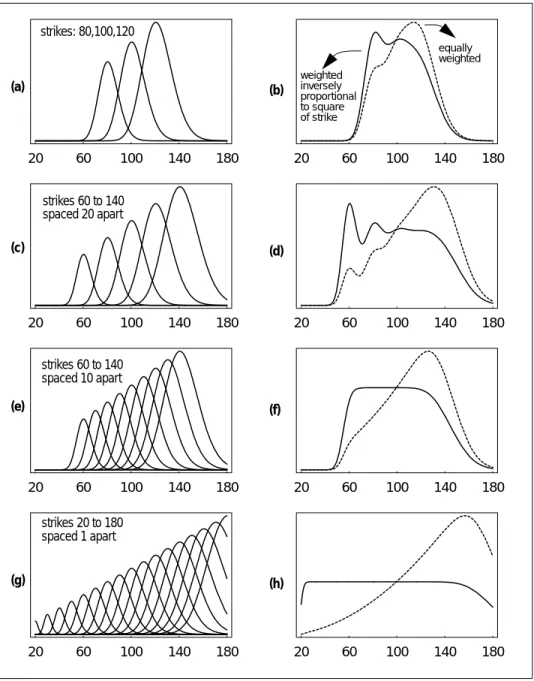
is the time to expiration (T−t), is the return volatility of the stock, is the stock’s variance, and is the total variance of the stock to expiration. (We have written the option value as a function of in order to make clear that all its dependence on both volatility and time to expiration is expressed in the combined variable .) We will call the exposure of an option to a stock’s variance V; it mea-sures the change in value of the position resulting from a change in variance2. Figure 1a shows a graph of howV varies with stock price S, for each of three different options with strikes 80, 100 and 120. For each strike, the variance exposure V is largest when the option is at the money, and falls off rapidly as the stock price moves in or out of the money.V is closely related to the time sensitivity or time decay of the option, because, in the Black-Scholes formula with zero interest rate, options values depend on the total variance .
If you want a long position in future realized variance, a single option is an imperfect vehicle: as soon as the stock price moves, your sensitiv-ity to further changes in variance is altered. What you want is a
portfo-2. Here, we define the sensitivity , where
. We will sometimes refer to V as “variance vega”. Note that d1depends only on the two combinations S/K and . V decreases extremely rapidly as S leaves the vicinity of the strike K.
CBS(S K, ,σ τ)
σ σ2
v = σ2τ
σ τ
σ τ
V
σ2 ∂
∂CBS S τ 2σ
--- d1 2
2
⁄ –
( )
exp 2π
---= =
d1 log(S K⁄ ) σ
2τ
( )⁄2 +
σ τ
---=
σ τ
lio whose sensitivity to realized variance is independent of the stock price S.
To obtain a portfolio that responds to volatility or variance indepen-dent of moves in the stock price, you need to combine options of many strikes. What combination of strikes will give you such undiluted vari-ance exposure?
Figure 1b shows the variance exposure for the portfolio consisting of all three option strikes in Figure 1a. The dotted line represents the sum of equally weighted strikes; the solid line represents the sum with weights in inverse proportion to the square of their strike. Figures 1c, e and g show the individual sensitivities to variance of increasing num-bers of options, each panel having the options more closely spaced. Fig-ures 1d, f and h show the sensitivity for the equally-weighted and strike-weighted portfolios. Clearly, the portfolio with weights inversely proportional to produces a V that is virtually independent of stock price S, as long as S lies inside the range of available strikes and far from the edge of the range, and provided the strikes are distributed evenly and closely.
Appendix A provides a mathematical derivation of the requirement that options be weighted inversely proportional to in order to achieve constant V. You can also understand this intuitively. As the stock price moves up to higher values, each additional option of higher strike in the portfolio will provide an additional contribution toV pro-portional to that strike. This follows from the formula in footnote 2, and you can observe it in the increasing height of the V-peaks in Fig-ure 1a. An option with higher strike will therefore produce aV contri-bution that increases with S. In addition, the contricontri-butions of all options overlap at any definite S. Therefore, to offset this accumulation of S-dependence, one needs diminishing amounts of higher-strike options, with weights inversely proportional to .
If you own a portfolio of options of all strikes, weighted in inverse pro-portion to the square of the strike level, you will obtain an exposure to variance that is independent of stock price, just what is needed to trade variance. What does this portfolio of options look like, and how does trading it capture variance?
Consider the portfolio of options of all strikes K and a single expiration τ, weighted inversely proportional to . Because
out-of-K2
K2
K2
Π(S,σ τ)
20 60 100 140 180 20 60 100 140 180
20 60 100 140 180 20 60 100 140 180
20 60 100 140 180 20 60 100 140 180
20 60 100 140 180 20 60 100 140 180
strikes: 80,100,120
equally weighted
strikes 60 to 140
strikes 20 to 180 spaced 1 apart
FIGURE 1. The variance exposure,V, of portfolios of call options of different
strikes as a function of stock price S. Each figure on the left shows the individual Vi contributions for each option of strike Ki. The corresponding figure on the right shows the sum of the contributions, weighted two different ways; the dotted line corresponds to an equally-weighted sum of options; the solid line corresponds to weights inversely proportional to K2, and becomes totally independent of stock price S inside the strike range
spaced 20 apart
strikes 60 to 140 spaced 10 apart
(a)
(c)
(e)
(g)
(b)
(d)
(f)
(h)
weighted inversely proportional to square of strike
the-money options are generally more liquid, we employ put options for strikes K varying continuously from zero up to some reference price S*, and call options for strikes varying continuously from S*to infinity3. You can think of S* as the approxi-mate at-the-money forward stock level that marks the boundary between liquid puts and liquid calls.
At expiration, when t=T,one can show that the sum of all the payoff values of the options in the portfolio is simply
(EQ 3)
where log( ) denotes the natural logarithm function, and STis the ter-minal stock price.
Similarly, at time t you can sum all the Black-Scholes options values to show that the total portfolio value is
(EQ 4)
where S is the stock price at time t. Note how little the value of the portfolio before expiration differs from its value at expiration at the same stock price. The only difference is the additional value due to half the total variance .
Clearly, the variance exposure ofΠis
(EQ 5)
To obtain an initial exposure of $1 per volatility point squared, you need to hold (2/T) units of the portfolioΠ.From now on, we will useΠto refer to the value of this new portfolio, namely
3. Formally, the expression for the portfolio is given by P S K( , ,σ τ)
C S K( , ,σ τ)
Π(S,σ τ) 1 K2
---C S K( , ,σ τ)
K>S*
∑
1K2
--- P S K( , ,σ τ)
K<S*
∑
+ =
Π(ST,0) ST–S* S*
--- ST S* --- log
– =
Π(S,σ τ) S–S* S*
--- S S* --- log
– σ
2τ 2
---+ =
σ2τ
V τ
2
(EQ 6)
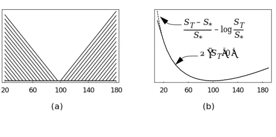
The first term in the payoff in Equation 6, (S −S*)/S*, describes 1/S* forward contracts on the stock with delivery price S*. It is not really an option; its value represents a long position in the stock (value S) and a short position in a bond (value S*), which can be statically replicated, once and for all, without any knowledge of the stock’s volatility. The second term, , describes a short position in a log contract4 with reference value S*, a so-called exotic option whose payoff is pro-portional to the log of the stock at expiration, and whose correct hedg-ing depends on the volatility of the stock. All of the volatility sensitivity of the weighted portfolio of options we have created is contained in the log contract.
Figure 2 graphically illustrates the equivalence between (1) the summed, weighted payoffs of puts and calls and (2) a long position in a forward contract and a short position in a log contract.
4. The log contract was first discussed in Neuberger (1994). See also Neu-berger (1996).
Π(S,σ τ) 2 T
---- S–S* S*
--- S S* --- log
– τ
T ----σ2
+ =
S S⁄ *
( )
log
–
20 60 100 140 180 20 60 100 140 180
FIGURE 2. An example that illustrates the equivalence at expiration
between (1) Π(ST,0) the weighted sum of puts and calls, with weight inversely proportional to the square of the strike, and (2) the payoff of a long position in a forward contract and a short position in a log contract. (a) Individual contributions to the payoff from put options with all integer strikes from 20 to 99, and call options with all integer strikes from 100 to 180. (b) The payoff of 1/100 of a long position in a forward contract with delivery price 100 and one short position in a log contract with reference value 100.
ST–S* S*
--- ST S* ---log
–
Π(ST,0)
Trading Realized Volatility with a Log Contract
For now, assume that we are in a Black-Scholes world where the implied volatility is the estimate of future realized volatility. If you take a position in the portfolioΠ, the fair value you should pay at time
when the stock price is S0is
At expiration, if the realized volatility turns out to have been , the initial fair value of the position captured by delta-hedging would have been
The net payoff on the position, hedged to expiration, will be
(EQ 7)
Looking back at Equation 2, you will see that by rehedging the position in log contracts, you have, in effect, been the owner of a position in a variance swap with fair strike Kvar = and face value $1. You will have profited (or lost) if realized volatility has exceeded (or been exceeded by) implied volatility.
The Vega, Gamma and Theta of a Log Contract
In Equation 6 we showed that, in a Black-Scholes world with zero interest rates and zero dividend yield, the portfolio of options whose variance vega is independent of the stock price S can be written
The term represents a long position in the stock and a short position in a bond, both of which can be statically hedged with no dependence on volatility. In contrast, the log( ) term needs continual dynamic rehedging. Therefore, let us concentrate on the log contract term alone, whose value at time t for a logarithmic payoff at time T is
(EQ 8)
σI
t = 0
Π0 2
T
---- S0–S* S*
--- S0 S* --- log
– +σ2I =
σR
Π0 2
T
---- S0–S* S*
--- S0 S* --- log
– +σR2 =
payoff = (σ2R–σ2I)
σ2I
Π(S, , ,σ t T) 2 T
---- S–S* S*
--- S S* --- log
– (T –t)
T ---σ2
+ =
S–S*
( )
L S( , , ,σ t T) 2 T ---- S
S* --- log
– (T–t)
T ---σ2
+ =
The sensitivities of the value of this portfolio are precisely appropriate for trading variance, as we now show.
The variance vega of the portfolio in Equation 8 is
(EQ 9)
The exposure to variance is equal to 1 at t = 0, and decreases linearly to zero as the contract approaches expiration.
The time decay of the log contract, the rate at which its value changes if the stock price remains unchanged as time passes, is
(EQ 10)
The contract loses time value at a constant rate proportional to its vari-ance, so that at expiration, all the initial variance has been lost.
The log contract’s exposure to stock price is
shares of stock. That is, since each share of stock is worth S, you need a constant long position in $(2/T) worth of stock to be hedged at any time. The gamma of the portfolio, the rate at which the exposure changes as the stock price moves, is
(EQ 11)
Gamma is a measure of the risk of hedging an option. The log con-tract’s gamma, being the sum of the gammas of a portfolio of puts and calls, is a smoother function of S than the sharply peaked gamma of a single option.
Equations 10 and 11 can be combined to show that
(EQ 12)
Equation 12 is the essence of the Black-Scholes options pricing theory. It states that the disadvantage of negative theta (the decrease in value with time to expiration) is offset by the benefit of positive gamma (the curvature of the payoff).
V T–t
T
---
=
θ 1
T ----σ2
– =
∆ 2
T ----1
S
----– =
Γ 2
T ---- 1
S2
---=
θ 1 2
---ΓS2σ2
Imperfect Hedges It takes an infinite number of strikes, appropriately weighted, to repli-cate a variance swap. In practice, this isn’t possible, even when the stock and options market satisfy all the Black-Scholes assumptions: there are only a finite number of options available at any maturity. Fig-ure 1 illustrates that a finite number of strikes fails to produce a uni-form V as the stock price moves outside the range of the available strikes. As long as the stock price remains within the strike range, trading the imperfectly replicated log contract will allow variance to accrue at the correct rate. Whenever the stock price moves outside, the reduced vega of the imperfectly replicated log contract will make it less responsive than a true variance swap.
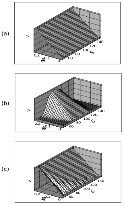
Figure 3 shows how the variance vega of a three-month variance swap is affected by imperfect replication. Figure 3a shows the ideal variance vega that results from a portfolio of puts and calls of all strikes from zero to infinity, weighted in inverse proportion to the strike squared. Here the variance vega is independent of stock price level, and decreases linearly with time to expiration, as expected for a swap whose value is proportional to the remaining variance at any time. Figure 3b shows strikes from $75 to $125, uniformly spaced $1 apart. Here, deviation from constant variance vega develops at the tail of the strike range, and the deviation is greater at earlier times. Finally, Fig-ure 3c shows the vega for strikes from $20 to $200, spaced $10 apart. Now, although the range of strikes is greater, the coarser spacing causes the vega surface to develop corrugations between strike values that grow more pronounced closer to expiration.
The Limitations of the Intuitive Approach
A variance swap has a payoff proportional to realized variance. In this section, assuming the Black-Scholes world for stock and options mar-kets, we have shown that the dynamic, continuous hedging of a log con-tract produces a payoff whose value is proportional to future realized variance. We have also shown that you can use a portfolio of appropri-ately weighted puts and calls to approximate a log contract.
The somewhat intuitive derivations in this section have assumed that interest rates and dividend yields are zero, but it is not hard to gener-alize them. We have also assumed that all the Black-Scholes assump-tions hold. In practice, in the presence of an implied volatility skew, it is difficult to extend these argument clearly. Therefore, we move on to a more general and rigorous derivation of the value of variance swaps based on replication. Many of the results will be similar, but the condi-tions under which they hold, and the correct answers when they do not hold, will be more easily understandable.
FIGURE 3. The variance vega,V ,of a portfolio of puts and calls, weighted inversely proportional to the square of the strike level, and chosen to replicate a three-month variance swap. (a) An infinite number of strikes. (b) Strikes from $75 to $125, uniformly spaced $1 apart. (c) Strikes from $20 to $200, uniformly spaced $10 apart.
v
60 80
100 120
140
S
0 0.1 0.2
τ
v
60 80
100 120
140
S
0 0.1 0.2
τ
v
60 80
100 120
140
S
0 0.1 0.2
τ
V
V
V
(a)
(b)
REPLICATING VARIANCE SWAPS: GENERAL RESULTS
In the previous section, we explained how to replicate a variance swap by means of a portfolio of options whose payoffs approximate a log con-tract. Although our explanation depended on the validity of the Black-Scholes model, the result – that the dynamic hedging of a log contract captures realized volatility – holds true more generally. The only assumption we will make about the future underlyer evolution is that it is diffusive, or continuous – this means that no jumps are allowed. (In a later section, we will consider the effects of discontinuous stock price movements on the success of the replication.) Therefore, we assume that the stock price evolution is given by
(EQ 13)
Here, we assume that the driftµand the continuously-sampled volatil-ity σ are arbitrary functions of time and other parameters. These assumptions include, but are not restricted to, implied tree models in which the volatility is a function of stock price and time only. For simplicity of presentation, we assume the stock pays no dividends; allowing for dividends does not significantly alter the derivation. The theoretical definition of realized variance for a given price history is the continuous integral
(EQ 14)
This is a good approximation to the variance of daily returns used in the contract terms of most variance swaps.
Conceptually, valuing a variance forward contract or “swap” is no dif-ferent than valuing any other derivative security. The value of a for-ward contract F on future realized variance with strike K is the expected present value of the future payoff in the risk-neutral world:
(EQ 15)
Here r is the risk-free discount rate corresponding to the expiration date T, and E[ ] denotes the expectation.
The fair delivery value of future realized variance is the strike for which the contract has zero present value:
(EQ 16)
dSt St
--- = µ(t ..., )dt+σ(t ..., )dZt
σ(S t, )
V 1
T
---- σ2(t,…)dt 0
T
∫
=
F = E e[ –rT(V–K)]
Kvar
If the future volatility in Equation 13 is specified, then one approach for calculating the fair price of variance is to directly calculate the risk-neutral expectation
(EQ 17)
No one knows with certainty the value of future volatility. In implied tree models5, the so-called local volatility consistent with all current options prices is extracted from the market prices of traded stock options. You can then use simulation to calculate the fair vari-ance Kvaras the average of the experienced variance along each simu-lated path consistent with the risk-neutral stock price evolution given of Equation 13, where the driftµis set equal to the riskless rate. The above approach is good for valuing the contract, but it does not provide insight into how to replicate it. The essence of the replication strategy is to devise a position that, over the next instant of time, gen-erates a payoff proportional to the incremental variance of the stock during that time6.
By applying Ito’s lemma to , we find
(EQ 18)
Subtracting Equation 18 from Equation 13, we obtain
(EQ 19)
in which all dependence on the drift has cancelled. Summing Equa-tion 19 over all times from 0 to T, we obtain the continuously-sampled variance
5. See, for example, Derman and Kani (1994), Dupire (1994) and Derman, Kani and Zou (1996).
6. This approach was first outlined in Derman, Kamal, Kani, and Zou (1996). For an alternative discussion, see Carr and Madan (1998).
Kvar 1
T
---- E σ2(t,…)dt 0
T
∫
=
σ(S t, )
St log
d(logSt) µ 1 2 ---σ2
–
dt σdZ t
+ =
dSt St
---–d(logSt) 1 2 ---σ2dt
=
(EQ 20)
This mathematical identity dictates the replication strategy for vari-ance. The first term in the brackets can be thought of as the net out-come of continuous rebalancing a stock position so that it is always instantaneously long shares of stock worth $1. The second term represents a static short position in a contract which, at expiration, pays the logarithm of the total return. Following this continuous rebal-ancing strategy captures the realized variance of the stock from incep-tion to expiraincep-tion at time T. Note that no expectaincep-tions or averages have been taken – Equation 20 guarantees that variance can be captured no matter which path the stock price takes, as long as it moves continu-ously.
Valuing and Pricing the Variance Swap
Equation 20 provides another method for calculating the fair variance. Instead of averaging over future variances, as in Equation 17, one can take the expected risk-neutral value of the right-hand side of Equation 20 to obtain the cost of replication directly, so that
(EQ 21)
The expected value of the first term in Equation 21 accounts for the cost of rebalancing. In a risk-neutral world with a constant risk-free rate r, the underlyer evolves according to:
(EQ 22)
so that the risk-neutral price of the rebalancing component of the hedg-ing strategy is given by
(EQ 23)
This equation represents the fact that a shares position, continuously rebalanced to be worth $1, has a forward price that grows at the risk-less rate.
V 1
T ---- σ2dt
0 T
∫
≡2 T
---- dSt St ---0 T
∫
STS0 ---log
– =
1/St
Kvar 2
T
---- E dSt St ---0 T
∫
STS0 ---log
– =
St d
St
--- = rdt+σ(t,…)dZ
E dSt
St ---0 T
As there are no actively traded log contracts for the second term in Equation 21, one must duplicate the log payoff, at all stock price levels at expiration, by decomposing its shape into linear and curved nents, and then duplicating each of these separately. The linear compo-nent can be duplicated with a forward contract on the stock with delivery time T; the remaining curved component, representing the quadratic and higher order contributions, can be duplicated using stan-dard options with all possible strike levels and the same expiration time T.
For practical reasons we want to duplicate the log payoff with liquid options – that is, with a combination of out-of-the-money calls for high stock values and out-of-the-money puts for low stock values. We intro-duce a new arbitrary parameter S* to define the boundary between calls and puts. The log payoff can then be rewritten as
(EQ 24)
The second term is constant, independent of the final stock price ST, so only the first term has to be replicated.
The following mathematical identity, which holds for all future values of ST, suggests the decomposition of the log-payoff:
(EQ 25)
Equation 25 represents the decomposition of a log payoff into a portfo-lio consisting of:
• a short position in forward contracts struck at S*;
• a long position in put options struck at K, for all strikes from 0 to S*; and
• a similar long position in call options struck at K, for all strikes from S* to .
All contracts expire at time T. Figure 4 shows this decomposition sche-matically.
ST S0
---log ST
S*
---log S*
S0 ---log
+ =
S*⁄S0
( )
log
ST S* ---log
– ST–S*
S*
--- (forward contract)
– =
1 K2
--- Max K( –ST,0)dK 0
S*
∫
+ (put options)
1 K2
--- Max S( T–K,0)dK (call options) S*
∞
∫
+
1 S⁄ *
( )
1 K⁄ 2
( )
1 K⁄ 2
( )
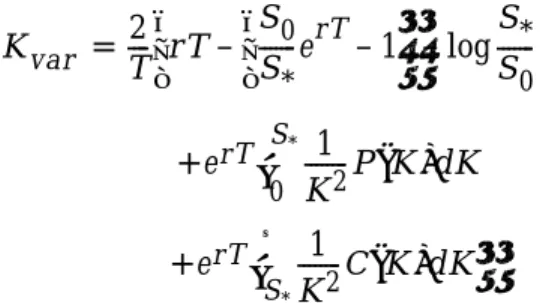
The fair value of future variance can be related to the initial fair value of each term on the right hand side of Equation 21. By using the identi-ties in Equations 23 and 25, we obtain
(EQ 26)
where P(K) and (C(K)), respectively, denote the current fair value of a put and call option of strike K. If you use the market prices of these options, you obtain an estimate of the current market price of future variance.
This approach to the fair value of future variance is the most rigorous from a theoretical point of view, and makes less assumptions than our intuitive treatment in the section on page 6. Equation 26 makes pre-cise the intuitive notion that implied volatilities can be regarded as the market’s expectation of future realized volatilities. It provides a direct connection between the market cost of options and the strategy for cap-turing future realized volatility, even when there is an implied volatility skew and the simple Black-Scholes formula is invalid.
Kvar 2
T
---- rT S0 S*
---erT–1
S*
S0 ---log
– –
=
erT 1
K2
--- P K( )dK 0
S*
∫
+
erT 1
K2
---C K( )dK S*
∞
∫
+
FIGURE 4. Replication of the log payoff. (a) The payoff of a short position in a
log contract at expiration. (b) Dashed line: the linear payoff at expiration of a forward contract with delivery price S*; Solid line: the curved payoff of
calls struck above S* and puts struck below S*. Each option is weighted by
the inverse square of its strike. The sum of the payoffs for the dashed and solid lines provide the same payoff as the log contract.
S*
S* ST
S* ---log
–
ST–S* S*
---–
portfolio of options
AN EXAMPLE OF A VARIANCE SWAP
We now present a detailed practical example. Suppose you want to price a swap on the realized variance of the daily returns of some hypo-thetical equity index. The fair delivery variance is determined by the cost of the replicating strategy discussed in the previous section. If you could buy options of all strikes between zero and infinity, the fair vari-ance would be given by Equation 26 with some choice of S*, say S*= S0. In practice, however, only a small set of discrete option strikes is avail-able, and using Equation 26 with only a few strikes leads to apprecia-ble errors. Here we suggest a better approximation.
We start with the definition of fair variance given by Equation 21, which can be written as
Taking expectations, this becomes
(EQ 27)
where is the present value of the portfolio of options with payoff at expiration given by
(EQ 28)
Suppose that you can trade call options with strikes Kic such that and put options with strikes Kip such that
In Appendix A we derive the formula that determines how many options of each strike you need in order to approximate the payoff f(ST) by piece-wise linear options payoffs. The procedure in Appendix A guarantees that these payoffs will always exceed or match the value of the log contract, but never be worth less. Once these weights are calcu-lated, is obtained from
(EQ 29)
We now illustrate this procedure with a concrete numerical example.
Kvar 2
T
---- E dSt St ---0 T
∫
ST–S* S*---– S*
S0
--- ST–S* S*
--- ST S* ---log
– +
log
–
≡
Kvar 2
T
---- rT S0 S*
---erT–1
S*
S0 ---log
–
– +erTΠCP
=
ΠCP
f S( T) 2 T
---- ST–S* S*
--- ST S* ---log
–
=
K0 = S*<K1c<K2c<K3c<... K0 = S*>K1 p>K2 p>K3 p>...
ΠCP
ΠCP w K( ip)P S K( , ip) w K( ic)C S K( , ic) i
∑
+
i
∑
TABLE 1. The portfolio of European-style put and call options used for calculating the cost of capturing realized variance in the presence of the implied volatility skew with a discrete set of options strikes.
Assume that the index level S0is 100, the continuously compounded annual riskless interest rate r is 5%, the dividend yield is zero, and the maturity of the variance swap is three months (T = 0.25. Suppose that
Strike Volatility Weight
Value per Option
Contribution
PUTS
50 30 163.04 0.000002 0.0004
55 29 134.63 0.00003 0.0035
60 28 113.05 0.0002 0.0241
65 27 96.27 0.0013 0.1289
70 26 82.98 0.0067 0.5560
75 25 72.26 0.0276 1.9939
80 24 63.49 0.0958 6.0829
85 23 56.23 0.2854 16.0459
90 22 50.15 0.7384 37.0260
95 21 45.00 1.6747 75.3616
100 20 20.98 3.3537 70.3615
C
ALLS
100 20 19.63 4.5790 89.8691
105 19 36.83 2.2581 83.1580
110 18 33.55 0.8874 29.7752
115 17 30.69 0.2578 7.9130
120 16 28.19 0.0501 1.4119
125 15 25.98 0.0057 0.1476
130 14 24.02 0.0003 0.0075
135 13 22.27 0.000006 0.0001
you can buy options with strikes in the range from 50 to 150, uniformly spaced 5 points apart. We assume that at-the-money implied volatility is 20%, with a skew such that the implied volatility increases by 1 vola-tility point for every 5 point decrease in the strike level. In Table 1 we provide the list of strikes and their corresponding implied volatilities. We then show the weights, the value of each individual option and the contribution of each strike level to the total cost of the portfolio. At the bottom of the table we show the total cost of the options portfolio, . It is clear from Table 1 that most of the cost comes from options with strikes near the spot value. Although the number of options which are far out of the money is large, their value is small and contributes little to the total cost.
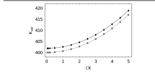
The cost of capturing variance is now simply calculated using Equation 27 with the result . This is not strictly the fair vari-ance; because the procedure of approximating the log contract in Appendix A always over-estimates the value of the log contract, this value is higher than the true theoretical value for the fair variance obtained by approximating the log contract with a continuum of strikes. In Figure 5 we illustrate the cost of variance as function of the spacing between strikes, for two cases, with and without a volatility skew. You can see that as the spacing between strikes approaches zero, the cost of capturing variance approaches the theoretically fair vari-ance.
0 1 2 3 4 5
DK 400
405 410 415 420
Kvar
FIGURE 5. Convergence of Kvar, the cost of capturing variance with a
discrete set of strikes, towards the fair value of variance as a function of
∆K, the spacing between strikes. The line with square symbols shows the convergence for no skew, with all implied volatilities at the same value of 20%. The theoretical fair variance for∆K = 0 is then (20)2= 400. The line with diamond symbols shows similar convergence to a higher fair variance of about 402, the extra contribution coming from the effect of the skew.
ΠCP = 419.8671
EFFECTS OF THE VOLATILITY SKEW
The general strategy discussed in the previous section can be used to determine the fair variance and the hedging portfolio from the set of available options and their implied volatilities. Here we discuss the effects of a volatility skew on the fair variance. We assume that there is no term structure and consider two different skew parameterizations, both of which resemble typical index skews. The first is a skew that varies linearly with the strike of the option, the second a skew that varies linearly with the Black-Scholes delta. In both cases we will com-pare the numerically correct value of fair variance, computed from Equation 26, with an approximate analytic formula that we derive. This formula provides a good rule of thumb for a quick estimate of the impact of the volatility skew on the fair variance.
Skew Linear in Strike We first consider a skew for which the implied volatility varies linearly with strike, so that
(EQ 30)
HereΣ0is the implied volatility of an option struck at the forward. The steepness of the skew is determined by the slope b, with a positive value indicating a higher volatility for strikes below the forward. Note that this parametrization cannot hold for all strikes, because, for a large enough value of K, the implied volatility would become negative7. A value of b = 0.2 means that the implied volatility corresponding to a strike 10% below the forward, for example, is 2 volatility points higher than Σ0. In Appendix B we derive the following approximate formula for the fair variance of the contract with time to expiration T:
(EQ 31)
The skew increases the value of the fair variance above the at-the-money-forward level of volatility, and the size of the increase is propor-tional to time to maturity and the square of the skew slope. (Note that b in Equation 30 has the same dimension as volatility, so that b2T is a dimensionless parameter, and therefore a natural candidate for the order of magnitude of the percentage correction to Kvar. Note also that there is no term in Equation 31. This approximation works best for short maturities and skews that are not too steep.
7. Note that for large values of K, where this parameterization is invalid, the options prices in Equation 26 are negligible and therefore do not affect the value of the fair variance.
Σ( )K Σ0 bK–SF SF
---– =
Kvar≈Σ02(1+3T b2+....)
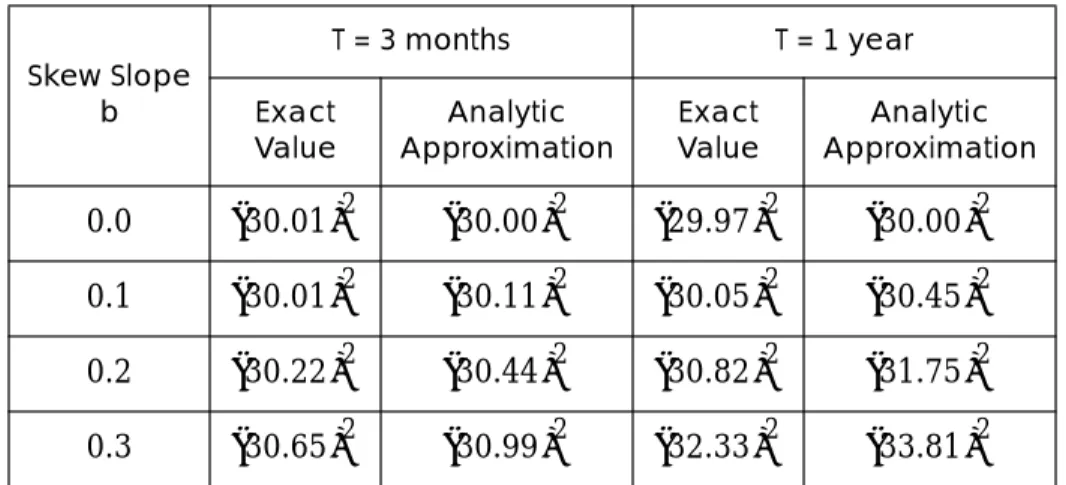
In Table 2 we compare the exact results for fair variance, computed numerically, with the approximate values given by the analytic for-mula in Equation 31.
TABLE 2.Comparison of the exact fair variance, computed numerically, with
the approximate analytic formula of Equation 31. We assumeΣ0= 30%, S = 100, the continuously compounded annual discount rate r = 5%, zero dividend yield, and use strikes evenly spaced one point apart from K = 10 to K = 200 to replicate the log payoff.
Figure 6 contains a graph of these results. We see excellent agreement in the case of the three-month variance swap, and reasonable agree-ment for one year.
Skew Slope b
T = 3 months T = 1 year Exact
Value
Analytic Approximation
Exact Value
Analytic Approximation
0.0 0.1 0.2 0.3
30.01
( )2 (30.00)2 (29.97)2 (30.00)2 30.01
( )2
30.11 ( )2
30.05 ( )2
30.45 ( )2 30.22
( )2 (30.44)2 (30.82)2 (31.75)2 30.65
( )2
30.99 ( )2
32.33 ( )2
33.81 ( )2
0.1 0.2 0.3 b
900 950 1000 1050 1100 1150
Kv
a
r
0.1 0.2 0.3 b
900 950 1000 1050 1100 1150
Kv
a
r
FIGURE 6. Comparison of the exact value of fair variance, Kvar, with the
approximate value from the formula of Equation 31, as a function of the skew slope b. The thin line with squares shows the exact values obtained by replicating the log-payoff. The thick line depicts the approximate value given by Equation 31. (a) three-month variance swap. (b) one-year variance swap.
Skew Linear in Delta Next we consider a skew that varies linearly with the Black-Scholes delta of the option, so that:
(EQ 32)
Here ∆p is the Black-Scholes exposure of a put option, given by , where d1 is defined in Footnote 2, is the implied volatility of a “50-delta” put option and b is the slope of the skew – that is, the change in the skew per unit delta. This parameter b is not the same as the b in the previous section. In particular, there is an implicit dependence on the time to expiration in the formula of Equation 32, because of the∆pterm, which was absent from Equation 30. Since∆pis bounded, the implied volatility is always positive provided b < 2Σ0. This restriction is irrelevant, since Equation 32 leads to arbitrage vio-lation before b reaches this limit. In practice, this parameterization leads to more realistic skews than those produced by the linear-strike formula.
Appendix C presents a detailed derivation of the following approximate formula for the fair variance of the contract with time to expiration T:
(EQ 33)
Here, in contrast to the skew linear in strike, the first-order correction is of magnitude , because a variation linear in delta about the at-the-money-forward strike is not equivalent to a variation linear in strike.
Σ ∆( p) Σ0 b ∆p 1 2
---+
+ =
∆p = –N(–d1) Σ0
Kvar Σ02 1 1 π
---b T 1 12 ---b
2
Σ02 --- ....
+ + +
≈
b T
-1 -0.75 -0.5 -0.25 0 ∆p
20 25 30 35 40
Σ
60 80 100 120 140
K
20 25 30 35 40
Σ
FIGURE 7. (a) A volatility skew that varies linearly in delta. (b) The
corresponding skew plotted as a function of strike. We have assumed that the stock price S is 100, the continuously compounded annual discount rate r is 5%, the term to maturity is three months, and the skew slope is 0.2.
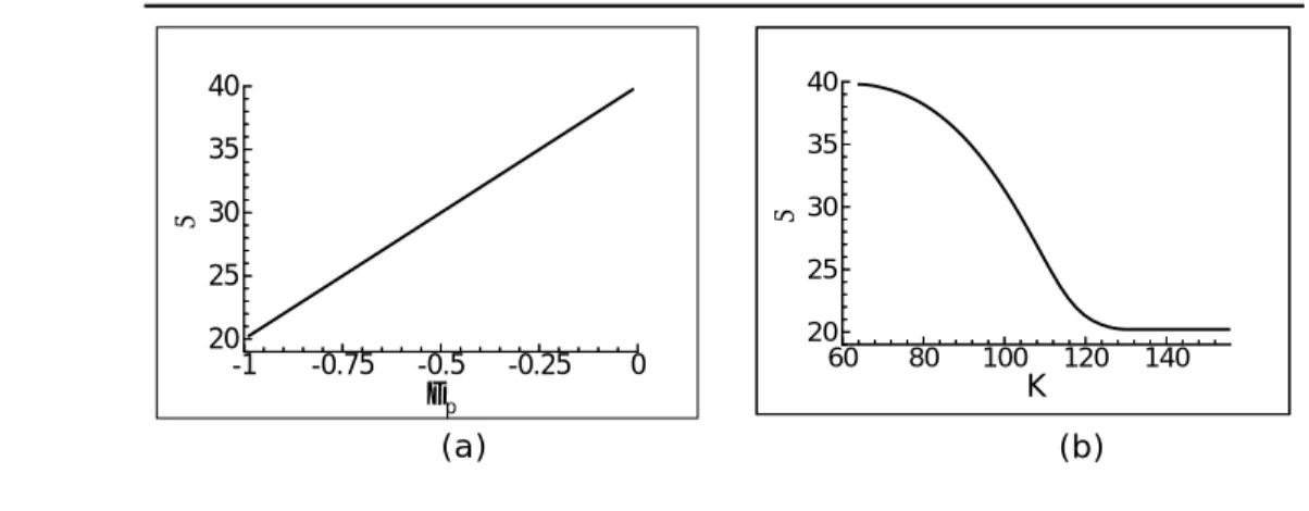
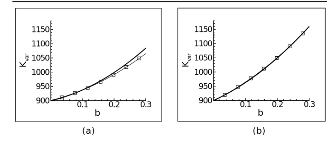
First, we convert the skew by delta in Equation 32 into a skew by strike, as displayed in Figure 7. Again, we compare the exact results computed according to Appendix A with the approximate values given by Equation 33. In Table 3 we compare the results for fair variance, computed numerically, with the approximate values given by the ana-lytic formula in Equation 33. The anaana-lytic formula works very well for the three-month variance swap, and truly impressively for the one-year swap, as displayed in Figure 8.
TABLE 3.Comparison of the fair variance, computed numerically, with the
approximate analytic formula of Equation 33. We assumeΣ0= 30%, S = 100, the continuously compounded annual discount rate r = 5%, zero dividend yield, and use strikes evenly spaced one point apart from K = 10 to K = 200 to replicate the log payoff.
Skew Slope b
T = 3 months T = 1 year Exact
Value
Analytic Approximation
Exact Value
Analytic Approximation
0.0 0.1 0.2 0.3
30.01 ( )2
30.00 ( )2
29.97 ( )2
30.00 ( )2 30.61
( )2 (30.62)2 (31.06)2 (31.03)2 31.49
( )2
31.60 ( )2
32.42 ( )2
32.40 ( )2 32.64
( )2 (32.93)2 (34.06)2 (34.06)2
0.1 0.2 0.3 b
900 950 1000 1050 1100 1150
Kv
a
r
0.1 0.2 0.3 b
900 950 1000 1050 1100 1150
Kv
a
r
FIGURE 8. Comparison of the exact value of fair variance, Kvar, with the
approximate value from the formula of Equation 33, as a function of the skew slope b. The thin line with squares shows the exact values obtained by replicating the log-payoff. The thick line depicts the approximate value given by Equation 33. (a) Three-month variance swap. (b) One-year variance swap.
PRACTICAL PROBLEMS WITH REPLICATION
We have shown in Equation 20 that a variance swap is theoretically equivalent to a dynamically adjusted, constant-dollar exposure to the stock, together with a static long position in a portfolio of options and a forward that together replicate the payoff of a log contract. This portfo-lio strategy captures variance exactly, provided the portfoportfo-lio of options contains all strikes between zero and infinity in the appropriate weight to match the log payoff, and provided the stock price evolves continu-ously.
Two obvious things can go wrong. First, you may be able to trade only a limited range of options strikes, insufficient to accurately replicate the log payoff. Second, the stock price may jump. Both of these effects cause the strategy to capture a quantity that is not the true realized variance. We will focus on the effects of these two limitations below, though other practical issues, like liquidity, may also corrupt the ideal strategy.
Imperfect Replication Due to Limited Strike Range
Variance replication requires a log contract. Since log contracts are not traded in practice, we replicate the payoff with traded standard options in a limited strike range. Because these strikes fail to duplicate the log contract exactly, they will capture less than the true realized variance. Therefore, they have lower value than that of a true log contract, and so produce an inaccurate, lower estimate of the fair variance.
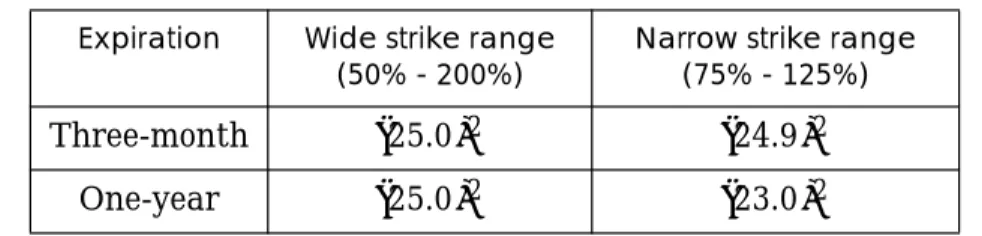
In Table 4 below we show how the estimated value of fair variance is affected by the range of strikes that make up the replicating portfolio. The fair variances are estimated from (1) a replicating portfolio with a narrow range of strikes, ranging from 75% to 125% of the initial spot level, and (2) a portfolio with a wide range of strikes, from 50% to 200% of the initial spot level. In both cases the strikes are uniformly spaced, one point apart. (The fair variance is calculated according to Equation 26, except that the integrals are replaced by sums over the available option strikes whose weights are chosen according to the procedure of Appendix A). We assume here that implied volatility is 25% per year for all strikes, with no volatility skew, so that all options are valued at the same implied volatility. We also assume a continuously com-pounded annual interest rate of 5%.
For both expirations, the wide strike range accurately approximates the actual square of the implied volatility. However, the narrow strike range underestimates the fair variance, more dramatically so for longer expirations.
TABLE 4. The effect of strike range on estimated fair variance.
In the section entitledReplicating Variance Swaps: First Stepson page 6, we have already discussed one approach to understanding why the narrow strike range fails to capture variance. As shown in Figure 3, the vega and gamma of a limited strike range both fall to zero when the index moves outside the strike range, and the strategy then fails to accrue realized variance as the stock price moves. Consequently, the esti-mated variance is lower than the true fair value for both expirations above, and the reduction in value is greater for the one-year case. Over a longer time period it is more likely that the stock price will evolve outside the strike range.
In essence, capturing variance requires owning the full log contract, whose duplication demands an infinite range of strikes. If you own a limited number of strikes, still appropriately weighted, you pay less than the full value, and, when the stock price evolves into regions where the curvature of the portfolio is insufficiently large, you capture less than the full realized variance, even if no jumps occur and the stock always moves continuously. In order to keep capturing variance, you need to maintain the curvature of the log contract at the current stock price, whatever value it takes.
A simpler way of understanding why a narrow strike range leads to a lower fair variance is to compare the payoff of the narrow-strike repli-cating portfolio at expiration to the terminal payoff that the portfolio is attempting to replicate, that is, the nonlinear part of the log payoff:
(EQ 34)
Figure 9 displays the mismatch between the two payoffs. The narrow-strike option portfolio matches the curved part of the log payoff well at stock price levels between the range of strikes, that is, from 75 to 125. Beyond this range, the option portfolio payoff remains linear, always growing less rapidly than the nonlinear part of the log contract. The lack of curvature (or gamma, or vega) in the options portfolio outside
Expiration Wide strike range (50% - 200%)
Narrow strike range (75% - 125%)
Three-month One-year
25.0
( )2 (24.9)2
25.0
( )2 (23.0)2
ST–S0 S0
--- ST S0 ---log
the narrow strike range is responsible for the inability to capture vari-ance.
The Effect of Jumps on a Perfectly Repli-cated Log Contract
When the stock price jumps, the log contract may no longer capture realized volatility, for two reasons. First, if the log contract has been approximately replicated by only a finite range of strikes, a large jump may take the stock price into a region in which variance does not accrue at the right rate. Second, even with perfect replication, a discon-tinuous stock-price jump causes the variance-capture strategy of Equa-tion 20 to capture an amount not equal to the true realized variance. In reality, both these effects contribute to the replication error. In this sec-tion, we focus only on the second effect and examine the effects of jumps assuming that the log-payoff can be replicated perfectly with options.
For the sake of discussion, from now on we will assume that we are short the variance swap, which we will hedge by following a discrete version of the variance-capture strategy
(EQ 35)
where is the change in stock price between successive
observations. Rather than continuously rebalance as the stock price moves, we instead adjust the exposure to (2/T) dollars worth of stock only when a new stock price is recorded for updating the realized vari-ance.
Because of the additive properties of the logarithm function, the termi-nal log payoff is equivalent to a daily accumulation of log payoffs:
50 100 150 200
ST
T
e
rm
in
a
l
p
a
y
o
ff
FIGURE 9. Comparison of the terminal payoff of the narrow-strike replicating
portfolio (dashed line) and the nonlinear part of the log-payoff (solid line).
V 2
T
---- ∆Si Si–1 ---i=1
N
∑
STS0 ---log
– =
(EQ 36)
Suppose that all but one of the daily price changes are well-behaved – that is, all changes are diffusive, except for a single jump event. We characterize the jump by the parameter , the percentage jump
down-wards, from ; a jump downwards of 10% corresponds to J
= 0.1. A jump up corresponds to a value J < 0.
The contribution of this one jump to the variance is easy to isolate, because variance is additive; the total (un-annualized) realized vari-ance for a zero-mean contract is the sum
(EQ 37)
The contribution of the jump to the realized total variance is given by:
(EQ 38)
On the other hand, the impact of the jump on the quantity captured by our variance replication strategy in Equation 36 is
(EQ 39)
In the limit that the jump size J is small enough to be regarded as part of a continuous stock evolution process, the right hand side of Equation 39 does reduce to the contribution of this (now small) move to the true realized variance. It is only because J is not small that the variance capture strategy is inaccurate. Therefore, the replication error, or the P&L (profit/loss) due to the jump for a short position in a variance swap hedged by a long position in a variance-capture strategy is
(EQ 40)
To understand this result better, it is helpful to expand the log function as a series in J:
(EQ 41)
V 2
T
---- ∆Si Si–1
--- Si Si–1 ---log
–
i=1 N
∑
=
J S→S 1( –J)
V 1
T
---- ∆Si Si–1
---
2
∑
1T
---- ∆Si
Si–1
---
2 1 T ---- ∆S
S --- 2
jump
+
no jumps
∑
= =
1 T ---- ∆S
S --- 2
jump J2 T ---= 2 T ---- ∆Si
Si–1
--- Si Si–1 ---log – jump 2 T
----[–J–log(1–J)]
=
P&L due to jump =2 T
----[–J–log(1–J)] J2 T
---–
1–J
( )
log
– J J2
2 --- J3
3 --- …
+ + + =