Learning Motion Categories using both Semantic and Structural Information
Shu-Fai Wong, Tae-Kyun Kim and Roberto Cipolla
Department of Engineering,
University of Cambridge,
Cambridge, CB2 1PZ, UK
{sfw26, tkk22, cipolla}@eng.cam.ac.uk
Abstract
Current approaches to motion category recognition typ-ically focus on either full spatiotemporal volume analysis (holistic approach) or analysis of the content of spatiotem-poral interest points (part-based approach). Holistic ap-proaches tend to be more sensitive to noise e.g. geomet-ric variations, while part-based approaches usually ignore structural dependencies between parts. This paper presents a novel generative model, which extends probabilistic latent semantic analysis (pLSA), to capture both semantic (con-tent of parts) and structural (connection between parts) in-formation for motion category recognition. The structural information learnt can also be used to infer the location of motion for the purpose of motion detection. We test our al-gorithm on challenging datasets involving human actions, facial expressions and hand gestures and show its perfor-mance is better than existing unsupervised methods in both tasks of motion localisation and recognition.
1. Introduction
With the abundance of multimedia data, there is a great demand for efficient organisation of images and videos in an unsupervised manner so that the data can be searched easily. In this paper, we will focus on the motion categorisation problem for video organisation.
Among traditional approaches to motion categorisation, computing correlation between two spatiotemporal (ST) volumes (i.e. whole video inputs) is the most straight-forward method. Various correlation methods such as cross correlation between optical flow descriptors [4] and a con-sistency measure between ST volumes from their local in-tensity variations [13] have been proposed. Although this approach is easy to understand and implement and makes a good use of geometrical consistency, it cannot handle large geometric variation between intra-class samples, mov-ing cameras and non-stationary backgrounds, and it is also
computational demanding for motion localisation in large ST volumes.
Instead of performing the above holistic analysis, many researchers have adopted an alternative, part-based ap-proach. This approach uses only several ‘interesting’ parts of the whole ST volume for analysis and thus avoids problems such as non-stationary backgrounds. The parts can be trajectories [16] or flow vectors [15, 5] of cor-ners, profiles generated from silhouettes [1] and ST inter-est points [9, 3, 8]. Among them, ST interinter-est points can be obtained more reliably and thus be widely adopted in motion categorisation where discriminative classifiers such as support vector machines (SVM) [12] and boosting [8], and generative models such as probabilistic latent seman-tic analysis (pLSA) [11] and specific graphical models [2] have been exploited. When considering a huge amount of unlabelled video, generative models, which require the least amount of human intervention, seem to be the best choice.
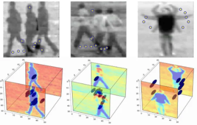
Currently used generative models for part-based motion analysis still have room for improvement. For instance, Boiman and Irani’s work [2] is designed specifically for irregularity detection only, and Niebles et al.’s work [11] ignores structural (or geometrical) information which may be useful for motion categorisation. As shown in Figure 1, 3D (ST) interest regions generated by walking sequences geometrically distribute in a different way than those from a hand waving sequence. Adding structural information into the generative models, however, is not a trivial task and may increase time complexity dramatically. Inspired by the 2D image categorisation works of Fergus et al. [6] and Leibe et al. [10], we first extend the generative models for 2D im-age analysis, which uses structural information, to 3D video analysis, and then propose a novel generative model called pLSA with an implicit shape model (pLSA-ISM) which can make use of both semantic (the content of ST interest re-gions orcuboids) and structural (geometrical relationship between cuboids) information for efficient inference of mo-tion category and locamo-tion. A retraining algorithm which can improve an initial model using unsegmented data in an
unsupervised manner is also proposed in this paper. Next section will describe the proposed model in details.
Figure 1. Top row shows superposition images of two walking se-quences and a hand waving sequence. Spatiotemporal (ST) inter-est points (detected by method proposed in [3]) are also displayed. Bottom row shows the 3D visualisation of those ST points.
2. Approach
Before describing our approach, we first review pLSA and its variations applied in 2D object categorisation.
(a) pLSA (b) ABS-pLSA
(c) TSI-pLSA (d) pLSA-ISM
Figure 2. Graphical models of various pLSA described.
2.1. Classical pLSA
Classical pLSA was originally used in document analy-sis. Following the notation used in Sivic et al. [14] and referring to Figure 2(a), we have a set of D Documents and each of them contains a set ofNd Words. All words
from the set of D documents can be vector quantitised into W word classes (words) which form a code-book. The corpus of documents can then be represented by a co-occurrence matrix of size W × D, with entry
n(w, d) indicating the number of code-word w in docu-mentd. Apart from documents and words which are
ob-servable from data, we also have an unobob-servable variable,
z, to describeZ Topics covered in documents and associ-ated with words. The pLSA algorithm can be used to learn the associations:P(w|z)(words that can be generated from a topic) andP(z|d)(the topic of a document) through an Expectation-Maximisation (EM) algorithm [7] applied on the co-occurrence matrix.
The pLSA model can be applied in 2D image analy-sis [14] by replacing ‘words’ by interestpatchesand ‘doc-uments’ byimages, and in 3D motion analysis [11] by re-placing ‘words’ bycuboidsand ‘documents’ byvideos.
2.2. Absolute position pLSA(ABS-pLSA)
In image analysis, structural information (i.e. geometric relationship between interest patches) can be used to im-prove the original pLSA model. Fergus et al. [6] proposed to quantitise location measurement of patches in an absolute coordinate frame to a discrete variablexabs and to learn a joint density P((w, xabs)|z)instead of P(w|z) in pLSA. Referring to Figure 2(b), the new model can be trained us-ing the standard pLSA by substitutus-ing (w, xabs) intowof the original pLSA model.
2.3. Translation and Scale Invariant pLSA
(TSI-pLSA)
ABS-pLSA is simple to implement, but sensitive to translation and scale changes. Thus, Fergus et al. [6] ex-tended it to be translation and scale invariant by introduc-ing a latent variablecabs (in an absolute coordinate frame) for representing centroid locations (See Figure 2(c)). In short, relative location xrel (w.r.t. centroid) is used
in-stead of an absolute one so that the model built is trans-lation and scale invariant. To avoid doing computational expensive inference on estimating centroid locations, Fer-gus et al. proposed to use a sampling scheme where cen-troid samples are obtained by clustering interest patches based on their likelihood P(w|z) on a certain topic and their spatial locations. The term P((w, xrel)|z)(with rel-ative locationx) can then be obtained by marginalisation,
cP((w, xrel)|cabs, z)P(cabs)using the centroid samples.
2.4. pLSA with implicit shape model (pLSA-ISM)
Although TSI-pLSA can capture structural information while being translation and scale invariant, it cannot be used in complicated inference such as inferring the centroid lo-cation from a patch and its lolo-cation (i.e. P(cabs|w, xabs)or our localisation task described later). Besides, the spa-tial clustering algorithm involved in estimation of centroid location can be quite sensitive to outliers especially when the number of patches detected is small (this is usually the case in ST cuboid detection). Since both ABS-pLSA and TSI-pLSA have not been applied in video analysis, their
performance in this domain is unknown.
Inspired by the work of Leibe et al. [10] who pro-posed the use of an implicit shape model (ISM) to in-fer the object location in an image, we can improve TSI-pLSA by re-interpreting its graphical model. Before de-scribing our proposed model, we briefly explain ISM first. It is a model for image analysis and it captures the asso-ciation between patches and their locations by a probabil-ity distributionP(crel|(w, xabs))which represents the dis-tribution of relative centroid locations given an observed patch. If patches belong to a single object (i.e. with the same absolute centroid location), relative locations between patches can be inferred from the distribution. Therefore, Leibe et al. named it as an implicit shape model. The distribution can be learnt offline by counting the frequency of co-occurrence of a patch (w, xabs) and its object cen-troid location (crel). In recognition, the object location can be inferred by a probabilistic Hough voting scheme [10]:
P(cabs) =(w,xabs)P(crel|(w, xabs))P(w, xabs). We borrow the idea of the implicit shape model (on 2D inputs) to help re-interpreting the TSI-pLSA model (on 2D inputs) such that the new model can be used to learn structural information for complicated inference processes in video analysis (3D inputs). The overall idea can be illustrated by Figure 2(d) which shows the inference di-rection between c and (w, x) are inverted compare with that in TSI-pLSA. In mathematical terms, all presented pLSA models supporting structural information involve a termP((w, x)|z)as a model parameter, and different mod-els have their own way to interpret this parameter while their learning algorithms are basically the same. In ABS-pLSA, the parameter is set asP((w, xabs)|z)while in TSI-pLSA, it is set as P((w, xrel)|z)which is computed from
cP((w, xrel)|z, cabs)P(cabs)corresponding to an arrow
direction fromcto(w, x). In our proposed model, we inter-pret the term in a way that inverts the arrow direction:
P((w, xrel)|z) =
c
P(crel|(w, xabs), z)P((w, xabs)|z).
(1) From this interpretation, we can obtain a term,
P(crel|(w, xabs), z), which indicates the probability of hav-ing a certain centroid location (crel) given a certain patch observation (w, xabs) and under a certain topic z. This term can be thought as an implicit shape model (i.e.
P(crel|(w, xabs))in [10]) giving the association between patches and their locations (linked by a relative centroid).
As in [10], instead of computing and storing
P(crel|(w, xabs), z), we operate on P(crel|w, z) or
P(xrel|w, z)(considering a centroid (mx, my) from a patch
location implies the patch located at (−mx,−my) w.r.t.
centroid) so thatxabs is used only when we need to infer
cabsin the localisation step (see Section 2.4.2). It follows
that we can convert the pLSA parameterP((w, xrel)|z)to the implicit shape model parameterP(xrel|w, z)by:
P(xrel|w, z) = P((w, xrel)|z)
xrelP((w, xrel)|z)
. (2)
2.4.1 Training algorithm
As we have seen before, different pLSA models support-ing structural information have their own way to interpret its model parameter but can share the same learning algo-rithm. We can make use of the EM algorithm to infer the pLSA model parameter P((w, xrel)|z)and then to obtain the implicit shape model P(xrel|w, z) using Equation 2. The training algorithm is summarised in Algorithm 1.
Algorithm 1Training algorithm for pLSA-ISM ifcabsis knownthen
•Quantitise absolute locations to relative locationsxrel.
•Combinexrelandwinto a single discrete variable (w,xrel) and run standard pLSA model on this variable (i.e. run ABS-pLSA) to obtainP((w, xrel)|z).
else
•Obtain a set of candidate centroid locations and scales,cabsas in [6] (see Section 2.3).
•Obtain the pLSA parameter,P((w, xrel)|z)from TSI-pLSA.
end if
•Obtain the implicit shape model parameterP(xrel|w, z)and a para-meterP(z|w)from the pLSA parameter,P((w, xrel)|z).
2.4.2 Localisation and Recognition algorithms
The implicit shape model parameterP(xrel|w, z)and the pLSA model parameterP((w, xrel)|z)learnt from the train-ing process are used in the localisation task and the recog-nition task respectively. In the localisation task, the prob-abilistic Hough voting scheme proposed in [10] is used to infer centroid locations (refer to Algorithm 2).
Algorithm 2Localisation algorithm of pLSA-ISM
• Obtain an occurrence table for P(crel|w) (computed from
zP(xrel|w, z)P(z|w)).
•Initialise an occurrence map forP(cabs).
fori= 1tonoOfDetectiondo
•Obtain(w, xabs)ifrom each cuboid.
•Infer a relative centroid locationcrelfromP(crel|w)andw. •Compute the absolute centroid locationcabsfromcrelandxabs. •Increase theP(cabs)byP(crel|w)computed above.
end for
•Obtain candidate centroid locations fromP(cabs).
In the recognition task, an intermediate variable (w,
xrel) can be obtained from a given test inputdtest and the candidate centroid locations computed from Algorithm 2. The ABS-pLSA algorithm can then be exploited to infer
2.4.3 Retraining algorithm
Assuming we have an initial pLSA-ISM model, we can re-train it using unsegmented data (i.e. with unknowncabs) in an unsupervised manner using Algorithm 3.
Algorithm 3Retraining algorithm of pLSA-ISM
•Obtain a candidate centroid location using pLSA-ISM localisation algorithm if unsegmented data is given.
•Quantitise absolute locations to discrete and relative locationsxrel. •Combinexrelandwinto a single discrete variable (w,xrel). •Concatenate new data to old data.
•Run standard pLSA model to give an updatedP((w, xrel)|z). •Obtain an updated implicit shape model parameterP(xrel|w, z)from the updated pLSA parameter,P((w, xrel)|z).
2.5. Implementation details
Similar to most part-based algorithms for image and video analysis, we first convert inputs (i.e. videos in our case) into parts (i.e. ST cuboids). This conversion is done by ST interest point detection on videos which have been transformed into greyscale format and resized to a moder-ate size (x: 50×y: 50×t: 20was used). Among various ST point detectors such as [9, 3], Doll´ar et al. [3] detec-tor was chosen to achieve the best recognition result. The spatial and temporal scale were set to 2 and 4 respectively and each cuboid is encoded using spatiotemporal gradient as recommended in Doll´ar et al. [3].
Eventually, for each input video d, we obtain Nd
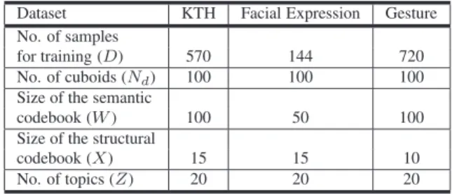
cuboids. K-means clustering is done on all cuboids from videos in a training set based on their appearance w and locationxand then semantic and structural codebooks are formed from the cluster centres. Vector quantitisation is then performed on all cuboids so that each of them is quan-titised into one of the (W×X) code-words. Co-occurrence matrix of size(W ×X)×D (whereD is the number of videos for training) is then formed by concatenating cuboid histograms (each with size(W×X)×1) of videos in the training set. The co-occurrence matrix can be served as an input of the pLSA algorithms (with the number of itera-tion set to 100) described in the previous secitera-tion and pLSA model parameters, P(z|d)andP((w, x)|z), can be learnt for testing. In our experiments, the number of topic, Z, was set slightly larger than the number of motion category involved (around 10). The motion class,t, can be inferred from the topic reported usingP(t|z)which can be estimated by counting the occurrence of topics and motion classes in the training set.
3. Experiments
3.1. Datasets
We conducted experiments in three different domains, namely human activity, facial expression and hand gesture.
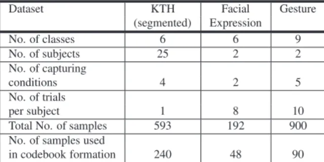
The human activity dataset (KTH dataset1) was introduced by Schuldt et al. [12], the facial expression dataset was col-lected by Doll´ar et al. [3] and the hand gesture dataset was captured by us. Table 1 summarises the details of them and Figure 3 shows samples from them. We performed leave-one-out cross-validation to evaluate our algorithm so that videos from a certain subject under a certain condition were used in testing and the remaining were used in training. The result is reported as the average of all possible runs.
Dataset KTH Facial Gesture
(segmented) Expression
No. of classes 6 6 9
No. of subjects 25 2 2
No. of capturing
conditions 4 2 5
No. of trials
per subject 1 8 10
Total No. of samples 593 192 900
No. of samples used
in codebook formation 240 48 90
Table 1. Details of the dataset used in our experiments.
(a) KTH
Anger Digust Fear
joy sadness surprise
(b) Facial Expression
(c) Gesture
Figure 3. Sample images in the three datasets used.
1The original KTH dataset was processed such that actions presented in
it are aligned and there is one iteration of action per sample. We refer the original dataset as unsegmented KTH and the processed one as segmented KTH.
3.2. Algorithms for Comparison
Since the experimental setting (e.g. the size of training sets) of previous studies such as [12, 11] are not the same as ours and the results cannot be compared directly, thus, we ran our implementations of their methods using a unified setting. The setting used was obtained empirically such that the recognition rate of standard pLSA is maximised. The code was written in Matlab running in a P4 1GB memory computer. Table 2 and 3 summarise the algorithms and the setting used respectively. The recognition algorithm using Support Vector Machines (SVM) was implemented based on Schuldt et al. work [12], with a replacement of its local kernel by a radial kernel on histogram inputs so that both SVM and pLSA models used the same input.
Algorithm Description
pLSA pLSA applied on (w) histogram
ABS-pLSA ABS-pLSA applied on (w, xabs) histogram TSI-pLSA TSI-pLSA applied on (w, xrel) histogram pLSA-ISM our pLSA-ISM applied on (w, xrel) histogram W-SVM SVM applied on (w) histogram
WX-SVM SVM applied on (w, xrel) histogram
Table 2. Details of the algorithms used in our experiments.
Dataset KTH Facial Expression Gesture
No. of samples
for training (D) 570 144 720
No. of cuboids (Nd) 100 100 100
Size of the semantic
codebook (W) 100 50 100
Size of the structural
codebook (X) 15 15 10
No. of topics (Z) 20 20 20
Table 3. The pLSA setting used in our experiments.
3.3. Results
3.3.1 Recognition
Since video samples from all three datasets used are well segmented, there is only small difference in perfor-mance between ABS-pLSA, TSI-pLSA and our pLSA-ISM. Therefore, we show only experimental results on recognition obtained from pLSA, pLSA-ISM, W-SVM and WX-SVM. The results are summarised in Table 4 and the confusion matrices obtained by our method pLSA-ISM are given in Figure 4.
From experiments, we can observe that structural infor-mation plays an important role in improving recognition accuracy (note that the accuracy obtained by WX-SVM is higher than that obtained by W-SVM, and similarly pLSA-ISM works better than pLSA). It is also found that the SVMs used scored better than the pLSA algorithms. How-ever, SVMs require labelled data as an input while the pLSA models can learn categories in an unsupervised manner.
pLSA W-SVM pLSA-ISM WX-SVM
KTH:
- Accuracy(%) 68.53 78.21 83.92 91.6
- Training time (s) 82.20 1.84 1.4e+3 3.59
- Testing time (s) 0.25 0.17 5.48 0.25
Facial Expression:
- Accuracy(%) 50.00 62.04 83.33 88.54
- Training time (s) 9.90 0.21 175.54 0.29
- Testing time (s) 0.62 0.08 7.98 0.12
Gesture:
- Accuracy(%) 76.94 86.13 91.94 97.78
- Training time (s) 121.06 3.18 1.2e+3 5.39
- Testing time (s) 8.20 0.27 47.25 1.32
Table 4. Comparison between recognition results obtained from pLSA, pLSA-ISM and SVMs.
(a) KTH (b) Facial Expression (c) Gesture Figure 4. Confusion matrices generated by applying pLSA-ISM on three datasets used.
3.3.2 Localisation
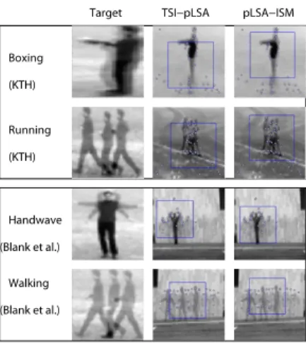
To compare the performance between ABS-pLSA, TSI-pLSA and TSI-pLSA-ISM, we evaluated them using unseg-mented KTH dataset (with unknown centroid location) and tested whether they could localise the occurrence of a mo-tion and recognise the momo-tion. We also exploited the human motion data used by Blank et al. [1] for giving some quali-tative results (Their data shares only 3 motion classes with KTH and there are only 10 sequences per class which is not sufficient for a quantitative test).
Quantitative test was done on unsegmented KTH dataset using the classifiers learnt in the previous experiment. Ta-ble 5 summarises the results obtained from ABS-pLSA, TSI-pLSA and pLSA-ISM. Some qualitative test results on both unsegmented KTH data and sequences from Blank et al. are shown in Figure 5.
ABS-pLSA TSI-pLSA pLSA-ISM KTH DB:
- Accuracy(%) 41.55 61.27 71.83
- Testing time (s) 9.64 9.81 9.78
Table 5. Comparison between recognition results obtained from ABS-pLSA, TSI-pLSA and pLSA-ISM.
We can observe from this experiment that our pLSA-ISM works better than the other two pLSA algorithms. The reason may be our method provides a stronger prior on centroid locations whose association with the semantic of
Figure 5. Localisation result on KTH dataset and sequences from Blank et al. using TSI-pLSA and pLSA-ISM.
cuboids has been learnt while TSI-pLSA assumes uniform distribution of centroid locations.
3.3.3 Retraining
We conducted this experiment to evaluate the performance of our retraining algorithm. KTH dataset was exploited in this experiment. The setting for training pLSA-ISM was the same as the one shown in Table 3, and we used leave-one-out cross validation (testing on segmented KTH data). Different from the first experiment, we varied the number of samples for training (we will use ‘number of subjects’ to describe the amount of data later and there are around 24 samples associated with each subject). In control set-up, we provided centroid locations (i.e. using segmented KTH data) for batch training. In test set-up, we used unsegmented KTH data for incremental training (i.e. retrain an initial model with a certain amount of new unsegmented data).
Firstly, the control set-up was used to determine the min-imum amount of data to obtain a pLSA-ISM model with an acceptable performance (e.g. over 70% accuracy), and eventually 5 subjects was used to obtain an initial model. Then in the test set-up, we re-trained the initial model with various amount of data. The result is shown in Table 6.
Total number of subjects used (prop. to sample size)
1 5 10 15 20 24
Control set-up 67.46 73.80 77.50 80.37 81.67 83.92
Test set-up N/A N/A 77.32 78.03 77.32 82.07
Table 6. The accuracy (%) obtained by pLSA-ISM through re-training is shown. Control set-up involves batch re-training using segmented KTH data (24 samples associated with 1 subject) while test set-up involves retraining of an initial model (built from 5 jects) using unsegmented samples. Note that if the number of sub-ject is shown as 10, this means a batch of 10×24 samples was used in training in the control set-up while there was a batch of 5×24 samples was added to retrain the initial model in the test set-up.
The result shows that pLSA-ISM can be retrained by unsegmented data to achieve a similar accuracy as if seg-mented data was used. Besides, pLSA-ISM needs only 5 subjects (120 samples) to achieve accuracy over 70% while WX-SVM needed more than 15 subjects to achieve the same accuracy according to our experience. This indicates another advantage of our unsupervised model over SVM.
4. Conclusion
This paper introduces a novel generative part-based model which extends pLSA to capture both semantic (content of parts) and structural (connection between parts) information for learning motion categories. Experimental results show that our model can improve recognition accuracy by using structural cues and it performs better in motion localisation than other pLSA models support-ing structural information. Although our model usually requires a set of training samples with known centroid locations, a retraining algorithm is introduced to accept samples with unknown centroids so that we can reduce the amount of human intervention in model reinforcement. Acknowledgements. SW is funded by the Croucher Foundation and TK is supported by the Toshiba and the Chevening Scholarship.
References
[1] M. Blank, L. Gorelick, E. Shechtman, M. Irani, and R. Basri. Actions as space-time shapes. InProc. ICCV, pages 1395–1402, 2005. [2] O. Boiman and M. Irani. Detecting irregularities in images and in
video. InProc. ICCV, pages 462–469, 2005.
[3] P. Doll´ar, V. Rabaud, G. Cottrell, and S. Belongie. Behavior recog-nition via sparse spatio-temporal features. InICCV Workshop: VS-PETS, 2005.
[4] A. A. Efros, A. C. Berg, G. Mori, and J. Malik. Recognizing action at a distance. InProc. ICCV, pages 726–733, 2003.
[5] C. Fanti, L. Zelnik-Manor, and P. Perona. Hybrid models for human motion recognition. InProc. CVPR, pages 1166–1173, 2005. [6] R. Fergus, L. Fei-Fei, P. Perona, and A. Zisserman. Learning object
categories from google’s image search. InProc. ICCV, 2005. [7] T. Hofmann. Unsupervised learning by probabilistic latent semantic
analysis.Machine Learning, 42(1-2):177–196, 2001.
[8] Y. Ke, R. Sukthankar, and M. Hebert. Efficient visual event detection using volumetric features. InProc. ICCV, pages 166–173, 2005. [9] I. Laptev. On space-time interest points. IJCV, 64(2-3):107–123,
2005.
[10] B. Leibe, E. Seemann, and B. Schiele. Pedestrian detection in crowded scenes. InProc. CVPR, pages 878–885, 2005.
[11] J. C. Niebles, H. Wang, and L. Fei-Fei. Unsupervised learning of hu-man action categories using spatial-temporal words. InProc. BMVC, 2006.
[12] C. Schuldt, I. Laptev, and B. Caputo. Recognizing human actions: A local svm approach. InProc. ICPR, 2004.
[13] E. Shechtman and M. Irani. Space-time behavior based correlation. InProc. CVPR, pages 405–412, 2005.
[14] J. Sivic, B. Russell, A. A. Efros, A. Zisserman, and B. Freeman. Discovering objects and their location in images. InProc. ICCV, 2005.
[15] Y. Song, L. Goncalves, and P. Perona. Unsupervised learning of human motion.PAMI, 25:814–827, 2003.
[16] A. Yilmaz and M. Shah. Recognizing human actions in videos ac-quired by uncalibrated moving cameras. InProc. ICCV, 2005.