The Chinese Restaurant Process

COS 597C: Bayesian nonparametrics

Lecturer: David Blei Lecture # 1

Scribes: Peter Frazier, Indraneel Mukherjee September 21, 2007 In this first lecture, we begin by introducing the Chinese Restaurant Pro-cess. After a brief review of finite mixture models, we describe the Chinese Restaurant Process mixture, where the latent variables are distributed ac-cording to a Chinese Restaurant Process. We end by noting a connection between Dirchlet processes and the Chinese Restaurant Process mixture.

The Chinese Restaurant Process

We will define a distribution on the space of partitions of the positive integers,

N. This would induce a distribution on the partitions of the first n integers,

for every n ∈_N.

Imagine a restaurant with countably infinitely many tables, labelled 1,2, . . .. Customers walk in and sit down at some table. The tables are chosen ac-cording to the following random process.

1. The first customer always chooses the first table.

2. The nth customer chooses the first unoccupied table with probability α

n−1+α, and an occupied table with probability c

n−1+α, where c is the number of people sitting at that table.

In the above, α is a scalar parameter of the process. One might check that the above does define a probability distribution. Let us denote by kn the number of different tables occupied after n customers have walked in. Then 1 ≤ kn ≤ n and it follows from the above description that precisely tables 1, . . . , kn are occupied.

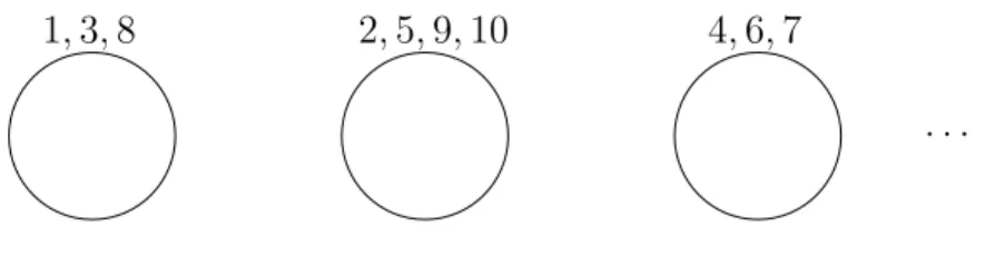
Example A possible arrangement of 10 customers is shown in Figure 1. Denote by zi the table occupied by the customer i. The probability of this arrangement is

1,3,8 2,5,9,10 4,6,7

. . .

Figure 1: The Chinese restaurant process. Circles represent tables and the numbers around them are the customers sitting at that table.

Pr(z1, . . . , z10) = Pr(z1) Pr(z2|z1). . .Pr(z10|z1, . . . , z9)

= α

α α

1 +α

1 2 +α

α

3 +α

1 4 +α

1 5 +α

2 6 +α

2 7 +α

2 8 +α

3 9 +α

We can make the following observations:

1. The probability of a seating is invariant under permutations. Permut-ing the customers permutes the numerators in the above computation, while the denominators remains the same. This property is known as exchangeability.

2. Any seating arrangement creates a partition. For example, the above seating arrangement partitions customers 1, . . . ,10 into the following three groups (1,3,8),(2,5,9,10),(4,6,7). Exchangeability now implies that two seating arrangements whose partitions consist of the same number of components with identical sizes will have the same proba-bility. For instance, the probability of any seating arrangement of ten customers where three tables are occupied, with three customers each on two of the tables and the remaining four on the third table, will have the same probability as the seating in our example.

Thus we could define a distribution on the space of all partitions of the integer n, where n is the total number of customers. The number of partitions is given by the partition function p(n), which has no simple closed form. Asymptotically, p(n) = exp(O(√n)).

3. The expected number of occupied tables for n customers grows loga-rithmically. In particular

E[kn|α] =O(αlogn)

This can be seen as follows: Let Xi be the IRV for the event that the

i th customer starts a new table. The probability of this happening is Pr[Xi = 1] =α/(i−1+α). Sincekn=P_iXi, by linearity of expectatin the summation is equal toP

iα/(α+i−1) which is upper bounded by

O(αHn) where Hn is the nth harmonic sum.

By taking the limit as n goes to infinity, we could perhaps define a dis-tribution on the space of all natural numbers. However, technical difficulties might arise while dealing with distributions over infinite sequences, and ap-propriate sigma algebras have to be chosen. Chapters 1-4 of [5], and the lecture notes from ORFE 551 (sent to course mailing list) are recommended for reading up basic measure theory.

Review: Finite mixture models

Finite mixture models are latent variable models. To model data via finite mixtures of distributions, the basic steps are

1. Posit hidden random variables

2. Construct a joint distribution of observed and hidden random variables 3. Compute the posterior distribution of the hidden variables given the

observed variables.

Examples include Gaussian mixtures, Kalman filter, Factor analysis, Hid-den Markov models, etc. We review the Gaussian mixture model.

A Gaussian mixture with K components, for fixed K, can be described by the following generative process:

1. Choose cluster proportionsπ∼Dir(α), whereDir(α) is a dirichlet prior, with parameter α, over distributions over k points.

3. For each data point:

(a) Choose cluster assignmentz ∼Mult(π) (b) Choose x∼N(µz, σX2).

The above gives a model for the joint distribution Pr(π, µ1:K, z1:Nx1:N|α, σµ2, σ2X). We will drop α, σ2

µ, σ2X from now on, and assume they are known and fixed. The posterior distribution, given data x1:N is Pr(π, µ1:K, z1:N|x1:N) and has the followin:

1. This decomposed the data over the latent space, thus revealing under-lying structure when present.

2. The posterior helps predict a new data point via thepredictive distribu-tion Pr(x|x1:N). For simplicity, we show how to calculate this quantity when the cluster proportions π is fixed.

Pr(x|x1:N, π) = X

z Z

µz

Pr(x, z, µz|x1:N, π)dµz

= X

z Z

µz

πzPr(x|µz) Pr(µz|x1:N)dµz

= X

z

πz Z

µz

Pr(x|µz) Pr(µz|x1:N)dµz

We could compute Pr(µz|x1:N)dµzfrom the posterior Pr(µ1:K, z1:N|x1:N, π) by marginalizing out thez1:N and the µk for k6=z. This would enable us to complete the above calculation to obtain the predictive distribu-tion.

Chinese Restaurant Process Mixture

A Chinese restaurant process mixture is constructed by the following proce-dure:

1. Endow each table with a mean,µ∗_k∼N(0, σ2

µ), k= 1,2, . . .. 2a. Customer n sits down at table zn∼CRP(α;z1, . . . , zn−1).

µ∗₁

1,3,8

µ∗₂

2,5,9,10

µ∗₃

4,6,7

. . .

Figure 2: The Chinese restaurant process mixture. Each table k has a mean

µ∗_kand customers sitting at it are distributed according to that mean. Tables 1 through 3 and customers 1 through 10 are pictured.

2b. A datapoint is drawn xn∼N(µ∗zn, σ

2

x).

We will consider the posterior and predictive distributions. The hidden variables are the infinite collection of means, µ∗₁, µ∗₂, . . ., and the cluster as-signments z1, z2, . . .. Consider the posterior on these hidden variables given

the first N datapoints,

p(µ∗_1:N, z1:N |x1:N, θ), where we defineθ = (σ2

µ, σ2x, α) to contain the fixed parameters of the model. Note that we only need to care about the means of the firstN tables because the rest will have posterior distribution N(0, σ2_µ) unchanged from the prior. Similarly, we only need to care about the cluser assignments of the first N

customers because the rest will have posterior equal to the prior.

The predictive distribution given the data and some additional hidden variables is

p(x|x1:N, µ∗1:N+1, z1:N, θ) =

1+KN

X

z=1

p(z |z1:N)p(x|z, µ∗z).

These hidden variables may be integrated out with the posterior on the hid-den variables to give the predictive distribution conditioned only on the data. Note that, whereas in the finite mixture model the cluster proportions were modeled explicitly, here the cluster proportions are within the z variables. Also note that permuting thex1:N results in the same predictive distribution, so we have exchangeability here as we did earlier.

Why is exchangeability important? Having exchangeability is as though we drew a parameter from a prior and then drew data independently and

identically from that prior. Thus, the data are independent conditioned on the parameter, but are not independent in general. This is weaker than assuming independence.

Specifically, DeFinetti’s exchangeability theorem [1] states that the ex-changeability of a random sequence x1, x2, . . . is equivalent to having a

pa-rameter θ drawn from a distribution F(·) and then choosing xn iid from the distribution implied by θ. That is,

θ ∼F(·)

xn iid

∼ θ.

We may apply this idea to the Chinese restaurant process mixture, which is really a distribution on distributions, or a distribution on the (µz1, µz2, . . .). The random means µz1, µz2, . . . are exchangeable, so this implies that their distribution may be expressed in the form given by DeFinetti’s exchangeabil-ity theorem. Their distribution is given by

G∼DirichletProcess(αG0) µzi

iid

∼G.

Here G0 is the distribution of the µ∗ on the reals, e.g., N(0, σ_u2). Note that we get repeated values when sampling the zi whenever a customer sits at an already occupied table. Then customer ihas µzi identical to theµzj of

all customers j previously seated at the table. In fact, G is an almost surely discrete distribution on the reals with a countably infinite number of atoms. The reading for next week, [2, 4], is on how to compute the posterior of the hidden parameters given the data, and also includes two new perspectives on the Chinese restaurant process. One perspective is the one just described, of the Chinese restaurant process as a Dirichlet process, and the other is as an infinite limit of finite mixture models. In the reading, focus on [4]. In addition, a good general reference on Bayesian statistics that may be helpful in the course is [3].

References

[1] Jose-M. Bernardo and Adrian F. M. Smith. Bayesian theory. Wiley Series in Probability and Mathematical Statistics: Probability and Mathemati-cal Statistics. John Wiley & Sons Ltd., Chichester, 1994.

[2] Michael D. Escobar and Mike West. Bayesian density estimation and in-ference using mixtures. J. Amer. Statist. Assoc., 90(430):577–588, 1995. [3] Andrew Gelman, John B. Carlin, Hal S. Stern, and Donald B. Rubin.

Bayesian data analysis. Texts in Statistical Science Series. Chapman & Hall/CRC, Boca Raton, FL, second edition, 2004.

[4] Radford M. Neal. Markov chain sampling methods for Dirichlet process mixture models. J. Comput. Graph. Statist., 9(2):249–265, 2000.

[5] David Williams. Probability with martingales. Cambridge Mathematical Textbooks. Cambridge University Press, Cambridge, 1991.