Worst-Case Conditional Value-at-Risk with
Application to Robust Portfolio
Management
Shu-Shang ZhuDepartment of Management Science, School of Management, Fudan University, Shanghai 200433, China, [email protected]
Masao Fukushima
Department of Applied Mathematics and Physics, Graduate School of Informatics, Kyoto University, Kyoto 606-8501, Japan, [email protected]
(Original version: July 5, 2005; Revised version: June 23, 2006)
This paper considers the worst-case CVaR in situation where only partial information on the underlying probability distribution is given. It is shown that, like CVaR, worst-case CVaR remains a coherent risk measure. The minimization of worst-case CVaR under mix-ture distribution uncertainty, box uncertainty and ellipsoidal uncertainty are investigated. The application of worst-case CVaR to robust portfolio optimization is proposed, and the corresponding problems are cast as linear programs and second-order cone programs which can be efficiently solved. Market data simulation and Monte Carlo simulation examples are presented to illustrate the methods. Our approaches can be applied in many situations, including those outside of financial risk management.
Subject Classifications: Finance, portfolio: conditional VaR, portfolio optimization; Pro-gramming, linear, nonlinear: robust optimization, second-order cone programming.
1
Introduction
Generally, two types of decision making frameworks are adopted in financial optimization: the utility maximization and the return-risk off analysis. In the return-risk trade-off analysis, the risk is explicitly quantified by a risk measure that maps the loss to a real number. Since it facilitates the understanding of risk, this approach is widely adopted in both practical applications and theoretical study. Although the utility maximization exhibits some theoretical elegance, it describes the risk in an indirect way, and consequently is rarely adopted in practice.
Markowitz (1952) paved the foundation for modern portfolio theory. His mean-variance analysis is a representative methodology in the framework of return-risk trade-off analysis, where variance is adopted as the measure of risk. Since the middle of 1990s, Value-at-Risk
(VaR, see RiskMetricsTM 1996), a new measure of downside risk, has become popular in
financial risk management. It has even been recommended as a standard on banking super-vision by Basel Committee. However, VaR has been criticized in recent years, especially in three aspects. First, VaR is not sub-additive in the general distribution case, consequently it is not a coherent risk measure in the sense of Artzner et al. (1999). Next, as a function of the portfolio positions, VaR may exhibit multiple local extrema for discrete distributions. Therefore VaR is hard to be optimized in this case. Finally, VaR is just a percentile of a probability distribution, and it does not fully grasp the information of the uncertainty beyond itself. Philippe (1996) presents some details of risk management using VaR. One can find plenty of materials on the theory, modeling, algorithms, and applications related to VaR at http://www.gloriamundi.org which is updated on-line.
Conditional Value-at-Risk (CVaR), defined as the mean of the tail distribution exceeding VaR, has attracted much attention in recent years. As a measure of risk, CVaR exhibits some better properties than VaR. Rockafellar and Uryasev (2000, 2002) showed that minimizing CVaR can be achieved by minimizing a more tractable auxiliary function without predetermin-ing the correspondpredetermin-ing VaR first, and at the same time, VaR can be calculated as a by-product. The CVaR minimization formulation given by Rockafellar and Uryasev (2000, 2002) usually results in convex programs, and even linear programs. Thus, their work opened the door to applying CVaR to financial optimization and risk management in practice. Pflug (2000) and Acerbi and Tasche (2002) proved that CVaR is a coherent risk measure. Rockafellar and Uryasev (2002) further explained the coherence of CVaR, and showed that CVaR is stable in the sense of continuity with respect to the confidence levelβ. Pflug (2000) and Ogryczak and Ruszczy´nski (2002) showed that CVaR is in harmony with the stochastic dominance princi-ples which are closely related to the utility theory. Konno, Waki and Yuuki (2002) illustrated the significance of using CVaR in reducing downside risk in portfolio optimization. All these stimulate the application of CVaR in practice. It is evidenced that CVaR is becoming more and more popular in financial management (Andersson et al. 2001, Bogentoft, Romeijn and Uryasev 2001, Topaloglou, Vladimirou and Zenios 2002).
As pointed out by Black and Litterman (1992), for the classical mean-variance model, the portfolio decision is very sensitive to the mean and the covariance matrix, especially to the mean. They showed that a small change in the mean can produce a large change in the optimal portfolio position. Thus the modeling risk arises due to the uncertainty of the underlying probability distribution. The uncertainty of the distribution can readily be observed in the case where enough data samples are not available, or the data samples are unstable. Moreover, it occurs in many other situations, such as portfolio selection with uncertain time of exit (Martellini and Uroˇsevi´o 2005). Another typical example is the decentralized investment management system (Mulvey and Erkan 2003), where each decision maker might have personal views on the future markets and cannot agree with each other.
Ben-Tal, Margalit and Nemirovski (1999) formulated a robust multi-stage portfolio problem using a robust linear programming approach. Lobo and Boyd (2000), Costa and Paiva (2002), Goldfarb and Iyengar (2003) studied the robust portfolio in the mean-variance framework. Instead of the precise information on the mean and the covariance matrix of asset returns, they introduced some types of uncertainties, such as polytopic uncertainty, box uncertainty and ellipsoidal uncertainty, in the parameters involved in the mean and the covariance matrix, and then translated the problem into semidefinite programs or second-order cone programs, which can efficiently be solved by interior-point algorithms developed in recent years. Halld´orsson and T¨ut¨unc¨u (2003) applied their interior-point method for saddle-point problems to the robust mean-variance portfolio selection under the box uncertainty in the elements of the mean vector and the covariance matrix. El Ghaoui, Oks and Oustry (2003) investigated the robust portfolio optimization using worst-case VaR, where only partial information on the distribution is known. Several formulations corresponding to various partial information structures have extensively been exploited to formulate the problems as semidefinite programs. Goldfarb and Iyengar (2003) also considered the robust VaR portfolio selection problem by assuming a normal distribution.
Robust optimization is not a new field in operations research. However, it is the break-through of the research in conic programming that has greatly stimulated the state-of-the-art of the robust optimization. The reader interested in robust optimization is referred to Ben-Tal and Nemirovski (2002) and the references therein.
In this paper, we consider the worst-case CVaR in situation where the information on the underlying probability distribution is not exactly known. The paper is outlined as follows: In the next section, we introduce the concept of worst-case CVaR and show that it remains coherent. We focus on, in this section, investigating the minimization of worst-case CVaR associated with mixture distribution uncertainty, box uncertainty and ellipsoidal uncertainty in the distributions. In Section 3, we present the application of worst-case CVaR to robust portfolio optimization, together with some illustrative numerical examples. Finally, we give some concluding remarks and discuss some future directions in this topic in Section 4.
2
Minimization of Worst-Case CVaR
Let f(x,y) denote the loss associated with decision vector x ∈ X ⊆ Rn and random vector y ∈ Rm (We use boldface letters to denote vectors and capital letters to denote matrices).
For the sake of simple formulation and clear understanding, we assume that y follows a continuous distribution in the first part of this section, and denote its density function asp(·). However all the results remain true for general distributions (see Remark 1). We also assume E(|f(x,y)|) < +∞ for each x ∈ X, so that CVaR and worst-case CVaR will be properly defined.
repre-sented as
Ψ(x, α),
Z
f(x,y)≤α
p(y)dy.
Given a confidence level β (usually greater than 0.9) and a fixed x ∈ X, the value-at-risk is defined as
VaRβ(x),min{α∈ R: Ψ(x, α)≥β}.
The corresponding conditional value-at-risk, denoted by CVaRβ(x), is defined as the expected
value of loss that exceeds VaRβ(x), that is, CVaRβ(x), 1
1−β
Z
f(x,y)≥VaRβ(x)
f(x,y)p(y)dy.
Rockafellar and Uryasev (2000, 2002) demonstrate that the calculation of CVaR can be achieved by minimizing the following auxiliary function with respect to variable α∈ R:
Fβ(x, α),α+1−1β
Z
y∈Rm
[f(x,y)−α]+p(y)dy, (1) where [t]+= max{t,0}. Thus we have the formula
CVaRβ(x) = min
α∈RFβ(x, α). (2)
Instead of assuming the precise knowledge of the distribution of random vector y, we assume in this paper that the density function is only known to belong to a certain setP of distributions, i.e.,
p(·)∈P.
Definition 1 The worst-case CVaR (WCVaR) for fixed x ∈ X with respect to P is
defined as
WCVaRβ(x), sup p(·)∈P
CVaRβ(x). (3)
As to the worst-case CVaR, one interesting question should be asked: Does the worst-case CVaR remain a coherent risk measure? We answer the question in the following. Motivated by characterizing the rationale of risk measure, Artzner et al. (1999) presented their seminal work on coherent risk measure. They advocated the following set of consistency rules for a risk measureρ mapping random loss X to a real number:
(i) Subadditivity: for all random losses X and Y,ρ(X+Y)≤ρ(X) +ρ(Y); (ii) Positive homogeneity: for positive constantλ,ρ(λX) =λρ(X);
(iii) Monotonicity: ifX ≤Y for each outcome, thenρ(X)≤ρ(Y); (iv) Translation invariance: for constantm,ρ(X+m) =ρ(X) +m.
A risk measure that satisfies the above four desirable axioms is called a coherent risk measure. Usually, random loss X is defined on some probability space (Ω,F, P) with a crisp (or determinate) probability measure P. In the situation thatP is ambiguous and characterized as a certain setP, then we can generally define the worst-case risk measureρw related toρ as
follows:
ρw(X),sup P∈P
ρ(X).
The following proposition claims that worst-case CVaR is still a coherent risk measure since CVaR is a coherent risk measure.
Proposition 1 Ifρassociated with crisp probability measureP is a coherent risk measure,
then the correspondingρw associated with ambiguous probability measurePremains a coherent
risk measure.
Proof. (i) Subadditivity: ρw(X+Y) = sup
P∈P
ρ(X+Y) ≤ sup
P∈P
[ρ(X) +ρ(Y)] ≤ sup
P∈P
ρ(X) + sup
P∈P
ρ(Y) = ρw(X) +ρw(Y); (ii) Positive homogeneity: for positive constant λ, ρw(λX) =
sup
P∈P
ρ(λX) = sup
P∈P
λρ(X) = λsup
P∈P
ρ(X) = λρw(X); (iii) Monotonicity: if X ≤ Y for each
outcome ω ∈Ω, then ρ(X) ≤ ρ(Y) for any given probability measure P ∈ P, which implies that ρw(X) = sup
P∈P
ρ(X) ≤ sup
P∈P
ρ(Y) = ρw(Y); (iv) Translation invariance: for constant m,
sup
P∈P
ρ(X+m) = sup
P∈P
[ρ(X) +m] = sup
P∈P
ρ(X) +m=ρw(X) +m. This completes the proof. ¤
In the rest of this section, with respect to worst-case CVaR, we will make further investi-gations on some special cases of P that meet practical requirements and, at the same time, the resulting problems can be efficiently solved. First we need to quote the following lemma which will serve as a key to transform the problem to a tractable one.
Lemma 1 Suppose X and Y are nonempty compact convex sets inRn and Rm,
respec-tively, and the functionφ(x,y)is convex inxfor any giveny, and concave iny for any given
x. Then we have
min
x∈Xmaxy∈Y φ(x,y) = maxy∈Y minx∈Xφ(x,y).
One can find the detail of this lemma in Fan (1953) and Bazaraa, Sherali and Shetty (1993, Chapter 6).
2.1 Mixture Distribution
We assume in this subsection that the distribution of y is only known to belong to a set of distributions which consists of all the mixtures of some predetermined likelihood distributions, i.e.,
p(·)∈PM ,
(
l
X
i=1
λipi(·) :
l
X
i=1
λi = 1, λi≥0, i= 1,· · · , l
)
, (4)
wherepi(·) denotes thei-th likelihood distribution, andldenotes the number of the likelihood
distributions. Mixture distribution has already been studied in robust statistics and used in modeling the distribution of financial data (Hall, Brorsen and Irwin 1989, Peel and McLachlan 2000). Denote
Λ,
(
λ= (λ1,· · · , λl) :
l
X
i=1
λi = 1, λi ≥0, i= 1,· · · , l
)
. (5)
Define
Fβi(x, α),α+ 1 1−β
Z
y∈Rm
[f(x,y)−α]+pi(y)dy, i= 1,· · ·, l.
Theorem 1 For each x, WCVaRβ(x) with respect to PM is given by
WCVaRβ(x) = min
α∈Rmaxi∈L F
i
β(x, α), (6)
where L,{1,2,· · · , l}.
Proof. For givenx∈ X, define
Hβ(x, α,λ) , α+1−1β
Z
y∈Rm
[f(x,y)−α]+
" l X
i=1
λipi(y)
# dy = l X i=1
λiFβi(x, α), (7)
whereλ∈Λ. Hβ(x, α,λ) is convex inα (see Rockafellar and Uryasev 2000, 2002) and affine
(concave) inλ. It is easy to see that minα∈RHβ(x, α,λ) is a continuous function with respect
toλ. By (2), (3), (4) and the fact that Λ is compact, we can write WCVaRβ(x) = max
λ∈Λαmin∈RHβ(x, α,λ) = maxλ∈Λminα∈R
l
X
i=1
λiFβi(x, α). (8)
For eachiand fixedx, the optimal solution set of minα∈RFβi(x, α) is a nonempty, closed
and bounded interval (see Rockafellar and Uryasev 2000, 2002). Thus we can denote [α∗i, α∗i],argmin
α∈R
Supposeg1(t) andg2(t) are two convex functions defined onR, and the nonempty, closed and
bounded intervals £t∗
1, t∗1
¤
,£t∗
2, t∗2
¤
are the sets of minima of these two functions, respectively. It can be easily verified that for anyβ1 ≥0 andβ2 ≥0 such thatβ1+β2 >0,β1g1(t)+β2g2(t)
is convex too, and the set of minima ofβ1g1(t) +β2g2(t) must lie in the nonempty, closed and
bounded interval£min{t∗
1, t∗2},max{t∗1, t∗2}
¤
. From this fact and (7), we get argmin
α∈R
Hβ(x, α,λ)⊆ A, ∀λ∈Λ, whereA is the nonempty, closed and bounded interval given by
A,
·
min
i∈L α ∗
i,maxi∈L α∗i
¸
. This implies
min
α∈RHβ(x, α,λ) = minα∈AHβ(x, α,λ).
Therefore, by Lemma 1, we have max
λ∈Λαmin∈RHβ(x, α,λ) = maxλ∈Λminα∈AHβ(x, α,λ) = minα∈Amaxλ∈ΛHβ(x, α,λ). (9)
It is obvious that
min
α∈Amaxλ∈ΛHβ(x, α,λ)≥αinf∈Rmaxλ∈ΛHβ(x, α,λ). (10)
By (9), (10) and the well known result on the min-max inequality inf
α∈Rmaxλ∈ΛHβ(x, α,λ)≥maxλ∈Λminα∈RHβ(x, α,λ),
we immediately get max
λ∈Λminα∈RHβ(x, α,λ) = minα∈Rmaxλ∈ΛHβ(x, α,λ).
It then follows from (8), along with (7) that WCVaRβ(x) = min
α∈Rmaxλ∈ΛHβ(x, α,λ) = minα∈Rmaxλ∈Λ l
X
i=1
λiFβi(x, α). (11)
Now we only need to verify the equivalence of the right-hand sides of (6) and (11). As an optimization problem, the right-hand side of (11) is equivalent to
min
(α,θ)∈R×R
(
θ:
l
X
i=1
λiFβi(x, α)≤θ,∀λ∈Λ
)
. (12)
From (5), it is clear that any feasible solution of (12) satisfies
On the other hand, if (13) holds, then for any λ∈Λ, we have
l
X
i=1
λiFβi(x, α)≤ l
X
i=1
λiθ=θ.
Thus problem (12) is equivalent to min
(α,θ)∈R×R
©
θ:Fβi(x, α)≤θ, i= 1,· · · , lª,
which is nothing but the right-hand side of (6). This completes the proof. ¤ Denote
FβL(x, α),max
i∈L F
i β(x, α).
By Theorem 1, we get the following corollary immediately.
Corollary 1 Minimizing WCVaRβ(x) over X can be achieved by minimizing FL
β(x, α)
over X × R, i.e.,
min
x∈XWCVaRβ(x) =(x,α)min∈X ×RF L
β(x, α).
More specifically, if(x∗, α∗)attains the right-hand side minimum, thenx∗ attains the left-hand
side minimum and α∗ attains the minimum of FβL(x∗, α), and vice versa.
It is known that Fβ(x, α) defined by (1) is convex in (x, α) if f(x,y) is convex in x (see
Rockafellar and Uryasev 2000, 2002). By the fact that the functiong(t) = max{g1(t), g2(t)}is
convex if bothg1(t) andg2(t) are convex, we get that iff(x,y) is convex inx, then FβL(x, α)
is convex in (x, α). So, if X is a convex set and f(x,y) is a convex function of x, then the WCVaR minimization problem is a convex program.
From now on, we discuss the computational aspect of minimization of WCVaR. Theorem 1 and Corollary 1 help us to translate the original problem to a more tractable one. It can be seen that the WCVaR minimization is equivalent to
min
(x,α,θ)∈X ×R×R
½
θ:α+ 1 1−β
Z
y∈Rm
[f(x,y)−α]+pi(y)dy≤θ, i= 1,· · ·, l
¾
. (14) The most difficult part in the computation of (14) is the calculation of the integral of a multivariate and non-smooth function. However, an approximation method can be used to deal with this difficulty. Monte Carlo simulation is one of the most efficient methods for high dimensional integral computation. Rockafellar and Uryasev (2000) use this method to approximate Fβ(x, α) as
˜
Fβ(x, α) =α+S(11−β) S
X
k=1
where y[k] denotes the k-th sample (We use the subscript [k] to distinguish a vector from a scalar) generated by simple random sampling with respect to y according to its density functionp(·), andSdenotes the number of samples. The Law of Large Numbers in probability theory guarantees the approximation accuracy (or convergence) when the number of samples becomes large enough. If f(x,y) is linear with respect to xand X is a convex polyhedron, then the Monte Carlo method produces linear programs, which can be efficiently solved.
Replacing the integral in (14) with (15) yields min
(x,α,θ)∈X ×R×R
θ:α+
1 Si(1−β)
Si
X
k=1
[f(x,yi[k])−α]+≤θ, i= 1,· · · , l
, (16)
where yi
[k] is the k-th sample with respect to the i-th likelihood distribution pi(·), and Si
denotes the number of corresponding samples. Instead of the simple random sampling method, some improved sampling approaches can be used to approximate the integral. Generally, the approximation of problem (14) can be formulated as
min
(x,α,θ)∈X ×R×R
θ:α+
1 1−β
Si
X
k=1
πki[f(x,y[k]i )−α]+≤θ, i= 1,· · · , l
, (17)
where πi
k denotes the probability according to thek-th sample with respect to the i-th
like-lihood distribution pi(·). If πi
k is equal to S1i for all k, then (17) reduces to (16). In the
following, we denote πi = ¡πi
1,· · ·, πiSi
¢T
. Then, by introducing an auxiliary vector u = (u1;u2;· · · ;ul)∈ Rmwherem=Pl
i=1Si, the optimization problem (17) can be reformulated
as the following tractable minimization problem with variables (x,u, α, θ)∈ Rn×Rm×R×R:
min θ (18)
s.t. x∈ X, (19)
α+ 1 1−β
¡
πi¢T ui ≤θ, i= 1,· · ·, l, (20)
uik≥f(x,y[k]i )−α, k= 1,· · · , Si, i= 1,· · ·, l, (21)
uik≥0, k= 1,· · · , Si, i= 1,· · ·, l. (22)
Furthermore, if f(x,y) is linear with respect to x and X is a convex polyhedron, then the problem can actually be solved via a linear programming approach.
Remark 1 In the special case where l= 1, i.e., the distribution of y is certainly known,
problem (18)-(22) is exactly that of Rockafellar and Uryasev (2000) with πki = S11 for all k.
Although in the above discussion we assume a continuous distribution, it is easy to see from Rockafellar and Uryasev (2002) that the results also hold in the general distribution case. For example, in the discrete distribution case, it is straightforward to interpret the integral as a summation. Moreover, it should be interpreted as a mixture of an integral and a summation in the case of mixed continuous and discrete distributions.
2.2 Discrete Distribution
In this subsection we assume thatyfollows a discrete distribution. From a practical viewpoint, this consideration still makes sense for continuous distributions in CVaR formulation, since we usually use a discretization procedure to approximate the integral resulting from a continuous distribution. Moreover, among various uncertainty structures, we are particularly interested in the minimization of worst-case CVaR under box uncertainty and ellipsoidal uncertainty. The reason for this choice is not only that these two types of uncertainty sets are the simplest ones to be specified, but also that the resulting problem can be formulated in a tractable way. Box uncertainty and ellipsoidal uncertainty, together with mixture distribution uncertainty, are the most often used uncertainty structures in robust optimization formulations (see, for example, Costa and Paiva 2002, Goldfarb and Iyengar 2003, Halld´orsson and T¨ut¨unc¨u 2003 and El Ghaoui, Oks and Oustry 2003).
Let the sample space of random vector ybe given by©y[1],y[2],· · ·,y[S]ªwith Pr©y[i]ª= πi and
PS
i=1πi = 1, πi ≥0, i= 1,· · · , S. Denote π= (π1, π2,· · · , πS)T and define
Gβ(x, α,π),α+
1 1−β
S
X
k=1
πk[f(x,y[k])−α]+.
For givenxandπ, the corresponding CVaR is then defined as (Rockafellar and Uryasev 2002) CVaRβ(x,π),min
α∈RGβ(x, α,π).
Especially, we denote P asPπ in the case of discrete distribution. Then we may identify
Pπ as a subset ofRS and the worst-case CVaR for fixedx∈ X with respect toPπ is defined
as
WCVaRβ(x), sup
π∈Pπ
CVaRβ(x,π),
or equivalently,
WCVaRβ(x), sup
π∈Pπ
min
α∈RGβ(x, α,π).
Theorem 2 Suppose Pπ is a compact convex set. Then, for each x, we have
WCVaRβ(x) = min
α∈Rπmax∈Pπ
Gβ(x, α,π).
Proof. Since Pπ is bounded, it is contained in a polytope, i.e.,
Pπ ⊆
(
π∈ RS: π=
l
X
i=1
λiπi, λ∈Λ
for some positive integer l and likelihood distributions {πi}l
i=1, where Λ is given by (5).
Therefore, for any given π ∈ Pπ, using a similar argument to that in the first part of
Theorem 1, we can show that min
α∈RGβ(x, α,π) = minα∈AGβ(x, α,π),
and hence
max π∈Pπ
min
α∈RGβ(x, α,π) = maxπ∈Pπ
min
α∈AGβ(x, α,π),
whereA is a nonempty, closed and bounded interval.
For fixed x, Gβ(x, α,π) is convex in α (see Rockafellar and Uryasev 2002) and affine
(concave) inπ. By Lemma 1, we get max
π∈Pπ
min
α∈AGβ(x, α,π) = minα∈Aπmax∈Pπ
Gβ(x, α,π).
Performing a further discussion similar to the proof of Theorem 1, we can show WCVaRβ(x) = min
α∈Rπmax∈Pπ
Gβ(x, α,π).
This completes the proof. ¤
Theorem 2 indicates that, if Pπ is a compact convex set, the problem of minimizing
WCVaRβ(x) over X can be equivalently formulated as the following minimization problem
with variables (x,u, α, θ)∈ Rn× RS× R × R:
min θ (23)
s.t. x∈ X, (24)
max π∈Pπ
α+ 1 1−βπ
Tu≤θ, (25)
uk ≥f(x,y[k])−α, k= 1,· · · , S, (26)
uk ≥0, k= 1,· · · , S. (27)
Problem (23)-(27) is not ready for application because of the max operation involved in the constraints. In the following, we show that, under box uncertainty and ellipsoidal uncertainty in the distributions, problem (23)-(27) can be cast as linear programs and second-order cone programs, respectively.
2.2.1 Box Uncertainty
Supposeπ belongs to a box, i.e.,
π∈PπB ,©π:π=π0+η,eTη= 0,η≤η≤ηª, (28)
where π0 is a nominal distribution which represents the most likely distribution, e denotes
π to be a probability distribution, and the non-negativity constraintπ ≥0 is included in the box constraints η≤η≤η.
Since
α+ 1 1−βπ
Tu=α+ 1
1−β
¡
π0¢T u+ 1 1−βη
Tu,
we have
max π∈PB
π
α+ 1 1−βπ
Tu=α+ 1
1−β
¡
π0¢T u+ γ
∗(u)
1−β, whereγ∗(u) is the optimal value of the following linear program
max η∈RS
©
uTη:eTη= 0,η≤η≤ηª. (29) The dual program of (29) is given by
min
(z,ξ,ω)∈R×RS×RS
©
ηTξ+ηTω:ez+ξ+ω=u,ξ≥0,ω≤0ª. (30)
Consider the following minimization problem over (x,u, z,ξ,ω, α, θ) ∈ Rn× RS× R ×
RS× RS× R × R:
min θ (31)
s.t. x∈ X, (32)
α+ 1 1−β
¡
π0¢Tu+ 1 1−β
¡
ηTξ+ηTω¢≤θ, (33)
ez+ξ+ω=u, (34)
ξ≥0, ω≤0, (35)
uk≥f(x,y[k])−α, k= 1,· · · , S, (36)
uk≥0, k= 1,· · ·, S. (37)
Proposition 2 If (x∗,u∗, z∗,ξ∗,ω∗, α∗, θ∗) solves (31)-(37), then (x∗,u∗, α∗, θ∗) solves
(23)-(27) with Pπ = PB
π; Conversely, if ( ˜x∗,u˜∗,α˜∗,θ˜∗) solves (23)-(27) with Pπ = PπB,
then ( ˜x∗,u˜∗,z˜∗,ξ˜∗,ω˜∗,α˜∗,θ˜∗) solves (31)-(37), where (˜z∗,ξ˜∗,ω˜∗) is an optimal solution to
(30) with u= ˜u∗.
Proof. Let (x∗,u∗, z∗,ξ∗,ω∗, α∗, θ∗) solve (31)-(37). Since (z∗, ξ∗, ω∗) is feasible to (30)
withu=u∗, by the duality theorem of linear programming, we have
Thus
max π∈PB
π
α∗+ 1 1−βπ
Tu∗
=α∗+ 1 1−β
¡
π0¢Tu∗+γ∗(u∗) 1−β
≤α∗+ 1
1−β
¡
π0¢Tu∗+ 1 1−β
¡
ηTξ∗+ηTω∗¢
≤θ∗,
which, together with constraints (32), (36), (37), implies that (x∗,u∗, α∗, θ∗) is feasible to
(23)-(27) withPπ =PπB.
Now assume (x∗,u∗, α∗, θ∗) is not an optimal solution to (23)-(27) with P
π =PπB, i.e.,
there exists an optimal solution ( ¯x∗,u¯∗,α¯∗,θ¯∗) to (23)-(27) such that
¯ θ∗ < θ∗.
Let (¯z∗,ξ¯∗,ω¯∗) be an optimal solution to (30) with u= ¯u∗. By the strong duality theorem
of linear programming, we have ¯
α∗+ 1 1−β
¡
π0¢T u¯∗+ 1 1−β
¡
ηTξ¯∗+ηTω¯∗¢ = ¯α∗+ 1
1−β
¡
π0¢T u¯∗+γ
∗( ¯u∗)
1−β = max
π∈PB π
¯
α∗+ 1 1−βπ
Tu¯∗
≤θ¯∗,
which, together with (24), (26), (27) and constraints in (30), implies that ( ¯x∗,u¯∗,z¯∗,ξ¯∗,ω¯∗,α¯∗,
¯
θ∗) is feasible to (31)-(37). This contradicts the assumption that (x∗,u∗, z∗,ξ∗,ω∗, α∗, θ∗) is
an optimal solution to (31)-(37) since ¯θ∗< θ∗. Thus (x∗,u∗, α∗, θ∗) is an optimal solution to
(23)-(27) withPπ =PπB.
Conversely, let ( ˜x∗,u˜∗,α˜∗,θ˜∗) solve (23)-(27) with P
π =PπB, and let (˜z∗,ξ˜∗,ω˜∗) denote
an optimal solution to (30) withu= ˜u∗. Then ( ˜x∗,u˜∗,z˜∗,ξ˜∗,ω˜∗,α˜∗,θ˜∗) must solve (31)-(37).
In fact, if this is not the case, then there exists an optimal solution (¯x∗,u¯∗,z¯∗,ξ¯∗,ω¯∗,α¯∗,θ¯∗) of
(31)-(37) such that ¯θ∗ <θ˜∗. From the discussion of the first part of the proof, ( ¯x∗,u¯∗,α¯∗,θ¯∗) is
an optimal solution of (23)-(27), which contradicts the assumption that ( ˜x∗,u˜∗,α˜∗,θ˜∗) solves
(23)-(27) since ¯θ∗ <θ˜∗. This completes the proof. ¤
Iff(x,y) is a convex function with respect toxandX is a convex set, then (31)-(37) is a convex program. Especially, iff(x,y) is linear inx and X is a convex polyhedron, then the problem is a linear program.
Remark 2 In the special case where η=η= 0, problem (31)-(37) reduces to the original
2.2.2 Ellipsoidal Uncertainty
Supposeπ belongs to an ellipsoid, i.e.,
π ∈PπE ,©π:π =π0+Aη,eTAη= 0,π0+Aη≥0,kηk ≤1ª, (38) wherekηk=pηTη,π0 is a nominal distribution that is the center of the ellipsoid,A∈ RS×S
is the scaling matrix of the ellipsoid. The conditions eTAη= 0 andπ0+Aη≥0 ensureπ to
be a probability distribution.
Consider the following convex program max
η∈RS
©
uTAη:eTAη= 0,π0+Aη≥0,kηk ≤1ª. (39) The dual of (39) is the second-order cone program
min
(ζ,ω,ξ,z)∈R×RS×RS×R
n
ζ+¡π0¢T ω:−ξ−ATω+ATez=ATu,kξk ≤ζ,ω≥0
o
. (40) One can refer to Lobo et al. (1998) and Alizadeh and Goldfarb (2003) for the details on second-order cone programming. Under some mild condition, such as the existence of inte-rior feasible points for both (39) and (40), the zero duality gap is guaranteed by the strong conic duality theorem. In this case, by using a similar argument to Proposition 2, we can equivalently formulate (23)-(27) withPπ =PE
π as the following minimization problem over
(x,u, ζ,ω,ξ, z, α, θ)∈ Rn× RS× R × RS× RS× R × R × R:
min θ (41)
s.t. x∈ X, (42)
α+ 1 1−β
¡
π0¢T u+ 1 1−β
h
ζ+¡π0¢T ω
i
≤θ, (43)
−ξ−ATω+ATez=ATu, (44)
kξk ≤ζ, ω≥0, (45)
uk≥f(x,y[k])−α, k= 1,· · · , S, (46)
uk≥0, k= 1,· · ·, S. (47)
If f(x,y) is a convex function with respect to x and X is a convex set, then problem (41)-(47) is a convex program. Furthermore, iff(x,y) is a linear function with respect to x
and X is a convex polyhedron, then the problem is a second-order cone program that can be solved efficiently by interior-point methods developed in recent years.
Remark 3 In the special case where A = 0, problem (41)-(47) reduces to the original
CVaR minimization problem.
2.3 Specification of Uncertainty Sets
How to determine the uncertainty sets in a reasonable way, more specifically, how to properly determine the likelihood distributions for mixture distribution uncertainty, the bounds for box
uncertainty and the scaling matrix for ellipsoidal uncertainty, is the key issue for successful practical applications. In this subsection we present some preliminary discussion on this issue. For mixture distibusion uncertainty, one way to specify the likelihood distributions is as follows: First, estimate the distribustion p(·, ψ) by historical data, where ψ denotes the dis-tribution parameters. Then determine the likelihood disdis-tributions p(·, ψi) (i = 1,· · · , l) by
properly choosing ψi ∈ Ψ, where Ψ denotes the confidence intervals of distribustion para-meters. Two alternative methods can be used in specifying likelihood distributions. One is historical simulation: a set of differently behaved historical data can be chosen as the samples of the likelihood distributions. The other is expert prediction: all the different distributions predicted by a group of experts can be chosen as the likelihood distributions for constructing mixture distributions.
To discuss the specification of uncertainty sets in the case of discrete distribution, we first assume that the nominal distributionπ0 ∈ RSand a set of possible distributionsπi∈ RS(i= 1,· · · , m) are known. With this information, the bounds of a box uncertainty set (28) can be chosen as
ηj = max
i∈{1,···,m}
©
π0j −πij,0ª and ηj = max
i∈{1,···,m}
©
πij−π0j,0ª, j= 1,· · ·, S.
Generally, for an ellipsoidal uncertainty set, it is a hard task to properly specify the scaling matrix A in (38). We consider here a special case: a ball uncertainty set, which means that the scaling matrix A is given by ρI, where I is the identity matrix and ρ is a nonnegative number to be specified. In this case, the ellipsoidal uncertainty set (38) reduces to the ball
©
π:kπ−π0k ≤ρª. Thusρ can be reasonably specified as
ρ= max
i∈{1,···,m}
©
kπi−π0kª.
It is clear that the larger the value of ρis, the more uncertain the distribution becomes. Finally, we should address that given partial information on the distribution, it is not hard to determine π0 and πi via scenario generation, such as moment matching approaches (see Høyland and Wallace (2001) and Ji et al. (2005)).
3
Robust Portfolio Management Using Worst-Case CVaR
In this section we consider the situation that random returns of financial assets are just specified by a set of distributions, and formulate a portfolio management problem by utilizing worst-case CVaR as the measure of risk.Suppose there existnrisk assets that can be chosen by the investor in the financial market. Let random vector y= (y1,· · · , yn)T ∈ Rn denote the uncertain returns of the nrisk assets,
by the investor. Thus the loss function is defined as f(x,y) =−xTy.
By definition, the portfolio return is the negative of the loss, i.e.,xTy.
Portfolio optimization tries to find an optimal trade-off between the risk and the return according to the investor’s preference, while the robust portfolio selection is performed through the worst-case analysis of risk and return. Thus the robust portfolio selection problem using WCVaR as a risk measure can be represented as
min
x∈XWCVaR(x),
whereX denotes the constraint on the portfolio position, which usually includes the require-ment of the worst case minimum expected return. According to the discussion in the previous section, in order to complete the formulation of the robust portfolio selection model, we only need to specify the constraint setX.
Suppose the investor has an initial wealth w0. Thus the portfolio satisfies
eTx=w0. (48)
To ensure diversification and satisfy the regulations, we impose the bound constraints on the portfolio
x≤x≤x, (49)
wherex andx are the given lower and upper bounds on the portfolios.
Let µ be the worst-case minimum expected return required by the investor. Mathemati-cally, this can be represented as
min
p(·)∈PEp
¡
xTy¢≥µ, (50)
where Epdenotes the expectation operator with respect to the distributionp(·) ofy. Generally,
X is specified by (48), (49) and (50), i.e.,
X ,
½
x:eTx=w0, x≤x≤x, min p(·)∈PEp
¡
xTy¢≥µ
¾
. (51)
3.1 Problem Formulations
In this subsection, we discuss robust portfolio selection problems corresponding to the three types of uncertainties described in the previous section. The problems are cast as linear programs and second-order programs.
3.1.1 Mixture Distribution Uncertainty
In the case of mixture distribution uncertainty given by (4), (50) can be written as
l
X
i=1
λiEpi
¡
xTy¢≥µ, ∀λ∈Λ, (52)
where Λ is defined by (5). It is easy to verify that (52) is equivalent to Epi
¡
xTy¢≥µ, i= 1,· · ·, l. (53)
Let ¯yi denote the expected value ofy with respect to likelihood distributionpi(·). Then (50)
can be simply represented as
xTy¯i≥µ, i= 1,· · · , l. (54)
By (18)-(22), the robust portfolio selection problem, under the mixture distribution situ-ation, is formulated as the following linear program with variables (x,u, α, θ)∈ Rn× Rm×
R × R:
min{θ: (20)-(22),(48),(49) and (54)}, (55) wheref(x,yi
[k]) in (21) should be particularly specified as−xTy[k]i .
3.1.2 Box Uncertainty in Discrete Distributions
Denote
Y =
y[1]T
.. .
yT [S]
. (56)
In the case of box uncertainty in discrete distributions, by (28) and (51), X is given by
XB ,
(
x: eTx=w0, x≤x≤x, (Yx)Tπ0+ min
{η:eTη=0,η≤η≤η}(Yx)
Tη≥µ
)
. The dual problem of the linear program
min η∈RS
©
(Yx)Tη:eTη= 0,η≤η≤ηª
is written as
max
(δ,τ,ν)∈R×RS×RS
©
ηTτ+ηTν :eδ+τ+ν =Yx,τ ≤0,ν ≥0ª. Define
ΦB ,
(
(x, δ,τ,ν) : e
Tx=w
0, x≤x≤x, eδ+τ+ν =Yx, τ ≤0, ν ≥0, (Yx)Tπ0+ηTτ +ηTν ≥µ
and
ΦBX ,©x:∃(δ,τ,ν) such that (x, δ,τ,ν)∈ΦBª. By the duality theory of linear programming, it is easy to see that
XB = ΦBX. (57)
By (31)-(37) and (57), the robust portfolio selection problem can be written as the following linear program with variables (x,u, z,ξ,ω, α, θ, δ,τ,ν)∈ Rn× RS× R × RS× RS× R × R ×
R × RS× RS:
min©θ: (33)-(37) and (x, δ,τ,ν)∈ΦBª, wheref(x,y[k]) in (36) should be particularly specified as−xTy[k].
3.1.3 Ellipsoidal Uncertainty in Discrete Distributions
In the case of the ellipsoidal uncertainty in discrete distributions, by (38) and (51),X is given by
XE ,
x:
eTx=w
0, x≤x≤x,
(Yx)Tπ0+ min
{η:eTAη=0,π0+Aη≥0,kηk≤1}(Yx)
TAη≥µ
,
whereY is defined by (56). The dual program of the second-order cone program min
η∈RS
©
(Yx)TAη:eTAη= 0,π0+Aη≥0,kηk ≤1ª. is given by
max
(σ,τ,ν,δ)∈R×RS×RS×R
n
−σ−¡π0¢T τ :ν+ATτ+ATeδ=ATYx,kνk ≤σ,τ ≥0
o
. Define
ΦE ,
(
(x, σ,τ,ν, δ) : e
Tx=w
0, x≤x≤x, ν+ATτ +ATeδ =ATYx,
kνk ≤σ, τ ≥0, (Yx)Tπ0−σ−¡π0¢T τ ≥µ
)
and
ΦEX ,©x:∃(σ,τ,ν, δ) such that (x, σ,τ,ν, δ)∈ΦEª.
By the conic duality theory, under some mild condition that guarantees zero duality gap, we have
XB = ΦEX. (58)
By (41)-(47) and (58), the robust portfolio selection problem can be written as the following second-order cone program with variables (x,u, ζ,ω,ξ, z, α, θ, σ,τ,ν, δ) ∈ Rn× RS × R ×
RS× RS× R × R × R × R × RS× RS× R:
min©θ: (43)-(47) and (x, σ,τ,ν, δ)∈ΦEª, (59) wheref(x,y[k]) in (46) should be particularly specified as−xTy
0 500 1000 1500 2000 2500 −0.2
−0.15 −0.1 −0.05 0 0.05 0.1 0.15 0.2
Day number of samples
Return
Period1 Period2 Period3
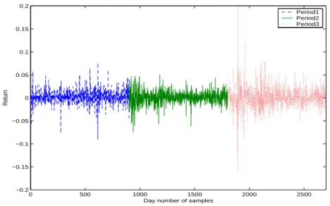
Figure 1: Return of Hang Seng Finance Index of SEHK (27/07/1990∼11/30/2000).
3.2 Numerical Examples
In this subsection, we consider two numerical examples to illustrate the robust portfolio optimization problems. Market data simulation analysis and Monte Carlo simulation analysis are presented.
3.2.1 Market Data Simulation Analysis
The four sectoral sub-indices of Hang Seng Index of Hong Kong Stock Exchange (SEHK): (1) Hang Seng Finance Index (HSNF), (2) Hang Seng Utilities Index (HSNU), (3) Hang Seng Property Index (HSNP), and (4) Hang Seng Commercial/Industrial Index (HSNC), are chosen as the financial assets to construct the portfolios. We consider the day returns of these assets in the example. 2700 samples of returns of these four assets are collected from the time period from July 27, 1990 to November 30, 2000. Figure 1 is constructed by the samples of day return of HSNF. The day returns of other three assets behave similarly to that of HSNF. It can be roughly observed from Figure 1 that the behaviour of returns is not consistent among different time periods. According to this observation, we divide the time period into the following three sub-intervals (900 samples for each time period):
• Period1: 07/27/1990 ∼01/06/1994;
• Period2: 01/07/1994 ∼06/19/1997;
• Period3: 06/20/1997 ∼11/30/2000.
Within each time period, the returns behave similarly, whereas they exhibit remarkable dif-ference between any two time periods.
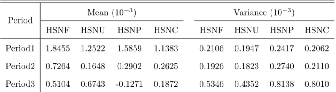
Table 1: Expected value and variance of returns of four indices in different time periods.
Period Mean (10
−3) Variance (10−3)
HSNF HSNU HSNP HSNC HSNF HSNU HSNP HSNC
Period1 1.8455 1.2522 1.5859 1.1383 0.2106 0.1947 0.2417 0.2062 Period2 0.7264 0.1648 0.2902 0.2625 0.1926 0.1823 0.2740 0.2110 Period3 0.5104 0.6743 -0.1271 0.1872 0.5346 0.4352 0.8138 0.8010
The expected values and variances of returns of the four assets corresponding to different time periods are listed in Table 1. We find that the expected return of Period1 and the volatility of Period3 are much larger than those of the other two time periods. In this example, the estimation of the statistical parameters is not stable. Thus it is questionable to assume that all the samples are generated by an identical nominal probability distribution. Consequently, the original CVaR, as the measure of risk, is not reliable if all those samples are used directly in calculation since the underlying assumption that the probability distribution is precisely known to be a nominal one is violated. In this situation, it is reasonable to assume a mixture distribution of the random returns, and it makes sense for us to perform a worst-case CVaR minimization.
In the example, according to our observation, we assume that the samples are generated by the mixture distribution of three likelihood distributions. The samples within each time period are assumed to be generated by the corresponding likelihood distribution.
SeduMi1.05 (Sturm 2001), a package developed by J. Sturm for optimization over symmet-ric cones, is employed in our computation. The numesymmet-rical experiments are implemented on PC (1.5G RAM, CPU 3.06GHz). All the problems are successfully solved within 10 seconds. Especially, the linear programs obtained from the the market data simulation analysis are always solved within 4 seconds.
In this example, we set β= 0.95, w0 = 1,x= (0,0,0,0)T and x= (1,1,1,1)T.Numerical
experiments for the nominal and the robust portfolio optimization problems are performed via the linear programming model (55). The former employs the original CVaR as the risk mea-sure, while the latter uses the worst-case CVaR. In the computation of the nominal portfolio optimization problem, we setl= 1 and S1= 2700, i.e., all the samples are used in the model
by assuming that they are generated by one nominal probability distribution. In the compu-tation of the robust portfolio optimization problem, we set l = 3 and S1 =S2 =S3 = 900, where we assume the samples within each time period are generated by the corresponding likelihood distribution.
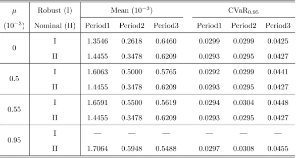
Various nominal portfolio strategies and robust portfolio strategies are computed by setting different values of the required minimal expected/worst-case expected returnµ. Table 2 shows
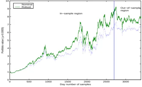
the expected values and the CVaRs at confidence level 0.95 of the corresponding portfolios for each time period. It is obvious that the larger the required minimal expected/worst-case expected return is set, the larger the associated risk would be. From the expected values, we find that the robust optimal portfolio policy always guarantees the required worst-case expected value of µ. However the nominal optimal portfolio policy usually results in a small worst-case expected value although it may have a large expected value (see lines for µ = 0.0005, 0.00055, 0.00095). For the same value of µ, the risk of the robust optimal portfolio policy appears to be larger than the risk of the nominal optimal portfolio policy. It should be mentioned that we only list the CVaRs calculated according to the three sets of samples, and they do not necessarily reveal the real worst-case CVaRs. However, the larger risk is usually rewarded by a higher return, especially a higher worst-case return. Figure 2 illustrates the evolution of the values of the robust optimal portfolio and the nominal optimal portfolio generated by settingµ= 0.0005. It shows that the robust optimal portfolio almost always outperforms the nominal optimal portfolio. For µ = 0.00095, the robust portfolio optimization problem is infeasible. But if µ= 0.00095 is required as the minimal worst-case expected return, the corresponding nominal optimal portfolio, which is obtained by solving (55) withl= 1 and S1 = 2700, becomes infeasible to problem (55) withl= 3 and Si = 900,
i = 1,2,3 since the expected returns of Period2 and Period3 are less than 0.00095. So do the nominal optimal portfolios corresponding to µ = 0.00050 and 0.00055. Moreover, we find that in the sense of worst-case trade-off, the nominal optimal policy generated by setting µ= 0.00095 is dominated by the robust optimal policy generated by settingµ= 0.00055, since we have 0.0005500>0.0005488 for the “worst-case” expected returns and 0.0448<0.0455 for the “worst-case” CVaRs. This together with Figure 2 suggests that the worst-case requirement in the robust portfolio formulation does not affect the average performance of the portfolio substantially.
0 500 1000 1500 2000 2500 3000
0 1 2 3 4 5 6 7 8 9 10
Day number of samples
Portfolio value (
µ
=0.0005)
Nominal Robust
In−sample region
Out−of−sample region
Table 2: Comparison of performances of nominal optimal and robust optimal portfolios.
µ Robust (I) Mean (10−3) CVaR
0.95
(10−3) Nominal (II) Period1 Period2 Period3 Period1 Period2 Period3
0 I 1.3546 0.2618 0.6460 0.0299 0.0299 0.0425
II 1.4455 0.3478 0.6209 0.0293 0.0295 0.0427
0.5 I 1.6063 0.5000 0.5765 0.0292 0.0299 0.0441
II 1.4455 0.3478 0.6209 0.0293 0.0295 0.0427
0.55 I 1.6591 0.5500 0.5619 0.0294 0.0304 0.0448
II 1.4455 0.3478 0.6209 0.0293 0.0295 0.0427
0.95 I — — — — — —
II 1.7064 0.5948 0.5488 0.0297 0.0308 0.0455
Table 3: Expected returns. Asset Expected value
S&P 0.0101110 Gov Bond 0.0043532 Small Cap 0.0137058
3.2.2 Monte Carlo Simulation Analysis
In this part, we perform a Monte Carlo simulation analysis for the robust portfolio optimiza-tion model under the ellipsoidal uncertainty in distribuoptimiza-tions. Notice that a nonempty ellipsoid must contain a smaller box, and at the same time, must be contained by a bigger box. Thus, for both the ellipsoidal and box uncertainties, it is predictable that the simulation results will be similar to each other. As shown in the previous section, the ellipsoidal uncertainty yields a second-order cone program which is more complex than a linear program resulting from the box uncertainty. To reduce the duplicate statements and verify the computational efficiency, we only consider here the case of ellipsoidal uncertainty, i.e, the second-order cone programming model (59).
We take the example given by Rockafellar and Uryasev (2000), where the portfolio is to be constructed by three assets: S&P 500, a portfolio of long-term U.S. government bonds, and a portfolio of small-cap stocks. The expected value and the covariance matrix of returns of these three assets are given in Tables 3 and 4, respectively.
Table 4: Covariance matrix of returns. S&P Gov Bond Small Cap S&P 0.00324652 0.00022983 0.00420395 Gov Bond 0.00022983 0.00049937 0.00019247 Small Cap 0.00420395 0.00019247 0.00764097
In the example, the discrete sample space of random returns consists of 1000 samples, which are generated via the Monte Carlo simulation approach by assuming a joint normal distribution. We set β = 0.95, w0 = 1, x = (0,0,0)T and x = (1,1,1)T. For the sake of
simplicity, the scaling matrix of the ellipsoid A is assume to be a diagonal matrix ρI, where ρ is a nonnegative parameter.
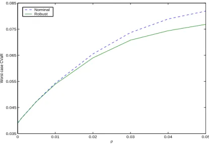
It should be mentioned that the nominal optimal portfolio is obtained by solving model (59) with A = 0, i.e., ρ = 0. The worst-case CVaR of the nominal optimal portfolio is obtained from solving model (59) by setting x = “nominal optimal portfolio”. For both nominal optimal and robust optimal portfolios, we get a set of minimal worst-case CVaRs associated with different values ofρand the fixed value ofµ=−0.03. A part of the numerical results is illustrated in Figure 3, which shows that the worst-case CVaR/risk grows as the value of the uncertain parameter ρ increases. More important observation is that the gap between the two curves becomes larger as ρ increases, which demonstrates the advantage of the robust optimization formulation in the situation where the uncertainty grows.
0 0.01 0.02 0.03 0.04 0.05
0.035 0.045 0.055 0.065 0.075 0.085
ρ
Worst case CVaR
Nominal Robust
Figure 3: Worst-case CVaR of nominal optimal and robust optimal portfolios.
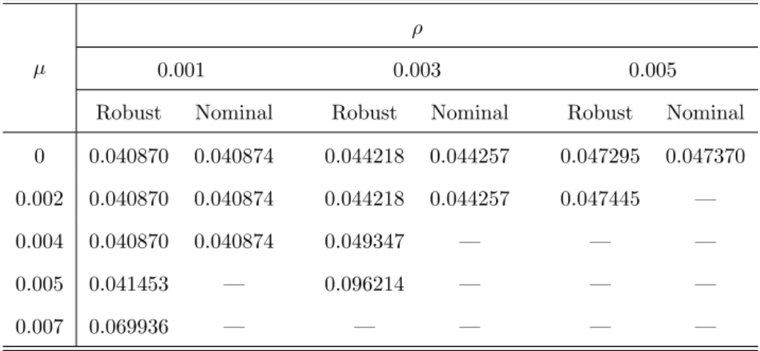
Table 5 shows a part of the comparison results corresponding to several values of µ and ρ, where the phenomenon demonstrated by Figure 3 can also be observed. Table 5 indicates
Table 5: Worst-case CVaR of nominal optimal and robust optimal portfolios according to different values ofµandρ.
µ
ρ
0.001 0.003 0.005
Robust Nominal Robust Nominal Robust Nominal 0 0.040870 0.040874 0.044218 0.044257 0.047295 0.047370 0.002 0.040870 0.040874 0.044218 0.044257 0.047445 —
0.004 0.040870 0.040874 0.049347 — — —
0.005 0.041453 — 0.096214 — — —
0.007 0.069936 — — — — —
that the portfolio problems become infeasible when eitherµorρincreases to a certain degree. For example, the nominal optimal portfolio obtained by solving (59) withρ = 0 is infeasible to (59) with ρ = 0.005, though problem (59) with ρ = 0.005 itself is feasible. Thus, by comparison, the robustness of the robust optimal portfolios is evidenced.
4
Conclusions and Future Directions
This paper focuses on the worst-case CVaR minimization problem for the purpose of dealing with the uncertainty of the probability distributions. Application to robust portfolio opti-mization is also demonstrated. In comparison with the original CVaR, numerical experiments imply that the portfolio selection model using the worst-case CVaR as the risk measure per-forms robustly in practice, and provides more flexibility in portfolio decision analysis.
We can also formulate the robust portfolio optimization problem in the form of maximizing the worst-case expected return with constraint on the worst-case CVaR. For example, in the case of the mixture distribution uncertainty, noting that
WCVaRβ(x) = min
α∈Rmaxi∈L F
i
β(x, α)≤θ
if and only if there exists α such that max
i∈L F
i
β(x, α)≤θ,
we can formulate the corresponding robust portfolio selection problem as the following linear program with variables (x,u, α, µ)∈ Rn× Rm× R × R:
where θ in (20) is a predetermined bound on the worst-case CVaR. The robust portfolio optimization problem of this form can be similarly formulated as a linear program and a second-order cone program for the other two types of uncertainties.
We should emphasis that a reasonable specification of the uncertainty set is the key issue for successful practical application, which is left for further investigation. The specification should be problem oriented. Particular methods should be employed due to the particularity of the problems. Huang et al. (2006) show that it is a natural alternative to formulate the portfolio selection problem with uncertain exit time within the worse-case CVaR framework, where the specification of uncertainty set driven by exogenous and endogenous exiting factors is extensively discussed.
Anyway, we just present in this paper a simple application of worst-case CVaR to port-folio optimization to illustrate our methods. Many other applications of worst-case CVaR in financial optimization and risk management, such as hedging, index tracking, credit risk management and decentralized risk management can also be easily implemented.
Acknowledgments
This work is partly supported by the Informatics Research Center for Development of Knowl-edge Society Infrastructure, Graduate School of Informatics, Kyoto University, Japan. The work of the first author is also supported by the National Science Foundation of China (No. 70401009). The work of the second author is also supported by a Grant-in-Aid for Scientific Research from Japan Society for the Promotion of Science. The authors are grateful to two anonymous referees for their helpful suggestions and comments.
References
[1] Acerbi, C., D. Tasche. 2002. On the coherence of expected shortfall. Journal of Banking and Finance 261487-1503.
[2] Alizadeh, F., D. Goldfarb. 2003. Second-order cone programming. Mathematical Pro-gramming Ser. B 953-51.
[3] Andersson, F., H. Mausser, D. Rosen, S. Uryasev. 2001. Credit risk optimization with conditional value at risk criterion.Mathematical Programming Ser. B 89273-291. [4] Artzner, P., F. Delbaen, J. M. Eber, D. Heath. 1999. Coherence measures of risk.
Math-ematical Finance 9 203-228.
[5] Bazaraa, M. S., H. D. Sherali, C. M. Shetty. 1993.Nonlinear Programming: Theory and Algorithms, Second Edition. John Wiley & Sons, New York.
[6] Ben-Tal, A., A. Nemirovski. 2002. Robust optimization — methodology and applications. Mathematical Programming Ser. B 92453-480.
[7] Ben-Tal, A., T. Margalit, A. Nemirovski. 1999. Robust modeling of multi-stage portfolio problems.High Performance Optimization Techniques, Chapter 12. Eds. J. B. G. Frenk, K. Roos, T. Terlaky, S. Z. Zhang, Kluwer Academic Publishers.
[8] Black, F., R. Litterman. 1992. Global portfolio optimization.Financial Analysts Journal
4828-43.
[9] Bogentoft, E., H. E. Romeijn, S. Uryasev. 2001. Asset/Liability management for pension funds using CVaR constraints.Journal of Risk Finance 3 57-71.
[10] Costa, O. L. V. and A. C. Paiva. 2002. Robust portfolio selection using linear-matrix inequality.Journal of Economic Dynamics & Control 26889-909.
[11] El Ghaoui, L., M. Oks, F. Oustry. 2003. Worst-case Value-at-Risk and robust portfolio optimization: A conic programming approach.Operations Research 51543-556.
[12] Fan, K. 1953. Minimax theorems.Proceedings of National Academy of Science 3942-47. [13] Goldfarb, D., G. Iyengar. 2003. Robust portfolio selection problems. Mathematics of
Operations Research 28 1-38.
[14] Hall, J. A., B. W. Brorsen, S. H. Irwin. 1989. The distribution of futures prices: A test of the stable Paretian and mixture of normals hypotheses.Journal of Financial and Quantitative Analysis 24105-116.
[15] Halld´orsson, B. V., R. H. T¨ut¨unc¨u. 2003. An interior-point method for a class of saddle-point problems.Journal of Optimization Theory and Applications 116 559-590.
[16] Høyland, K., S. W. Wallace. 2001. Generating scenario trees for multistage decision problems.Management Science 47295-307.
[17] Huang, D. S., S. S. Zhu, F. J. Fabozzi, M. Fukushima. 2006. Robust CVaR approach to portfolio selection with uncertain exit time. Technical Report 2006-1, Department of Applied Mathematics and Physics, Graduate School of Informatics, Kyoto University, http://www.amp.i.kyoto-u.ac.jp/tecrep.
[18] Ji, X. D., S. S. Zhu, S. Y. Wang, S. Z. Zhang. 2005. A stochastic linear goal programming approach to multi-stage portfolio management based on scenario generation via linear programming.IIE Transactions 37957-969.
[19] Konno, H., H. Waki, A. Yuuki. 2002. Portfolio optimization under lower partial risk measures.Asia-Pacific Financial Markets 9 127-140.
[20] Lobo, M. S., S. Boyd. 2000. The worst-case risk of a portfolio. Technical Report, http://faculty.fuqua.duke.edu/∼mlobo/bio/researchfiles/rsk-bnd.pdf.
[21] Lobo, M. S., L. Vandenberghe, S. Boyd, H. Lebret. 1998. Applications of second-order cone programming.Linear Algebra and Its Applications 284 193-228.
[22] Markowitz, H. M. 1952. Portfolio selection. Journal of Finance 777-91.
[23] Martellini, L., B. Uroˇsevi´o. 2005. Static mean-variance analysis with uncertain time hori-zon, forthcoming inManagement Science.
[24] Mulvey, J., G. Erkan. 2003. Decentralized risk management for global P/C insurance companies. Working paper, Department of Operations Research and Financial Engineer-ing, Princeton University.
[25] Ogryczak, W., A. Ruszczy´nski. 2002. Dual stochastic dominance and related mean-risk models.SIAM Journal on Optimization 1360-78.
[26] Peel D., G. J. McLachlan. 2000. Robust mixture modelling using the t distribution. Statistics and Computing 10339-348.
[27] Pflug, G. 2000. Some remarks on the Value-at-Risk and conditional Value-at-Risk. Proba-bilistic Constrained Optimization: Methodology and Applications. Ed. S. Uryasev, Kluwer Academic Publishers, Dordrecht.
[28] Philippe, J. 1996.Value at Risk: The New Benchmark for Controlling Market Risk. Irwin Professional Publishing, Chicago.
[29] RiskMetricsTM. 1996. Technical Document, 4-th Edition. J. P. Morgan.
[30] Rockafellar, R.T., S. Uryasev. 2000. Optimization of conditional Value-at-Risk. Journal of Risk 2 21-41.
[31] Rockafellar, R. T., S. Uryasev. 2002. Conditional Value-at-Risk for general loss distribu-tions.Journal of Banking and Finance 261443-1471.
[32] Sturm, J. 2001. Using SeDuMi, a matlab toolbox for optimization over symmetric cones. Department of Ecnometrics, Tilburg University, The Netherlands.
[33] Topaloglou, N., H. Vladimirou, S. A. Zenios. 2002. CVaR models with selective hedging for international asset allocation.Journal of Banking and Finance 261535-1561.