Utility Programs Reference Manual 1 op_vuanim Utility

1

op_vuanim Utility

Animations of simulations provide useful support for analyzing, verifying, and troubleshooting dynamic models. Simulations developed within OPNET’s modeling editors offer animations for investigating the behavior and

performance of dynamic models. This chapter describes the overall architecture of OPNET’s model animation system, as well as the usage of the op_vuanim program, which provides a means of viewing animations both during

simulation, and afterwards.

Animation System Architecture

The model animation system architecture is the basis for animation services within OPNET products. It addresses the basic r

ange of

• definitions of fundamental animation concepts such as animation flow, animation request, and viewer

• animation data routing options, which include direct viewing and animation history files

• animation activation mechanisms, which include simulation environment attributes and animation probes

• conversion of animations between the history file and script file forms • detailed presentation of the syntax and function of animation script files In defining the animation architecture, it is necessary to reference standard, contingent components and systems within OPNET products, such as:

• simulation: one output product of OPNET modeling environments is a

simulation, a stand-alone program that performs event-driven modeling of a system. Simulations can generate animations as a form of documenting the dynamic characteristics of the modeled system.

• Simulation Kernel: simulations are built from OPNET-supplied and

user-defined components; the core OPNET simulation algorithms and services are contained in a object code library known as the Simulation Kernel, which is linked into simulations as they are built. Animation generation is one of many services supported by the Simulation Kernel.

• Kernel Procedure: the programming interface of the Simulation Kernel is defined by a set of Kernel Procedures (often abbreviated as KPs) which each perform a particular operation for processes and procedures within a simulation. KPs are organized into packages that address particular

simulation services. Animation services are provided by the Anim package of KPs within the Simulation Kernel.

• simulation debugger: the Simulation Kernel incorporates a command-driven

debugging interface for analyzing and controlling simulation behavior, known as the simulation debugger. The simulation debugger supports single-event control of simulation execution, and provides many diagnostic information features.

• probe: by default, simulations do not typically generate files of output data;

instead, specific results of interest to the user are specified by probes set on particular simulation objects. Probes are contained within a file known as a probe list, which is applied to simulations to activate data collection.

Animation probes support the activation of animation data generation within a simulation.

Animation Fundamentals

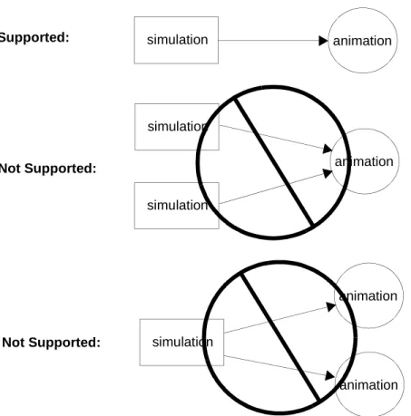
OPNET animations can be produced and recorded during simulations. Animations and simulation runs have a one-to-one correspondence. Multiple simulation runs cannot contribute to a single animation. A simulation cannot produce more than one animation.

When a simulation run is initiated, the user specifies whether animation data will be recorded and how it will be routed. If “record animation” is specified, all animation data generated by a simulation run will be routed as indicated, contributing to a single animation. A simulation cannot change the routing of animation data while executing.

Figure 1-1 Simulation/Animation Relationships

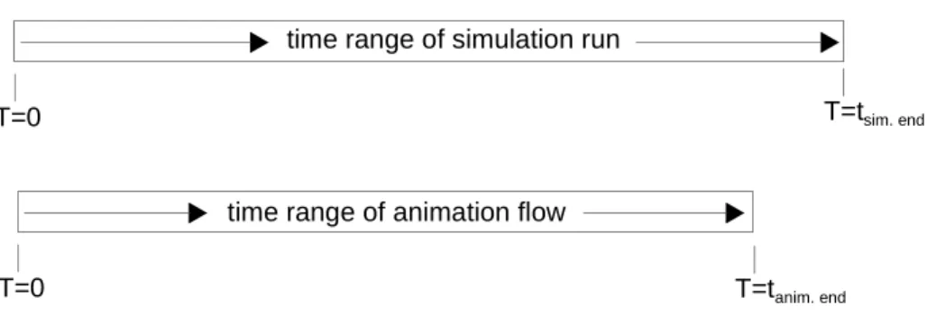
Animations depict dynamic simulation conditions. As simulation events occur at various points in simulation time, they generate animation data that is tagged with the associated simulation time. Thus, all animation data are associated with simulation time values. An animation time range always falls within the time range of the associated simulation run. Simulation runs have a beginning and an end in simulation time; likewise, their associated animations have beginnings and ends in simulation time. The first animation data generated by a simulation may begin later than T=0, and the last animation data generated by a simulation may occur well before the end of the run. However, animation data can never occur at negative times, or at times later than the end of the associated simulation run.

As a simulation producing an animation progresses, it typically generates animation data at a large number of irregularly spaced points in simulation, which are spread in small bursts throughout the simulation. Animation data depicting a simulation event is usually produced as soon after the event as possible, so that (synchronized viewing of animation data is possible (i.e.,

simulation animation

Supported:

Not Supported:

Not Supported:

simulation

simulation

animation

animation

animation simulation

before the simulation progresses to another event. The previous statements are usually true, but since users can generate custom animations through flexible Kernel Procedure invocations, it is possible to cluster the output of animation data into only a few large bursts that occur at the beginning, end, or some intermediate point in a simulation.)

Because animations are described by bursts of data that occur over a range of time, these bursts form a flow of data. The term animation flow refers to the sequence of animation data generated by a simulation run. As will be explained later in this chapter, animation flows can be stored in a file, conveyed to another process using network protocols, or processed and displayed by a viewing program.

Figure 1-2 Comparison of Typical Simulation and Animation Flow Time Ranges

Bursts usually consist of animation data generated at the same simulation time. The fine-grain structure of bursts is a series of animation requests. Animation requests are the smallest units of animation data. Each animation request is associated with a single simulation time, a single simulation event, and a single source within the simulation (e.g., a specific process). Typically, animation flows will contain thousands of animation requests.

There are over forty types of animation requests supported by the OPNET system. New types of requests cannot be defined by users.

Simple animation requests describe a single graphical operation, such as drawing a line, and contain all the data required for the operation. A more complex animation request may describe a compound graphical operation, such as moving a symbol along a path. Such a request will depend on data contained in other requests--however, no matter how complex an animation request is, it never describes graphical operations associated with different simulation times or events.

time range of simulation run

T=0 T=tsim. end

time range of animation flow

Thus it is possible to segment an animation flow according to simulation times or events; such divisions always occur on request boundaries since these properties never change within a single animation request.

Figure 1-3 Animation Flows are Composed of Animation Requests

Animation flows can describe graphical operations performed within one or more abstract display regions called viewers. A viewer is a rectangular region with an internal coordinate system. Most animation requests are targeted to a particular viewer, as identified by a viewer ID contained within the request. Some administrative requests deal with animation-wide issues, and do not generate visible output in a particular viewer; these requests do not contain viewer IDs. Viewers can be opened or closed by specific request types at any stage of an animation flow. However, viewers must be opened before requests can be targeted to them. Once a viewer has been closed, it cannot accept any further requests.

Animation requests specify graphical operations in terms of viewer coordinates. Each viewer has its own coordinate system, but the viewer coordinate systems share the following common properties:

• two-dimensional (X is the horizontal axis, Y is the vertical axis) • origin is the upper-left corner

• positive X direction points right, positive Y direction points down

• only integral, non-negative coordinates are supported; the upper limit on coordinate values is 32,766

• coordinates are measured in units of pixels

• coordinate system extends beyond visible region of viewer

T=0 T=tanim. end

R

animation flow:

R R R R R R

R R R R R R

R R R R

R R R R R

R R R R

R R R

(T=10,Ev=210)

(T=10,Ev=212)

(T=14,Ev=216)

(T=14,Ev=220) association of requests with simulation events and times:

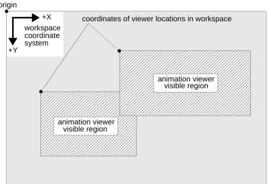
The request that opens a viewer specifies its location within the workspace coordinate system, and its initial size. Viewers may have intersections within the workspace, in which case the viewers that are opened later will initially overlap the viewers opened earlier. The size of a viewer determines the rectangular region of the viewer’s coordinate system that is visible, but it does not limit graphical operations from being performed outside of this visible region. The visible region of a viewer can be changed by scrolling the viewer via a specific request type. Due to the limitations of the viewer coordinate system, the visible region cannot be scrolled into the (X,Y) plane quadrants with negative

coordinate values.

Figure 1-4 Animation Viewers within Workspace Coordinate System

+Y

+X workspace coordinate system

animation viewer coordinates of viewer locations in workspace

visible region

animation viewer visible region origin

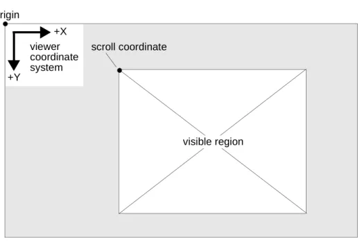
Figure 1-5 Animation Viewer Coordinate System

The abstract concept of a viewer is realized within the animation viewing program op_vuanim, which creates editor windows for each viewer. Viewer windows can be manipulated using the standard GUI operations for moving, resizing, scrolling, and circulating windows. These operations do not affect the animation being viewed, but change the presentation of the animation. Details of op_vuanim features appear later in this chapter.

Flow Activation and Routing

Animation flows are not generated as a default by-product of simulations. Instead, animation flows must be specifically activated by the user. Flow activation is accomplished through a combination of simulation environment attributes and animation probes within a probe list applied to the simulation. Besides activating a flow, the animation-related environment attributes of a simulation specify how the flow will be routed (several options are available for routing the generated animation data). In addition to specifying which types of animation will be produced by which model objects, animation probes specify viewer options and animation time-range limits. Both types of activation requirements, animation-related environment attributes and animation probes, are discussed in this section.

There are two routing options for animation flows generated by a simulation: (1) routing to direct viewing in op_vuanim; (2) routing to an animation history file. If neither of these routing options is selected by the appropriate simulation environment attributes, no animation flow will be generated. Each of these routing options are discussed in separate subsections below.

+Y

+X viewer coordinate system origin

scroll coordinate

Direct Viewing

In the direct viewing option, animation flow data is routed directly from an executing simulation to a concurrently executing instance of the op_vuanim program. The method of communication between the simulation and

op_vuanim is a low-level network datagram protocol. The use of the network protocol supports both local and remote viewing scenarios: in a remote viewing scenario, op_vuanim executes on a different host computer than the simulation; in a local scenario, op_vuanim executes on the same host computer as the simulation.

The simulation and op_vuanim processes are synchronized by the animation flow, so that the simulation halts progress after it sends an animation request to op_vuanim, until it receives an acknowledgment that op_vuanim actually displayed the request. With this synchronization, a user can view simulation progress at an adjustable pace, without having the simulation continue far ahead of the user’s position in the animation flow, thus generating a large backlog of animation flow data. The synchronization of the direct viewing option is also critical when the option is used in conjunction with the simulation debugger, because it guarantees that a command specified in the debugger can be immediately reflected in the animation flow displayed in op_vuanim. This immediate feedback stems from the fact that the simulation is restricted from getting ahead of either the simulation debugger command loop or the animation flow playback of op_vuanim.

Figure 1-6 Flow Routing Option: Direct Viewing

simulation op_vuanim

process process

animation flow common host computer

local viewing scenario:

remote viewing scenario:

simulation op_vuanim

process animation flow process

sim. host computer viewing host computer

The direct viewing option is specified by the anim_view environment attribute of simulations. Setting this Boolean attribute to TRUE as shown below causes a simulation to attempt to communicate with an op_vuanim process. Additional information in the form of environment attribute assignments may need to be provided to specify communication parameters.

Figure 1-7 Specifying Direct Viewing via the anim_view Flag

The network datagram protocol used as the communication channel between an executing simulation and a op_vuanim process is UDP (User Datagram Protocol), which relies on the datagram delivery services of the

industry-standard IP networking protocol (both of these protocols are part of the DoD-developed TCP/IP protocol suite). Each animation request is

encapsulated in a UDP packet, and forwarded to the op_vuanim process. Two types of acknowledgment packets are returned from the op_vuanim process to its associated simulation for each request: an acknowledgment that the request was received, and an acknowledgment that the request was displayed.

Time-out features are built into the Simulation Kernel so that it will retransmit animation requests that have not been acknowledged within an adequate time interval.

Figure 1-8 Animation Flow Communication Over UDP/IP % op_runsim -net_name angen -anim_view <...>

encapsulated request packets flow

simulation op_vuanim

process process

R

_R

A

IP IP UDP

A

encapsulated acknowledgment packets flow to the simulation process

to the op_vuanim process

Note: the packets in this diagram are only intended to depict data types and flow directions; except in special conditions, there is no more than a single packet in transit between the simulation and op_vuanim processes at a time.

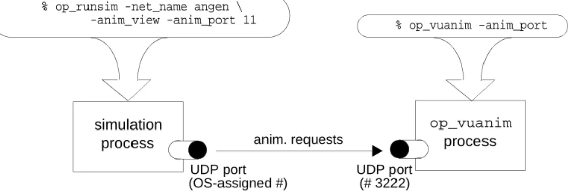
In order for UDP datagrams to travel between the simulation and op_vuanim processes, these processes must be aware of each other’s IP network address and UDP port number. Since the interprocess communication is still based on UDP/IP, these data items are required when the simulation and op_vuanim processes are executing on the same host computer. A port number identifies a port opened by a process for a protocol using the delivery services of IP, and distinguishes the process as a unique destination for the contents of IP packets. Address and port number data is obtained using a client/server strategy that is typical for IP-based services.

The op_vuanim process is considered a server process: it offers the animation viewing service to client simulations on the network. For this strategy to work, the op_vuanim process must begin execution before simulations attempt to connect with it. During initialization, op_vuanim establishes a UDP port on its host computer. The default port number is a fixed value that is also the default expectation of client simulations.

A client simulation derives the IP address of the op_vuanim host computer from the anim_host environment attribute. This attribute provides the simulation with the network name of the op_vuanim host computer; the host’s name is

translated into the host’s IP address using a name server available on the network, or the simulation host computer’s /etc/hosts file. The default value of the anim_host environment attribute is “localhost”, which usually translates to the loopback address of the simulation host computer. Thus the anim_host environment attribute typically does not need to be specified in the local viewing scenario.

Figure 1-9 Specifying the op_vuanim Host via the anim_host Flag

Once an op_vuanim process receives an initial communication establishment packet from a simulation, it can extract the simulation’s host computer IP address from the packet, for use in future acknowledgment packets. The op_vuanim program thus does not require user specification of the IP address of the simulation’s host computer.

As mentioned previously, the default UDP port number of op_vuanim is known to simulations. This port number is hardwired to 3211, which should not interfere with any widely-used, IP-based service. However, particular installations may need to reserve this port number for internally developed or commercial software systems. In such cases, both op_vuanim and simulations can be informed that another UDP port number must be used. An alternative port number is not specified directly, but is specified as an offset from the default port number of 3211. This relative port offset is known as the animation port, and is specified to both op_vuanim and simulations via the anim_port environment % op_runsim -net_name angen -anim_view -anim_host guardian

attribute. The default value of anim_port is 0, so that the default UDP port number is 3211 + 0 = 3211; setting anim_port to 5 will result in a UDP port number of 3211 + 5 = 3216. Provided that an op_vuanim process and a simulation process agree on the value of anim_port, they can establish communications.

A simulation is assigned a free UDP port number by the operating system when it opens up a port to communicate with op_vuanim. The simulation’s port number varies from execution to execution, and is not of interest to the user since it is directly conveyed to op_vuanim in the communication establishment packet.

Figure 1-10 Matching Simulation and op_vuanim Animation Ports

Another problem related to animation ports arises when more than one

op_vuanim process is executing on a single host computer. It is impossible for two ports on the same host to share a port number, so multiple op_vuanim processes must have different animation port value. op_vuanim tries to open a UDP port based on the specified animation port, but if it detects that the request port number is in use by another process, it increments the animation port by one and tries to open a UDP port based on the new value. This "bump up" procedure continues indefinitely until a free port is found. Thus multiple op_vuanim processes can be spawned on a single host computer without specifying different animation port values, since each process will find an available port.

In order for a simulation to communicate with one of multiple op_vuanim processes on a single host computer, the animation port number should be determined by reading it from the middle-right status strip within the

environment of the desired op_vuanim instance. Once determined, the particular animation port can be targeted by executing a simulation with the same value assigned to the anim_port environment attribute.

The UDP and IP protocols do not guarantee delivery of datagrams, and do not provide retransmission of datagrams lost in transit due to LAN collisions, routing problems, or other network lapses. Thus the communicating simulation and op_vuanim processes must detect packet losses and perform retransmissions

simulation op_vuanim

process process

% op_vuanim -anim_port

UDP port (# 3222) anim. requests

UDP port (OS-assigned #)

% op_runsim -net_name angen \ -anim_view -anim_port 11

parameterized to meet the network delay conditions experienced at different installations. The two retransmission parameters affect: (a) the amount of time that a simulation will wait for a request reception acknowledgment from an op_vuanim process before retransmitting; (b) the number of times a simulation will retransmit a request before giving up. These parameters are respectively set by the anim_timeout and anim_attempts environment attributes. The anim_timeout attribute accepts a floating-point value in units of seconds; its default value is 3.0 seconds. The anim_attempts environment attribute accepts an integer value; its default value is 5 retries. The default values of these attributes have been determined to provide a viable connection in a fairly loaded LAN environment.

Figure 1-11 Specifying Retransmission Parameters via the anim_timeout and anim_attempts Flags

In many user installations, the parameters that affect direct viewing of animation flows will stay constant over relatively long periods of time. Thus the

corresponding environment attributes can be assigned stable values in the Environment Database, as shown on the next page. Notice that the anim_view environment attribute is not typically assigned in the Environment Database, since the decision to select the direct viewing option is best left open until a simulation is executed.

Figure 1-12 Setting Animation Communication Parameters in the Environment Database

This first packet received by op_vuanim from a simulation indicates that an animation flow will follow. As a result, op_vuanim enters an active mode for the playback of the animation flow. Acceptance of the animation flow is indicated by a message in the message area and header strip text that indicates the name of simulation. The initial mode of the animation flow is paused; the flow will not

% op_runsim -net_name angen -anim_view -anim_host guardian \

-anim_timeout 2.5 -anim_attempts 8

<...>

# animation communication parameters anim_host: guardian

anim_port: 6 anim_attempts: 8 anim_timeout: 2.5 <...>

begin playback until a playback operation is activated from op_vuanim’s button panel. The buttons associated with operations that can initiate the playback are displayed on the next page; more information on these operations is presented later in this chapter.

Figure 1-13 Animation Flow Acceptance Messages

Figure 1-14 op_vuanim Animation Playback Operation Button op_vuanim message area

op_vuanim header strip

flow type indication and simulation name

and host computer

op_vuanim 8.0.A (c) 2001 OPNET Technologies, Inc. Paused Simulation: rtesamp.sim

simulation name

play anim. flow

step to next anim. request

step to next sim. event

step to next sim. time

Until an accepted animation flow is terminated by the simulation or by an op_vuanim user action, op_vuanim will not accept an animation flow from another simulation. Should another simulation attempt to establish

communications, op_vuanim will issue an error message, and the rejected simulation will issue an error message while continuing to execute without sending further animation packets to op_vuanim. Likewise, when playing back an animation history file, op_vuanim will reject an incoming animation flow. Figure 1-15 Animation Flow Rejection Messages

Most animation flows are not self-contained; i.e., they depend on the existence of other referenced resources to be properly displayed without error. Examples of other referenced resources are models used as the diagram context for animations, maps used as model backdrops, trajectory or orbit files used as movement paths, and user-defined icons. These resources are referenced in the animation flow data, rather then being fully integrated, in order to avoid redundant storage of the resources and any associated version-consistency problems. However, the referencing of resources introduces the problem of access to these resources. Provided that op_vuanim is executing in a user context (as defined by the Environment Database and the model directories referenced therein) that includes the needed resources, an animation flow with resource references can be properly played back by op_vuanim. In situations where an animation flow is being displayed by a op_vuanim process in a different user context or host computer than the source simulation, the referenced resource files must be copied to the op_vuanim process

environment so that it can properly access and utilize them in the animation playback.

op_vuanim message area

simulation name and host computer

History Files

In the animation history file option, animation flow data is routed from an executing simulation into a binary data file that grows in size as the simulation progresses. When a simulation producing an animation history file is completed, the history file can be loaded and viewed in op_vuanim. History files provide the following benefits:

• long-term storage of an animation in a format that can be immediately viewed with no additional preparation

• elimination of animation latency caused by simulation computation and inter-process communication and synchronization

• repeated viewing of an animation without recomputation • convenient format for transmission of animations to colleagues

Animation history files are the favored option for animation routing, due to the time savings they afford. In most cases, the direct-viewing alternative is used primarily with the simulation debugger because animation history files cannot be viewed during a simulation run and therefore cannot serve as a feedback mechanism for a debugging session.

Figure 1-16 Flow Routing Option: History File

op_vuanim process during simulation:

after simulation:

animation history file

animation flow simulation

process _animation

history file animation flow

growth during simulation

The history file option is specified by the anim_hist environment attribute of simulations. This string attribute accepts the base name of the animation history file, without the file’s path or type suffix. The file type suffix .ah (an acronym of “animation history”) is appended to the base name. Note that new animation history files are stored in the primary model directory, and are not coupled to the location of the simulation that generated them.

Figure 1-17 Specifying a History File via the anim_hist Flag

After an animation history file is created, and the simulation that generated it has finished executing, the history file can be read into op_vuanim via the Read Animation History operation.

Once a selection from the menu has been made, the header strip text indicates the name of the loaded history file. Unlike typical read operations that deal with models, the Read Animation History operation does not transfer the full contents of the animation history file to virtual memory before displaying it. Instead, a portion of the animation history file is read into a virtual memory buffer that stores the requests until needed in the animation playback. When the buffer has been depleted of requests by the playback procedure, it is again filled from the history file, until the whole history file has been processed through the buffer. The size of the history buffer is fixed at 8 KB, and cannot be modified.

Figure 1-18 Read Animation History Operation Button

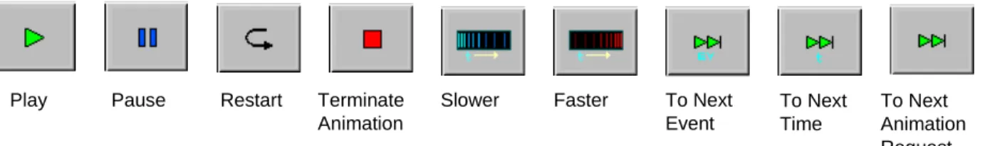
After the initial buffer of an animation history file has been loaded by the Read Animation History operation, the animation flow is active but paused. The flow will not begin playback until a playback operation is activated from op_vuanim’s button panel. Operations that active playback, pause, return to start, etc., are displayed on the next page. Note that these are the same operations that can initiate the playback of a direct view animation, with the addition of the Restart Animation Flow operation, which restarts the currently loaded animation from its % op_runsim -net_name angen -anim_hist ang2

op_vuanim header strip

flow type indication and history name

Animation History Header Strip Example

Figure 1-19 op_vuanim Animation Playback Operation Buttons

The caveat appearing in the last section regarding referenced resources also applies to animation flows derived from history files. Since animation history files may contain references to supporting files such as models, maps, trajectory or orbit files, or icons, the referenced resources must be accessible to

op_vuanim to guarantee an error-free animation playback. Dual Routing

The direct viewing and history file routing options of animations can be

combined within a single simulation, so that a simulation’s animation is viewable as the simulation executes, but is also available for repeated viewing later. Dual routing of a simulation’s animation flow is selected by specifying both the anim_view and anim_hist environment attributes, as shown in Figure 1-20. Under dual routing, the direct viewing option is still independent of the history file option, so if a user exits op_vuanim and thus shuts down direct viewing of an animation flow, the simulation will continue to produce an animation history file.

Figure 1-20 Specifying Dual Routing of an Animation Flow

Script Files

Although there are only two direct routing options for animation flows generated by a simulation (direct viewing in op_vuanim, or writing to a history file), a detour can be inserted into the animation history file routing option for the purpose of editing or enhancing an animation flow. Animation history files contain binary data that is encoded in a OPNET proprietary format, and so cannot be directly manipulated by users. However, animation history files can be converted into animation script files, which are equivalent descriptions of the captured

animation flow, encoded in an ASCII scripting language that can be viewed and modified within a standard text editor. Script files can also be converted back into history files, thus providing the ability to edit or add to an animation history file indirectly through the script form.

dddd

dddd

Play Pause Restart Terminate Slower

Animation

Faster To Next

Event

To Next Time

To Next Animation Request

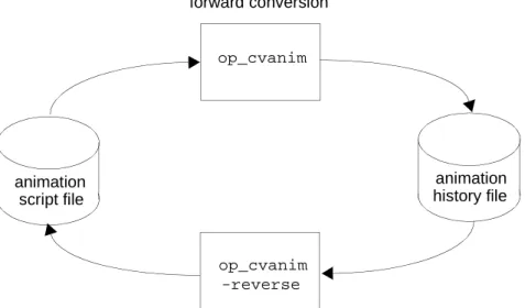
Conversion of an animation flow between the history file and script file forms is performed by the op_cvanim utility program. op_cvanim determines the direction of conversion by the Boolean value of the environment attribute “reverse”: forward conversion (“reverse” set to FALSE) produces a history file from a script file, and reverse conversion (“reverse” set to TRUE) produces a script file from a history file, as illustrated in the following diagram.

Figure 1-21 Animation History / Script Conversion

The diagram below puts the conversion cycle into the larger context of animation history routing.

Figure 1-22 Animation History Editing Data Flow Diagram op_cvanim

animation history file animation

script file

op_cvanim forward conversion

reverse conversion -reverse

op_cvanim

animation history file animation

script file

op_cvanim -reverse

simulation

op_vuanim process

process Text editor

op_cvanim obtains the base name of the animation from the string environment attribute “m” (the animation base name should not include a file path or file type suffix). The file type suffix .as is appended to the base name to form the animation script file name, and the suffix .ah is appended for the animation history file name. Animation history or script files created by op_cvanim are stored in the working model directory, and are not coupled to the file from which they were converted.

Once in script form, an animation flow is available for symbolic viewing and editing. Each request of an animation flow is described by a single statement in a script (the scripting language is presented in a later section of this chapter). Script editing may include adding new requests, deleting undesirable requests, or modifying the arguments of requests. Animation scripts may also be

completely entered manually, for the purpose of prototyping an animation concept. If statements in an animation script have syntax errors, op_cvanim will detect these in the process of converting the script file to a history file, and will issue an error and cancel the conversion.

Animation Probes

An animation routing option can be selected via the simulation environment attributes anim_view or anim_hist, causing the simulation to activate an animation flow. In the direct viewing option, an activated animation flow will establish communications with the indicated op_vuanim process, and a file will be created in the animation history option. However, an activated animation flow will not contain any animation requests if no animation probes have been applied to the simulation through the probe environment attribute. Animation probes are required to identify the objects enabled for animation request generation. If no probes are specified in a probe list, or if no value is assigned to the probe environment attribute, then no objects are enabled to generate animation requests.

There are three types of animation probes.

• An automatic animation probe enables an animation algorithm built into the Simulation Kernel called a representation; this algorithm generates a complete animated depiction of a simulation model in a single viewer, including a model diagram and dynamic elements that move or change in the diagram.

• A custom animation probe enables a simulation object and all of its

sub-objects to issue custom animation requests. Custom animation requests are specified by Anim package KPs invoked by user-defined processes or procedures within a simulation, but requests will not be issued into the simulation’s animation flow unless the object containing the process or procedure making Anim invocations is enabled by a custom animation probe. • A statistic animation probe animates output vector results that are generated

A probe list can include any number of automatic and custom animation probes, in addition to non-animation probes. The animation requests enabled by animation probes are combined into the single simulation animation flow, interleaved in the order of generation. Animation probes are generally independent and do not affect each other; the only exception to this occurs when a custom animation probe references the same object as another custom animation probe, or an object hierarchically affected by another custom animation probe. For a description of this type of interaction, refer to Custom Probes on page UP-1-24.

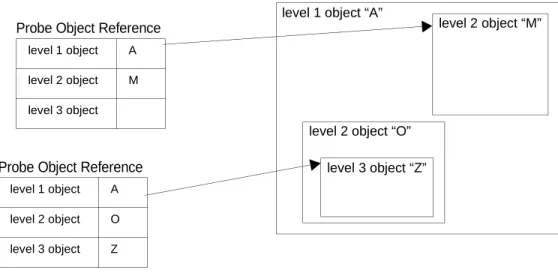
Automatic, custom, and statistic animation probes share a large number of common attributes that specify data required by all probes, and data required to describe the probes’ time range and viewer options. The general probe

attributes include the name attribute that identifies the probe object within the probe list, and several attributes used to hierarchically identify the object targeted by the probe. These attributes are not discussed in detail in this chapter, but the diagram below illustrates the targeting of a simulation object by an animation probe (note that objects are described in an abstract sense). Figure 1-23 Simulation Object Targeting by Animation Probes

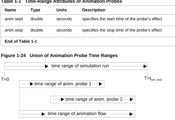
Two probe attributes define the time range over which an animation probe will enable animation requests issued from its targeted objects. These attributes are described in the table below. By default, the anim start attribute has a value of 0, and the anim stop has an infinite value; unless these attributes are explicitly assigned different values, an animation probe will be in effect during the full duration of a simulation. Setting the anim start attribute to a positive, non-zero value, or setting the anim stop attribute to a value less than the duration of the associated simulation will result in a reduced time range for the probe.

Restricted probe time ranges are useful in limiting an animation to only level 1 object “A”

level 2 object “M”

level 2 object “O” level 3 object “Z” level 1 object A

level 2 object O level 3 object Z Probe Object Reference

level 1 object A level 2 object M level 3 object

interesting events that fall within a specific segment of time. Since each animation probe has its own time range attributes, the aggregate time range of an animation flow actually spans the earliest probe start time and the latest probe stop time.

Figure 1-24 Union of Animation Probe Time Ranges

Animation probe time ranges are not entirely strict; a few types of animation request can "cut through" the limits of a time range, adding themselves to a simulation’s animation flow even though the request times fall outside of the nominal time range of the associated animation probe. The request types that cut through probe time ranges have the following common properties: (a) they don’t directly perform a graphical operation in a viewer; (b) they create an animation resource that is needed by later animation requests. If these types of requests were blocked when issued outside of their associated time range, the associated resources would not exist and later animation requests would cause errors upon referring to the missing resources. Activities that can cut through time ranges include the creation of viewers, and the creation and definition of macros (introduced later in this chapter).

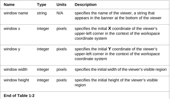
Viewers are an important part of the animation playback environment. Viewers define a display region for a series of related animation requests. All animation probes specify the parameters of an associated viewer using a group of five attributes that are listed in Table 1-2 on page UP-1-22; however, automatic and custom animation probes create viewers under different conditions. Every automatic animation probe creates a viewer with the specified name and initial size, and directs all the animation requests it enables to its viewer. A custom animation probe only creates a viewer based on the probe’s specified

Table 1-1 Time-Range Attributes of Animation Probes Name Type Units Description

anim start double seconds specifies the start time of the probe’s effect anim stop double seconds specifies the stop time of the probe’s effect End of Table 1-1

time range of simulation run

T=0 T=tsim. end

time range of animation flow time range of anim. probe 1

parameters if objects it enables issue animation requests that reference the probe’s viewer; other animation requests enabled via custom animation probes may create their own viewers in accordance with the design of the custom animation. Therefore the viewer specified by a custom animation probe may be ignored by some or all of the custom animation requests that it enables.

Four of the five animation probe viewer attributes specify the initial size and location of the viewer’s visible region in workspace coordinates. All of these values can be changed during animation playback within op_vuanim, via a user operation. The initial scroll position of a probe’s viewer cannot be specified in the probe object; it is fixed at the origin of the viewer’s coordinate system. A viewer’s scroll coordinate can be changed through an Anim Kernel Procedure, or by user operations in op_vuanim.

Figure 1-25 Animation Probe Viewer Name Configuration Table 1-2 Viewer Attributes of Animation Probes

Name Type Units Description

window name string N/A specifies the name of the viewer, a string that appears in the banner at the bottom of the viewer window x integer pixels specifies the initial X coordinate of the viewer’s

upper-left corner in the context of the workspace coordinate system

window y integer pixels specifies the initial Y coordinate of the viewer’s upper-left corner in the context of the workspace coordinate system

window width integer pixels specifies the initial width of the viewer’s visible region window height integer pixels specifies the initial height of the viewer’s visible

region End of Table 1-2

Figure 1-26 Animation Probe Viewer Size and Location Configuration

Automatic Probes

An automatic animation probe is set for a single simulation object, and enables requests that create a single animation viewer and perform graphical operations within it. In order to "animate" the probed object, the Simulation Kernel

generates animation requests that display the model diagram that defines the internal structure of the object, in addition to superimposed dynamic elements. For a given model type, the Simulation Kernel may support several different animation algorithms, known as representations. An animation flow can include multiple automatic animation representations, but each must be separately enabled by its own automatic animation probe. A single object can even be probed for different simultaneous representations.

In addition to the general animation probe attributes, automatic animation probes must specify the respective representations they generate. The representation enabled by an automatic animation probe is specified by the representation attribute, displayed in the following table. The possible values of this attribute depend on the type of object being probed.

+Y

+X workspace coordinate system

probe viewer (window x, window y)

visible region window

height

window width

Table 1-3 Special Automatic Animation Probe Attributes

Name Type Description

representation string specifies the name of the automatic animation representation that the probe enables

Custom Probes

A custom animation probe is set for a single simulation object, but it affects all the objects contained within the directly probed object. Custom animation probes enable the set of probed objects to issue custom animation requests. The direct sources of custom animation requests are invocations of the Anim package KPs by processes or procedures associated with simulation objects. If an object contains an animation request-generating process, the requests will only be added to the simulation’s animation flow if a custom animation probe enables requests from the object.

Multiple custom animation probes may be defined in a probe list, and they may be defined in hybrid probe lists that also include automatic animation probes. A custom animation probe is independent of all other custom animation probes if it references an object that is not hierarchically related to any other probed object. On the other hand, a custom animation probe may overlap another custom animation probe by probing an object that is hierarchically related to the other probe’s object. Custom animation probes with overlapping regions of influence produce the following effects: (a) the general request-enabling effect of custom animation probes is simply applied to a region of influence that is the union of the probes’ independent regions of influence; (b) if a process or procedure associated with an object within the intersection of the probe regions of influence issues an Anim package KP with the viewer ID argument set to the symbolic constant OPC_ANIM_ANVID_PBSPEC, then only one of the

probe-specified viewers will display the KP’s result (the affected viewer depends on the order of the probes in the probe list).

In addition to the general animation probe attributes, custom animation probes include an optional probe attribute (label) that can be used to restrict the influence of the probes to Anim package KP invocations that rely on the existence of a particular probe label. If a value is assigned to the “label” attribute, the custom animation probe is considered a labeled probe (a custom animation probe with no value assigned to “label” is considered an unlabeled probe). Labeled probes sacrifice the ability of unlabeled probes to enable animation requests generally throughout their region of influence. Instead, a labeled probe only enables requests from Anim package KP invocations that reference the probe’s associated viewer ID. A labeled probe’s viewer ID can be obtained by invoking the KP op_anim_lprobe_anvid() and passing the probe’s label. Labeled probes provide a useful mechanism for defining custom animation features within a simulation that can be independently enabled or disabled. Table 1-4 Special Custom Animation Probe Attributes

Name Type Description

label string specifies the probe is labeled, and provides the

label text End of Table 1-4

Statistic Probes

Statistic animation probes produce dynamic graphs of simulation results. To get this result, you:

• Define a node or link statistic probe to cause the statistic’s data to be collected

• Define a statistic animation probe which displays the collected data

The output of a statistic animation probe is displayed in an editor window. Refer to the User Interface chapter in the Editor Reference manual for details.

Automatic Animation Features

Automatic animation probes can be set on subnets, nodes, and modules to generate an animation representation. There are three types of representations: node movement, packet flows, and state tracking. These are summarized in the following table.

Node Movement Representation

If an automatic animation probe is set on a subnetwork, the node movement representation can be selected. This representation displays the movements of nodes within the selected subnet. The application of this representation is viewing the movement of mobile and satellite nodes along trajectories and orbits. Fixed nodes are displayed, but do not move in this representation. The diagram below provides an example of how node movement animation will Table 1-5 Automatic Animation Representations

Representation Object(s) Being Probed Description

node movement subnetworks Displays the movement of mobile and

satellite nodes within a subnetwork. packet flows subnetworks, nodes (fixed,

mobile, and satellite)

Displays packets being sent over point-to-point links, bus links, and taps within a subnetwork; displays packets being sent over packet streams within a node.

state tracking processors, queues Displays the active state of the root process of a processor or queue module. End of Table 1-5

appear within op_vuanim. In this example, an automatic animation probe has been placed on the “mrt_sub” subnet. The animation shows the movement of the “jam” mobile node along its trajectory. The diagrams show the animation of node movement at two different simulation times.

Figure 1-27 Example of Node Movement Representation

You can also set the packet flows or the packets flows and node movement (shown as pk flows & nd mvmt) representations on a subnet.

Packet Flows Representation

If an automatic animation probe is set on a subnetwork or a node, the packet flows representation can be selected. This representation displays packets being sent over certain types of paths: point-to-point links or bus taps in a subnetwork, or streams in a node (note that bus packet flows are displayed on the bus taps, not the bus links themselves). Packets are represented by traversal marks, which appear as yellow dots moving along the paths (note that all colors mentioned in this section will appear as black on monochrome monitors). Once a packet has traversed a path, a small red arrow indicating the flow direction is permanently displayed near the middle of the path. Such arrows are useful for visually determining which paths have been traversed.

There are several variations in the identification of packets in the packet flows representation. On point-to-point links or streams, a packet traversal mark is identified by its associated packet ID, displayed near the mark as a yellow number (a packet ID is a serial number that uniquely identifies a packet within a simulation). Depending on the angle of the path, a packet's traversal mark and 11 seconds into

the simulation

3 minutes, 56 seconds into the simulation

packet tree ID displayed near the mark as two adjacent yellow numbers (the packet tree ID is the right-most number of the two, and it is surrounded by parentheses). A packet tree ID is a serial number that uniquely identifies a "tree" of packets that are all copies of a single original packet; packet trees are only created when new packets are created, but not when packets are copied). If paths are very short, there is not enough space to display packet traversal marks. If packets are sent on such paths, a red number surrounded by parentheses is displayed on the path, representing the quantity of packets currently traversing the path. This quantity is distinguishable from other IDs by its red color, surrounding parentheses, and the lack of an adjacent packet traversal mark.

Packet traversal marks (and their identifying numbers) represent packets being sent over paths. The animation intervals in which packet traversal marks are displayed correspond to the intervals in which the represented packets were undergoing transmission. The animation of the marks consists of two major steps: (1) to represent a packet beginning transmission, the corresponding mark appears at the source end of the path and moves to a resting point near the middle of the path; (2) to represent a packet ending transmission, the

corresponding mark moves from the middle of the path to the destination end of the path, and disappears.

When packet transmission happens over a short timespan, the two animation steps of a packet traversal mark may be immediately consecutive in an animation, and thus visually merge so that it seems the traversal mark did not stay at the resting point near the middle of the path at all. In addition, under some conditions packet traversal marks undergo a compressed, one-step animation in which the mark moves along the whole path without resting; this occurs on streams with the forced delivery method.

If more than one packet is being sent on a path at the same time, multiple packet traversal marks "stack up" near the middle of the path, on the half of the path closer to source object. The stack of marks on the path builds in order of arrival, towards the source object. The possibility of multiple traversal marks appearing on a single path depends on the type of path, as described in the points below: • Point-to-point links and bus taps can have multiple channels, and the packet

flows representation merges the packets of all channels of a path without specifically identifying them with their channel. Thus multiple packet traversal marks may appear concurrently on a multi-channel link or tap, representing packets on different channels.

• Even on single-channel point-to-point links, multiple packet traversal marks may appear concurrently. If a packet begins transmission at the exact time that another packet ends transmission, the traversal marks for both packets will appear together just at the time of transition.

• Duplex point-to-point links and bus taps are bi-directional, so packets being received and transmitted are both represented, on opposite sides of the

• The reception of multiple concurrent packets on a single channel of a bus tap is not represented by multiple packet traversal marks; instead, the collision is represented by a red box with an inscribed "X" that appears over the first packet's traversal mark just before that mark is erased.

• Multiple traversal marks can appear on packet streams in nodes if the packets are sent with the scheduled delivery method, and there is either a delivery delay or multiple packets are forwarded over the same stream at the same time.

The following diagram illustrates the packet flows representation in a bus-based network.

Figure 1-28 Example of Packet Flows Representation

State Tracking Representation

If an automatic animation probe is set on a processor or queue, the state tracking representation can be selected. This representation displays the diagram of the root process inside the processor or queue being probed. A square outline appears around the initial state, and moves from one state to the

packet ID

packet

number of packets traversing the link

packet traversal marker

(short links) tree ID

next as the root process is interrupted and responds by executing actions and choosing transitions. This animation allows users to gain a better understanding of the process model and external condition dynamics. The following example shows the state tracking of a process model at two different simulation times. Figure 1-29 Example of State Tracking Representation

Custom Animation Features

The Anim package of Kernel Procedures within the Simulation Kernel supports full generality in user-defined animations. Within the documentation of the Anim package, detailed information is provided about KP syntax, functionality, and usage. However, some custom animation features are based on sophisticated interactions of components within the animation architecture, and these features require the presentation of additional conceptual information in this section.

Animation Macros

The animation macro feature provides a way to build a simple but convenient “tool”: a group of parameterized animation requests that can be executed by a single KP invocation to accomplish a common animation task. Animation macros do not provide complex control structures and do not qualify as a fully general programming language. Instead, they are small groups of animation requests that have been combined and given a unique identifier for invocation. However, macros do offer several properties that increase their scope and descriptive power, as presented below:

• Parameterization: macros support the definition of parameters that can be used as the values for almost all arguments of requests in the macro. This facilitates the definition of general-purpose macros that can be applied to different tasks through parameter specification.

square outline indicates current state

• Re-invocation: macros support multiple re-invocations with parameter changes, while retaining parameters and other state memory that can be reused. This reduces the number of ani

mation req

• Specialization: macros are divided into several sections that can be independently executed under different conditions. This facilitates the comprehensive bundling of related animation requests, especially when some of the requests must only be issued once to initialize state memory, but other requests that use the state memory must be repeatedly issued. Macros consist of a series of animation requests issued by op_anim_mgp and op_anim_mme KPs (Mgp stands for Macro-Oriented Graphics Primitive and Mme stands for Macro-Oriented Model Element). These KPs reference a macro ID that was assigned when a macro was created, and rather than actually performing a graphical operation, they just append a specification for a graphical operation to the end of the referenced macro. The construction methodology for macros is detailed on the next page.

1) A macro is created by invoking the KP op_anim_macro_create(); this causes memory for the macro definition structure to be allocated, and returns a macro ID to the invoking process or procedure. When created, macros are empty of animation requests, but are open (i.e., they can accept animation requests).

2) Macros are defined one animation request at a time by invoking

op_anim_mgp() or op_anim_mme() KPs and referencing the macro ID

obtained in step (1) above. Each such KP invocation appends an animation request to the end of the macro (when invoked, macros execute their requests in First-Come, First-Served (FCFS) order, starting at the

beginning and moving towards the end of the macro). Once an animation request has been added to a macro, it cannot be removed or edited. Thus macros grow monotonically.

3) When a macro has been fully defined, no further animation requests need to be appended to its end, and the macro can be closed to prevent this. The KP op_anim_macro_close() closes a macro.

The definition of a typical macro is shown below. Note the rejection of the request issued by the Mgp invocation, due to the macro’s closed state. This feature of closed macros is useful in simulations involving multiple instances of the same process, and will be revisited later in this section.

Figure 1-30 Definition of Example Macro

Macros support state memory through a mechanism based on registers. Each macro can access up to 26 registers, named A-Z, and all the registers are identical in capability and access methods. Every time a macro is invoked, or drawn, a new bank of 26 registers is allocated for use by the macro instance (known as a macro drawing). Macro drawing registers are retained in memory for as long as their associated macro drawing is retained. Thus a macro drawing’s bank of registers is dedicated to the use of that drawing, and can serve as its state memory.

Registers can hold all three basic macro data types: integers, doubles, and strings. When a register is assigned a value, the register is identified by name and data type, and it stores its value using the indicated data type until it is assigned another value. Registers may be assigned values by the requests issued by two op_anim_mgp() KPs: op_anim_mgp_reg_set() issues a request that assigns a specified value to a register, and op_anim_mgp_arop() issues a request that assigns the result of an binary arithmetic operation to a register (the two operands of the operation are also registers).

op_anim_mgp_circle_draw() op_anim_mgp_icon_draw() op_anim_mgp_text_draw() op_anim_macro_close() op_anim_mgp_circle_draw()

op_anim_macro_create()

macro: “draw symbol” mgp_circle_draw mgp_icon_draw mgp_text_draw

The values of registers may be used to provide the argument values for any macro request issued by an op_anim_mgp() or op_anim_mme() KP. Registers are referenced by passing special symbolic constants to the arguments of these KPs, instead of constants or expressions that are resolved to literal values. The ranges of register name symbolic constants are displayed below.

Figure 1-31 Macro Drawing Register Symbolic Constant Ranges

In addition to being assigned values by macro requests, registers may be assigned values by the KPs that invoke macros. The KPs

op_anim_igp_macro_draw() and op_anim_igp_macro_redraw() both invoke a macro after assigning values to the macro drawing’s registers. The combination of macro invocation and register value assignment provides the required technology for parameterizing macros: the parameters of a macro are assigned values by the argument list of the macro invocation KPs, and these parameters are used as arguments for selected macro requests. The two macro invocation KPs accept variable-length argument lists that are terminated by the symbolic constant OPC_EOL, and can perform 0 to 26 register assignments in one invocation. The differences between these KPs are discussed below:

• op_anim_igp_macro_draw()—invokes a macro specified by its macro ID,

after it has allocated a drawing context with a bank of registers, and performed the required initial register assignments; this KP is intended for initially drawing a graphical object within a viewer.

• op_anim_igp_macro_redraw()—re-invokes the macro of an existing macro

drawing, after it has performed the required update assignments to registers; this KP is intended for modifying selected properties of a macro-produced graphical object retained within a viewer, and redrawing the object to reflect these new properties.

Macros have two sections: the setup section and the graphics section. Each macro request falls into one and only one of these sections. The setup section is intended for requests that need to be performed once during the first

invocation of a macro, such as a request that initializes some drawing registers based on arithmetic operations applied to the initial values of the macro’s "parameter" registers. The graphics section is intended for requests that need to be repeatedly performed during re-invocations of a macro. Every macro has both sections defined, but it is common for macros to have a null setup section (i.e., to have all requests in the graphics section). By default, Mgp or Mme

integer

values doublevalues

string values OPC_ANIM_REG_A_INT • • • OPC_ANIM_REG_Z_INT OPC_ANIM_REG_A_DBL • • • OPC_ANIM_REG_Z_DBL OPC_ANIM_REG_A_STR • • • OPC_ANIM_REG_Z_STR

section, these requests must be appended to the macro all together before any graphics section requests, and followed by the request issued by the KP op_anim_mgp_setup_end() (the request issued by this KP demarcates the "border" in the macro request list that divides the setup section and the graphics section).

As mentioned previously, macro setup and graphics sections are executed under different conditions, based on their specific roles. The conditions leading to execution of each section are listed below:

• Under normal conditions the KP op_anim_igp_macro_draw() executes the setup section to initialize the macro drawing, followed immediately by the graphics section, to display the macro’s graphical output for the first time. • Under normal conditions the KP op_anim_igp_macro_redraw() re-executes

only the graphics section of a macro, to redisplay the macro’s output based on new register assignments.

• If the KP op_anim_igp_macro_draw() is passed the graphical property symbolic constant OPC_ANIM_SETUP, only the setup section of a macro will be executed. The graphics section of such a macro is not executed until op_anim_igp_macro_redraw() is explicitly applied to the macro’s drawing. • If the KP op_anim_igp_macro_redraw() is passed the erase mode symbolic

constant OPC_ANIM_ERASE_MODE_XOR_RESET, both the setup section and the graphics section of the macro will be re-executed.

• A window system redraw or pop-up event may be received by the op_vuanim program, causing a redraw of animation viewers, including the viewers’ retained macro drawings. In order to redisplay these drawings, the graphics sections of their respective macros are executed.

Statistic Animation Features

Statistic animation is presented in op_vuanim as graphs of simulation statistics. These plots resemble the analysis panels used in the Analysis Tool, except that they plot the output vector results as the simulation generates them. You can graphically display an output vector result being graphed by specifying a value for the “statistic” attribute of statistic animation probes.

Figure 1-32 Statistic Panel and Viewer

Animation Script Reference

The animation script language provides a simple syntax for describing an animation flow. An animation script comprises a single list of a flow’s requests encoded in the form of statements. Statements are terminated by semi-colons, and may be padded with space or tab characters, split across file lines,

combined with other statements on a single line, or surrounded by blank lines. However, it is conventional in scripts to place each statement on its own line, aligned to the left-most character of the line.

The format of each statement is the same, and includes the following information:

• simulation time when the request was issued

• execution ID of simulation event that was executing when the request was issued

• request name keyword

A typical request statement is displayed below. Note that the time, event, and request argument fields are not explicitly labeled within the statement itself; thus the formats of the statement and its associated request are usually needed to decipher the data contents of a statement.

Figure 1-33 Example Animation Script Statement

Each request supported by the animation script language is documented by its own entry later in this section. A request entry presents the syntax format of the request, including the request’s name and argument list, but not the simulation time, event ID, or terminator fields of a request statement. An entry also provides a description of each request argument. An example entry appears on the next page.

23.222142 3183 viewer_open 2 rtstats 100 100 600 400 ;

simulation time

event ID request name

Detailed information on the functionality and purpose of animation script requests is not provided in their entries. For these details, refer to the Animation Package chapter of the Simulation Kernel manual. Functionality information is provided for animation script requests that do not have an exact Kernel Procedure equivalent.

Figure 1-34 Example Animation Request Entry

In general, for every animation script request type, there is an equivalent Anim package Kernel Procedure (labeled in request entries as the KP Analog). However, there are some special cases in which there is not an exact equivalency, such as:

• Anim KPs that just provide a local service to simulation processes or

procedures without issuing any requests (this case includes op_anim_ime_gen_pos(), op_anim_lprobe_anvid(), and op_anim_macro_close()).

• Anim KPs that implement a graphical operation by issuing multiple separate

requests (this case includes op_anim_ime_nmod_draw(), which issues the ime_nmod_load and ime_mod_draw requests to load and draw a model).

• Anim KPs with a variable number of arguments that issue an initial request

followed by a series of argument-setting requests and a termination request (this case includes op_anim_igp_macro_draw(),

op_anim_igp_macro_redraw(), and op_anim_ime_nobj_update(), which request syntax format

equivalent Anim package

Kernel Procedure request argument data

viewer_open<anvid> <name> <x> <y> <w> <h>

Argument Type Description

<anvid> Anvid viewer ID

<name> string viewer name

<x> integer X coordinate of viewer upper-left corner <y> integer Y coordinate of viewer upper-left corner

<w> integer width of viewer

<h> integer height of viewer

respectively issue the initial requests igp_macro_draw, igp_macro_redraw, and ime_nobj_update; the initial requests are followed by a series of arg_int, arg_dbl, or arg_str requests that set integer, double, or string arguments, and then by the arg_eol list termination request).

• Anim KPs that issue a different request depending on the type of data passed to their arguments (this case include op_anim_mgp_reg_set(), which issues the mgp_reg_set_int, mgp_reg_set_dbl, and mgp_reg_set_str requests). The arguments of animation script requests are all literal constants encoded in ASCII (i.e., there are no variable or macro capabilities in the script language). Argument data types are defined for distinct categories of information, as documented in the table below. Note that these data types are similar in many instances to the corresponding C data types used to declare the arguments of Anim package KPs; however, the script language supports specialized data types and associated assignment syntax to make specification of arguments convenient.

Table 1-6 Animation Request Argument Data Types Data Type Example Value Description

Internal C Storage Class

integer 5 general integer

value

int or short

double 6.73 general

floating-point value

double

string word

"several words"

general text value; spaces can be included if string is surrounded by double-quotes

char []

Anvid 44 viewer ID (integer) int

Anmid 32 macro ID (integer) int

Andid 12 drawing ID

(integer)

int

keyword xor_reset single-word value,

from an

enumerated set of words

char or short

keyword list { retain_on, setup_on }

brace-enclosed, comma-separated list of keywords

char or short

Keywords are defined for many predefined enumerated values, such as request options. These keywords are concise because they rely on the

animation-specific nature of scripts, in contrast to the much more verbose Anim package symbolic constants used in simulation processes and procedures. Most of the enumerated keyword values are listed in the argument description section of request entries.