Kernel-Based Multilayer Extreme Learning
Machines for Representation Learning
Vasimkha Taslimkha
Department of Computer Engineering, S.No, 39, Narhe Gaon Rd, Narhe, Pune, Maharashtra, India
ABSTRACT: Extreme learning machine (ELM) is an emerging learning algorithm for the generalized single hidden
layer feedforward neural networks, of which the hidden node parameters are randomly generated and the output weights are analytically computed. However, due to its shallow architecture, feature learning using ELM may not be effective for natural signals (e.g., images/videos), even with a large number of hidden nodes. Recently, multilayer extreme learning machine (ML-ELM) was applied to stacked autoencoder (SAE) for representation learning. In contrast to traditional SAE, the training time of ML-ELM is significantly reduced from hours to seconds with high accuracy. However, ML-ELM suffers from several drawbacks: 1) manual tuning on the number of hidden nodes in every layer is an uncertain factor to training time and generalization; 2) random projection of input weights and bias in every layer of ML-ELM leads to suboptimal model generalization; 3) the pseudoinverse solution for output weights in every layer incurs relatively large reconstruction error; and 4) the storage and execution time for transformation matrices in representation learning are proportional to the number of hidden layers. Inspired by kernel learning, a kernel version of ML-ELM is developed, namely, multilayer kernel ELM (ML-KELM), whose contributions are: 1) elimination of manual tuning on the number of hidden nodes in every layer; 2) no random projection mechanism so as to obtain optimal model generalization; 3) exact inverse solution for output weights is guaranteed under invertible kernel matrix, resulting to smaller reconstruction error; and 4) all transformation matrices are unified into two matrices only, so that storage can be reduced and may shorten model execution time. Benchmark data sets of different sizes have been employed for the evaluation of ML-KELM. Experimental results have verified the contributions of the proposed ML-KELM. The improvement in accuracy over benchmark data sets is up to 7%
KEYWORDS: Deep learning (DL), deep neural network (DNN), extreme learning machine (ELM), multilayer
perceptron (MLP), random feature mapping, Kernel learning, multilayer extreme learning machine (ML-ELM), representation learning, stacked autoencoder (SAE).
I. INTRODUCTION
During the past years, extreme learning machine (ELM) has been becoming an increasingly significant research topic for machine learning and artificial intelligence, due to its unique characteristics, i.e., extremely fast training, good generalization, and universal approximation/ lassification capability. ELM is an effective solution for the single hidden layer feedforward networks (SLFNs), and has been demonstrated to have excellent learning accuracy/speed in various applications, such as face classification, image segmentation , and human action recognition.
Representation learning is a kind of methods that automatically extracts an effective representation from a set of available data (x, t), whose attractive advantage is the elimination of burdens of human intervention and expert knowledge. Out of different representation learning methods, autoencoder (AE) is a direct and efficient computational algorithm, which learns the data representation by replacing output t with input x itself. By stacking multiple AEs into a stacked AE (SAE), more expressive and complex data representation can be learned in a hierarchical manner. There is a wide range of applications for SAE, including dimension reduction and transfer learning. For dimension reduction, multimedia data are a good example whose high-dimensional raw input is usually noisy and unsuitable for direct processing. SAE takes the raw multimedia data, and learns a reduced yet informative representation by setting the
number of hidden nodes Li in the ith hidden layer fewer than L(i-1) in the (i − 1)th hidden layer.
For transfer learning the effective representation in source tasks is transferred to the target task, so that the performance of target task can be improved. For example, in speech emotion recognition, only a few corpora are available while they are highly dissimilar in terms of spoken language. SAE learns a representation trained on a specific emotion class from target data set. Then, this representation is applied to the source data set with the same emotion class in order to reconstruct the target data set for emotion classification. These examples illustrate the significance of SAE. However, the iterative layerwise training process by back-propagation in SAE is extremely time-consuming. Hence, a time-efficient improvement over SAE is desired.
Recently, multilayer extreme learning machine (ML-ELM) was proposed by employing ELM-based AE (ELM-AE) in SAE. The major contribution of ML-ELM is its extremely fast training speed, aiming to resolve the time-consuming issue of deep learning. From the experimental results, ML-ELM achieves much faster speed with even higher generalization than SAE, deep belief network, deep Boltzmann machine, and so on. The ELM mechanism is based on random projection, where the input weights a and bias b for the input layer of AE are randomly generated while the weights for output layer (i.e., output weights) can be analytically calculated without any iteration. Another advantage of ML-ELM is that representation learning and classification can be integrated into a single learning process where multiple layers of ELM-AE are for representation learning, followed by a final layer of ELM for classification.
II. LITERATURE SURVEY
A. Extreme Learning Machine for Multilayer Perceptron
Extreme learning machine (ELM) is an emerging learning algorithm for the generalized single hidden layer feedforward neural networks, of which the hidden node parameters are randomly generated and the output weights are analytically computed. However, due to its shallow architecture, feature learning using ELM may not be effective for natural signals (e.g., images/videos), even with a large number of hidden nodes. To address this issue, in this paper, a new ELM-based hierarchical learning framework is proposed for multilayer perceptron. The proposed architecture is divided into two main components:
1) self-taught feature extraction followed by supervised feature classification and 2) they are bridged by random initialized hidden weights. The novelties of this paper are as follows:
1) unsupervised multilayer encoding is conducted for feature extraction, and an ELM-based sparse autoencoder is
developed via l1 constraint. By doing so, it achieves more compact and meaningful feature representations than the
B. An Insight into Extreme Learning Machines: Random Neurons, Random Features and Kernels
Extreme learning machines (ELMs) basically give answers to two fundamental learning problems:
(1) Can fundamentals of learning (i.e., feature learning, clustering, regression and classification) be made without tuning hidden neurons (including biological neurons) even when the output shapes and function modeling of these neurons are unknown?
(2) Does there exist unified framework for feedforward neural networks and feature space methods? ELMs that have built some tangible links between machine learning techniques and biological learning mechanisms have recently attracted increasing attention of researchers in widespread research areas.
This paper provides an insight into ELMs in three aspects, viz:
random neurons, random features and kernels. This paper also shows that in theory ELMs (with the same kernels) tend to outperform support vector machine and its variants in both regression and classification applications with much easier implementation.
C. Random Feature Mapping with Signed Circulant Matrix Projection
Random feature mappings have been successfully used for approximating non-linear kernels to scale up kernel methods. Some work aims at speeding up the feature mappings, but brings increasing variance of the approximation. In this paper, we propose a novel random feature mapping method that
uses a signed Circulant Random Matrix (CRM) instead of an unstructured random matrix to project input data. The signed CRM has linear space complexity as the whole signed CRM can be recovered from one column of the CRM, and ensures loglinear time complexity to compute the feature
mapping using the Fast Fourier Transform (FFT). Theoretically, we prove that approximating Gaussian kernel using our mapping method is unbiased and does not increase the variance. Experimentally, we demonstrate that our proposed mapping method is time and space efficient while retaining similar accuracies with state-of-the-art random feature mapping methods. Our proposed random feature mapping method can be implemented easily and make kernel methods scalable and practical for large scale training and predicting problems.
III. PROPOSED METHODOLOGY
The proposed ML-KELM is developed by stacking multiple kernel version of ELM-AEs, namely, KELM-AE. In this section, the details of KELM-AE and ML-KELM are discussed.
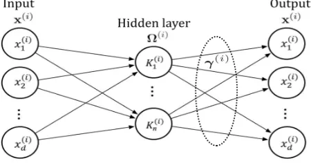
Fig. Architecture of the ith KELM-AE, in which the hidden layer A. KELM-AE
RBF with parameter σi in our case). In order to avoid confusion, Γ ̃ is used to represent the ith transformation matrix in KELM-AE, which can be learned similar to ELM-AE in Γ ̃
Ω(i) Γ ̃(i) = X(i)
Γ ̃(i)is calculated by
Γ ̃(i)= (I/C + Ω(i) )-1 X(i)
In the final step of transformation procedure, the data representation Xi+1 is obtained similar to
Xi+1 = g(X(i)(Γ ̃(i) )T)
where g is an arbitrary activation function. If the ith layer has the same dimension as the (i + 1)th layer, g can be
chosen as linear piecewise. In ML-KELM, all Γ ̃(i) (i>1) are of the same dimension n × n (i.e., square matrix). Then,
linear piecewise activation function can be applied to all Γ ̃(i), except Γ ̃(1) .
Hence, the transformation matrices Γ ̃(i) for i > 1 can be unified into a single matrix Γ ̃unified the representation
capability. Consequently, only two matrices Γ ̃(1) and Γ ̃unified can represent all transformations. KELM-AE is detailed
in Algorithm 1.
ML-KELM adopts two separate learning procedures as in H-ELM so that ML-KELM can also maintain the
universal approximation of ELM. In the stage of representation learning, each pair of Γ ̃(i) and X(i) (for ith KELM-AE)
can be calculated. Finally, the final data representation X final is calculated and fed as input to train a K-ELM classification model as follows:
Ω(final) β = T
where Ω(final) is the kernel matrix obtained from X(final) . The output weightβ is calculated by
β = (I/C + Ω(final))-1 T
Similarly, ML-KELM does not perform iterative fine-tuning once all the parameters are fixed in every layer. On the
other hand, the proposed ML-KELM does not need to tune Li , ai , and bi for any layer, which is a significant appeal
IV. RESULT AND DISCUSSIONS
In this section, ML-KELM is evaluated over 20 publicly available benchmark data sets from UCI repository and http://openml.org. All data sets are described in Table I and categorized into small, medium, and large in terms of size in order to have a thorough evaluation on the training time and testing accuracy.
A. Experiment Setup
The experiments are conducted using python 3.6 running on a 3.6-GHz i7 CPU with 16-GB RAM. The
number of hidden layers is set to 3 for all experiments. For ML-ELM and H-ELM, the numbers of hidden nodes Li (i =
1 to 3) are, respectively, set as 100 × m {m =, 2, . . . , 15}.
For the proposed ML-KELM, tuning of Li is not necessary and
RBF kernel is chosen as the kernel function for invertible
kernel matrix Ω. For all methods, the regularization parameter Ci (i = 1 to 3) in each layer is, respectively, set as 10 x ,
{x = −7, −5, . . . , 7}.
For ML-KELM, the kernel parameter σi (i = 1 to 3) in each layer is, respectively, set as 10 x {x = −7, −5, . . . ,
B. Evaluation of Testing Accuracy
For each of ML-ELM, H-ELM, and ML-KELM, the testing accuracy under the best combination of parameters is shown and compared in Table II, where ML-KELM outperforms the other two methods for all data sets (up to 7% for Pima). When there is plenty of data, ML-ELM performs similar to ML-KELM (Table II Large). However, ML-ELM
and H-ELM are suboptimal, because the input weight ai and bias bi in every layer are randomly generated. In some
cases, poorly generated ai and bi deteriorate the generalization of ML-ELM and H-ELM (shown in Table II). Therefore,
ML-ELM and H-ELM require numerous retrainings under fixed parameters in order to find out the best combination of
ai and bi for high model generalization. Furthermore, the accuracies of ML-ELM and H-ELM are very sensitive to Li .
C. Evaluation of Average Training Time
The average training times of ML-ELM, H-ELM, and ML-KELM are compared and shown in Table III. ML-KELM is the fastest for most of the small data sets. The reason is that the training time of ML-KELM depends on the number of
training data n, while ML-ELM and H-ELM depend on the number of hidden nodes Li . Subject to data complexity,
large Li tends to provide higher model generalization but increases training time. For small data sets, Li is usually larger
than n, so that ML-KELM is mostly with faster training time than ML-ELM and H-ELM. However, ML-KELM
becomes slower than ML-ELM and H-ELM in large data sets because of large n > Li. Nevertheless, in ML-ELM and
H-ELM, Li can easily become more than 10 000 for highly nonlinear applications (in our experiments, L i is set to at
most 1500, because the data are not highly nonlinear).
Although the average training time of ML-KELM becomes slower for large data sets, it is not the case practically. Note that Table III shows only the average training time for one model with fixed parameters. Although ML-ELM or
H-ELM take shorter average training time, they need to thoroughly try numerous combinations of parameters (such as Li ,
ai , and bi ) for the best model, so that ML-ELM or H-ELM may take even longer total training time. Even in the case
that thorough combinations of parameters are tried, ML-ELM or H-ELM may not have better model generalization than ML-KELM, due to the issue of accumulated reconstruction error (as shown in Table II). Therefore, it is more appealing to have a multilayer neural network with less user intervention, such as ML-KELM.
D. Evaluation on Highly Nonlinear Application
most 10 000 and the best combination of other parameters (e.g., network structure, regularization, scaling factors, kernel parameter, and so on) is experimentally determined for both ML-ELM and ML-KELM. The network structure of ML-ELM is (500-7000-2500-2) with regularization C and scaling factors (r ho, sig, and sig1) = 10 5 , 0.05, 0.7, 0.8, respectively, for layer 500-7000; 10, 0.05, 0.8, 0.9, respectively, for layer 7000-2500, and 10, 0.05, respectively, for layer 2500-2. On the other hand, for n = 2000, ML-KELM has an automatically determined structure
(500-2000-2000-2) with regularization C and kernel parameter σ set to 10 −7 , 10 −7 , respectively, for layer 500-2000; 10 3 , 10 5 ,
respectively, for layer 2000-2000, and 10 3 , 10 7 , respectively, for layer 2000-2. As shown in Table IV, ML-KELM significantly outperforms ML-ELM in terms of total training time, testing accuracy, and execution time. With kernel learning, ML-KELM can produce significant improvement on highly nonlinear applications.
V. CONCLUSIONS
In this brief, the proposed ML-KELM is a kernel version of ML-ELM by stacking multiple KELM-AEs, which has resolved several drawbacks over ML-ELM and H-ELM.
1) ML-KELM does not need to tune the parameters (Li , ai , and bi ) for all layers as in ML-ELM and
H-ELM.
2) ML-KELM learns an optimal model in one-shot under fixed parameters.
3) The transformation matrices Γ ̃(i) can be learned via exact inverse of kernel matrix rather than
pseudoinverse, resulting to better reconstruction of data representation and better model generalization. In the experiments, testing accuracy is improved up to 7% (for Pima).
4) Transformation matrices Γ ̃(i) for all layers can be combined into two transformation matrices only.
Their storage sizes are compact and fixed regardless to the number of hidden layers, which are helpful to those memory-critical systems. In addition, model execution time can be much shortened benefited from the unified transformation matrices.I
n a nutshell, ML-KELM has a remarkable improvement on the learning of data representation over ML-ELM and H-ELM with less user intervention.
REFERENCES
[1] Y. Bengio, “Learning deep architectures for AI,” Found. Trends Mach. Learn., vol. 2, no. 1, pp. 1–127, 2009.
[2] G. E. Hinton and R. R. Salakhutdinov, “Reducing the dimensionality of data with neural networks,” Science, vol. 313, no. 5786, pp. 504–507, 2006.
[3] L. J. P. van der Maaten, E. O. Postma, and H. J. van den Herik, “Dimensionality reduction: A comparative review,” J. Mach. Learn. Res., vol. 10, nos. 1–41, pp. 66–71, Oct. 2009.
[4] W. Wang, Y. Huang, Y. Wang, and L. Wang, “Generalized autoencoder: A neural network framework for dimensionality reduction,” in Proc.IEEE Conf. Comput. Vis. Pattern Recognit. Workshops, Jun. 2014,pp. 490–497.
[5] J. Deng, Z. Zhang, E. Marchi, and B. Schuller, “Sparse autoencoder-based feature transfer learning for speech emotion recognition,” in Proc. Humaine Assoc. Conf. Affective Comput. Intell. Interaction (ACII), Sep. 2013, pp. 511–516.
[6] P. Baldi, “Autoencoders, unsupervised learning, and deep architectures,”Unsupervised Transf. Learn. Challenges Mach. Learn., vol. 7, no. 1, pp. 37–50, 2012.
[7] C.-K. Shie, C.-H. Chuang, C.-N. Chou, M.-H. Wu, and E. Y. Chang, “Transfer representation learning for medical image analysis,” in Proc. 37th Annu. Int. Conf. IEEE Eng. Med. Biol. Soc. (EMBC), Aug. 2015, pp. 711–714.
[8] L. L. C. Kasun, H. Zhou, G.-B. Huang, and C. M. Vong, “Representational learning with extreme learning machine for big data,” IEEE Intell. Syst., vol. 28, no. 6, pp. 31–34, Nov. 2013.
[10] G.-B. Huang, Q.-Y. Zhu, and C.-K. Siew, “Extreme learning machine: A new learning scheme of feedforward neural networks,” in Proc. IEEE Int. Joint Conf. Neural Netw., vol. 2. Jul. 2004, pp. 985–990.
[11] J. Tang, C. Deng, and G.-B. Huang, “Extreme learning machine for multilayer perceptron,” IEEE Trans. Neural Netw. Learn. Syst., vol. 27, no. 4, pp. 809–821, Apr. 2016.
[12] G.-B. Huang, Q.-Y. Zhu, and C.-K. Siew, “Extreme learning machine: Theory and applications,” Neurocomputing, vol. 70, nos. 1–3, pp. 489– 501, 2006.
[13] S. Scardapane, D. Comminiello, M. Scarpiniti, and A. Uncini, “Online sequential extreme learning machine with kernels,” IEEE Trans. Neural Netw. Learn. Syst., vol. 26, no. 9, pp. 2214–2220, Sep. 2015.
[14] G.-B. Huang, H. Zhou, X. Ding, and R. Zhang, “Extreme learning machine for regression and multiclass classification,” IEEE Trans. Syst., Man, Cybern. B, Cybern., vol. 42, no. 2, pp. 513–529, Apr. 2012.
[15] I. Steinwart and A. Christmann, Support Vector Machines. New York, NY, USA: Springer, 2008.
[16] T. Greville, “The pseudoinverse of a rectangular or singular matrix and its application to the solution of systems of linear equations,” SIAM Rev., vol. 1, no. 1, pp. 38–43, 1959.
[17] K. He, X. Zhang, S. Ren, and J. Sun. (2015). Deep Residual Learning for Image Recognition. [Online]. Available: http://www.cvfoundation.org/openaccess/content_cvpr_2016/papers/He_Dee%p_Residual_Learning_CVPR_2016_paper.pdf
[18] C. Yan et al., “Efficient parallel framework for HEVC motion estimation on many-core processors,” IEEE Trans. Circuits Syst. Video Technol., vol. 24, no. 12, pp. 2077–2089, Dec. 2014.
[19] C. Yan, Y. Zhang, F. Dai, J. Zhang, L. Li, and Q. Dai, “Efficient parallel HEVC intra-prediction on many-core processor,” Electron. Lett., vol. 50, no. 11, pp. 805–806, 2014.
[20] C. Yan, Y. Zhang, F. Dai, X. Wang, L. Li, and Q. Dai, “Parallel deblocking filter for HEVC on many-core processor,” Electron. Lett., vol. 50, no. 5, pp. 367–368, Feb. 2014.
[21] M. Lichman, “UCI machine learning repository,” School Inf. Comput.Sci., Univ. California, Irvine, CA, USA, Tech. Rep., 2013. [Online]. Available: http://archive.ics.uci.edu/ml
[22] J. Vanschoren, J. N. Van Rijn, B. Bischl, and L. Torgo, “OPENML: Networked science in machine learning,” ACM SIGKDD Explorations Newslett., vol. 15, no. 2, pp. 49–60, 2014.
[23] B. Scholkopf and A. J. Smola, Learning With Kernels: Support Vector Machines, Regularization, Optimization, and Beyond. Cambridge, MA, USA: MIT Press, 2001.
[24] C. A. Micchelli, “Interpolation of scattered data: Distance matrices and conditionally positive definite functions,” Constructive Approx., vol. 2, no. 1, pp. 11–22, 1986.