| GENOMIC PREDICTION
Genomic Prediction Using Individual-Level Data and
Summary Statistics from Multiple Populations
Jeremie Vandenplas,*,1Mario P. L. Calus,* and Gregor Gorjanc†
*Wageningen University and Research, Animal Breeding and Genomics, 6700 AH, The Netherlands and†The Roslin Institute and Royal (Dick) School of Veterinary Studies, University of Edinburgh, Easter Bush Research Centre, Midlothian EH25 9RG, UK ORCID IDs: 0000-0002-2554-072X (J.V.); 0000-0002-3213-704X (M.P.C.); 0000-0001-8008-2787 (G.G.)
ABSTRACTThis study presents a method for genomic prediction that uses individual-level data and summary statistics from multiple populations. Genome-wide markers are nowadays widely used to predict complex traits, and genomic prediction using multi-population data are an appealing approach to achieve higher prediction accuracies. However, sharing of individual-level data across populations is not always possible. We present a method that enables integration of summary statistics from separate analyses with the available individual-level data. The data can either consist of individuals with single or multiple (weighted) phenotype records per individual. We developed a method based on a hypothetical joint analysis model and absorption of population-specific information. We show that population-specific information is fully captured by estimated allele substitution effects and the accuracy of those estimates,i.e., the summary statistics. The method gives identical result as the joint analysis of all individual-level data when complete summary statistics are available. We provide a series of easy-to-use approximations that can be used when complete summary statistics are not available or impractical to share. Simulations show that approximations enable integration of different sources of information across a wide range of settings, yielding accurate predictions. The method can be readily extended to multiple-traits. In summary, the developed method enables integration of genome-wide data in the individual-level or summary statistics from multiple populations to obtain more accurate estimates of allele substitution effects and genomic predictions.
KEYWORDSmeta-analysis; quantitative trait; statistical method; Genomic Prediction; GenPred; Shared Data Resources
G
ENOME-WIDE markers are nowadays widely used in animal and plant breeding to predict complex traits. This prediction is based on a linear model that partitions for each individual the observed complex phenotype value into systematic effects, comprising at least a population mean, an individual genetic value, and an environmental deviation (Fisher 1918). With genome-wide markers, indi-vidual genetic values can be computed from allele substitu-tion effects estimated from individual-level phenotype and genotype data (Meuwissenet al.2001). Subsequently, ge-netic values can be also computed for individuals of interest that are genotyped, but not phenotyped. This process iscommonly called genomic prediction. In animal and plant breeding, genetic values are used to identify genetically superior individuals and use them as parents of the next gen-eration to improve complex traits like milk yield (Meuwissen et al.2001; VanRaden 2008) or grain yield (Schulthesset al. 2016). In human genetics, genetic values can be used to dict individual genetic risk for complex diseases to inform pre-ventive and personalized medicine (de los Camposet al.2010; Wrayet al.2013; Pasaniuc and Price 2017).
Accuracy of estimated allele substitution effects and of resulting genetic values for complex traits are foremost a function of the number of individuals with available pheno-types and genopheno-types (Daetwyleret al.2008). To maximize the prediction accuracy, use of all available data are recom-mended (Henderson 1984; Wray et al.2013; Vilhjálmsson et al. 2015). In some small populations, collecting large amounts of data are not possible, and a joint analysis across multiple populations is needed to achieve high accuracy (Hozéet al.2014; Wientjeset al.2016). However, such joint analysis is often impossible, because of logistic or privacy
Copyright © 2018 by the Genetics Society of America doi:https://doi.org/10.1534/genetics.118.301109
Manuscript received May 3, 2018; accepted for publication July 16, 2018; published Early Online July 18, 2018.
Supplemental material available at Figshare: https://doi.org/10.25386/genetics. 6216533.
1Corresponding author: Wageningen University and Research, Animal Breeding and
considerations (Powell and Norman 1998; Maieret al.2018). Therefore, several methods were proposed to enable analysis of data from multiple populations when individual-level data are not available (Pasaniuc and Price 2017; Liu and Goddard 2018; Maieret al.2018). These methods, often called meta-analyses (Pasaniuc and Price 2017), approximate a joint analysis byfirst obtaining summary statistics from separate analyses of individual-level data for each population, and then combining these summary statistics to estimate genetic values. In human genetics, summary statistics usually con-sist of publically available allele substitution effects,i.e., genome-wide associations, together with their SE, esti-mated independently for each marker (Yanget al.2012; Vilhjálmssonet al.2015; Maieret al.2018). In livestock, summary statistics more likely consist of allele substitu-tion effects estimated jointly for all markers, together with prediction error (co)variances (Liu and Goddard 2018). While these methods may increase prediction accuracy in comparison to separate analyses, a loss in prediction ac-curacy is expected relative to an analysis using all individ-ual-level data due to approximations (Maieret al.2018). Further, these methods are based on some assumptions that make them difficult to apply outside their context of development. For example, Maieret al.(2018) implicitly assumed that only a single phenotype record per trait was associated with an individual. While this is usually the case in human genetics, it is not in breeding populations where individuals may have repeated phenotype records for the same trait, e.g., repeated longitudinal production or reproduction records in livestock or replicatedfield tri-als in crops, or when phenotype records are measured on a group of individuals and linked to a genotyped relative, e.g., progeny tested bulls for dairy production. Also, these developed methods do not allow combining individual-level data from some and summary statistics from other populations in one analysis (Liu and Goddard 2018; Maier et al.2018).
The objective of this study was to develop a method that jointly analyses individual-level data and summary statistics from multiple populations with no, or a limited amount of, approximation. The method assumes that individual-level data are composed of marker genotypes and phenotype re-cords that potentially have a variable number of replicates per individual. Further, summary statistics are assumed to be composed of estimated allele substitution effects with an associated measure of accuracy. Different measures of accu-racy can be used, which controls the amount of approxima-tion. The developed method is validated with simulated data. The results show that the method enables accurate integration of different sources of information across a wide range of settings.
Materials and Methods
Thefirst part of this section describes the theory of (1) sep-arate and joint analyses of two individual-level datasets,
(2) an exact integration of estimated allele substitu-tion effects from one populasubstitu-tion into the analysis of another, (3) approximate integrations, and (4) general-ization for multiple populations. The second part de-scribes simulations used for validation of the developed method.
Theory
Assume we have two populations with independent individual-level datasets of phenotyped and genotyped individuals. The two populations and their corresponding datasets are hereafter referred to as 1 and 2. Further assume that both datasets contain the same markers. From this data we want to obtain accurate estimates of allele sub-stitution effects and genetic values for complex traits. We can achieve this by a joint analysis of the two datasets. When one of the datasets is not available, we can achieve this by integrating the results of a separate analysis of the un-available data into the separate analysis of the un-available dataset. We show how to perform this integration exactly or approximately.
Separate and joint analyses: A standard marker model, using random regression on marker genotypes, for the sepa-rate analysis of dataseti(i= 1, 2) is:
yi¼Xib*
i þZiWiai*þe
*
i; (1)
whereyiis anobs;i31 vector of phenotypes,b*
i is anf;i31
vector of fixed effects that are linked to yiby a nobs;i3nf;i incidence matrixXi,ai*is anmar31 vector of allele
substitu-tion effects that are linked to yi by anobs;i3nind;iincidence
matrixZiand anind;i3nmarmatrix of genotypesWi;ande*
i is
the vector nobs;i31 of residuals. In this work we consider
single-nucleotide polymorphism markers, which we code in Wias 0 for homozygous aa, 1 for heterozygous aA or Aa, and
2 for homozygous AA. Other genotype coding and centering, that is of the formðWi1v
0
iÞwith 1 being anind;i31 vector of
ones and vi being a nmar31 vector, can be used with no
difference in obtained estimates of allele substitution effects (Strandén and Christensen 2011). We assume a prior multi-variate normal (MVN) distribution for allele substitution ef-fects for the separate analysis of the dataseti,a*i, with mean
zero and covarianceBis2ai;a*i MVNð0;Bis
2
aiÞ;whereBiis a
nmar3nmardiagonal matrix (e.g., an identity matrixI), and s2
ai is the variance of allele substitution effects. We also as-sume that residuals are multivariate normally distributed with mean zero and covariance Ris2e; e*i MVNð0;Ris2eÞ;
whereRiis anobs;i3nobs;i diagonal matrix (e.g., an identity
matrix I), and s2
e is the residual variance. For simplicity,
and without loss of generality, it is assumed in the follow-ing that residual variances are the same for all separate and joint analyses. Variance componentss2
ai ands2e are
Meuwissenet al.2001; de los Camposet al.2012) with op-tional different weights inBi(to differentially shrink different
loci) andRi(to account for heterogeneous residual variance
due to variable number of repeated phenotype records per individual).
Separate estimates of allele substitution effects ca*i are
obtained by solving the following system of equations:
"
X9
iR2i 1s2e2Xi Xi9R2i 1s2e2ZiWi W9
iZ9iR2i 1se22Xi W9iZ9iR2i 1s2e2ZiWiþB2i 1s2ai2
# cb*
i c ai* ¼ X9
iR2i1s2e2yi W9iZ9iR2i 1s2e2yi
:
(2)
Separate estimates of genetic values for individuals in a data-seti(i= 1, 2) are obtained bygb*
i ¼Wica*i:
A marker model for the joint analysis of two datasets 1 and 2 is:
y1 y2 ¼
X1 0 0 X2
b1 b2 þ
Z1W1 Z2W2
aþ e1 e2 ; (3)
where phenotypes from the two populations are modeled with population-specific fixed effects ðb1;b2Þ; but a joint set of allele substitution effectsðaÞ:We assume a MVN prior distri-bution for allele substitution effects with mean zero and co-varianceBJs2aJ;aMVNð0;BJs2aJÞ;whereBJis anmar3nmar
diagonal matrix, and s2
aJ is the variance of allele substi-tution effects in the joint analysis. We also assume that re-siduals are multivariate normally distributed, specifically
e1 e2
MVN 00
;
R1 0 0 R2
s2
e !
where Ri is a
nobs;i3nobs;idiagonal matrix.
Joint estimates of allele substitution effectsa^are obtained by solving the following system of equations:
Joint estimates of genetic values for individuals in a dataseti (i= 1, 2) are obtained bygbi¼Wia^:
Exact integration: The integration of estimates of allele substitution effects from one dataset into the analysis of another can be performed by means of absorbing cor-responding equations in the joint system of equations. We choose to integrate estimates from the dataset 1 into the analysis of dataset 2. Derivations in Appendix A1 lead to the following system of equations that performs such in-tegration and gives equivalent estimates of allele substitu-tion effects to the joint analysis (Eq. 4):
where ac*1 are estimates of allele substitution effects from the separate analysis of dataset 1 using (Eq. 2), and
PECca1*
21
is the inverse of the corresponding predic-tion error covariance (PEC) matrix. The latter can be
obtained as
PECca1*
21
¼W9
1Z91M1se22Z1W1þB2 1 1 s2a12
with M1¼ ðR2112R2 1
1 X1ðX91R2 1 1 X1Þ
21 X9
1R2 1
1 Þ. Note that only the individual-level dataset 2 and summary statistics from the dataset 1 (i.e., the estimated allele substitution effects and their PEC) are required. Individual-level data-set 1 is therefore not required.
It is worth noting that the integration of estimates of allele substitution effects from the dataset 1 into the analysis of dataset 2 can also be obtained from a Bayesian context. Bayes estimators for linear mixed models were discussed by several authors (Lindley and Smith 1972; Dempfle 1977; Gianola and Fernando 1986). In a Bayesian context, we can assume the following prior multivariate normal distributions for the marker model (Eq. 1) applied to dataset 2:
2 4 X
9
1R211s2e2X1 0 X91R211s2e2Z1W1
0 X9
2R221s2e2X2 X29R221s2e2Z2W2 W9
1Z91R211s2e2X1 W92Z29R221s2e2X2 W91Z91R211s2e2Z1W1þW92Z92R221s2e2Z2W2þB2J1s2aJ2
3 5 2 4 c b1 c b2 ^ a 3 5¼ 2 4 X 9
1R211s2e2y1 X9
2R221s2e2y2 W9
1Z91R211s2e2y1þW92Z92R221s2e2y2
3 5
(4)
" X9
2R221s2e2X2 X29R221s2e2Z2W2 W9
2Z92R221s2e2X2
PECca1* 21
þW9
2Z92R221s2e2Z2W22B211s2a12þB 21
J s2aJ2 #" c b2 ^ a # ¼ " X9
2R221s2e2y2
PECca1* 21
c
a1*þW92Z92R221s2e2y2 #
h
b* 2 jb2;U2
i
MVNðb2;U2Þ;
whereb2is a mean vector andU2is a (co)variance matrix,
h
a* 2
B2s2a2
i
MVN0;B2s2a2
; and h e* 2 R2s2
e
i
MVN0;R2s2e
:
Assuming a noninformative prior forb*
2;the system of equa-tions (2) for dataset 2 can be obtained by differentiating the joint posterior distribution ofb*
2 anda*2 with respect tob*2 anda*
2;and setting the derivatives equal to 0 (Gianola and Fernando 1986). Integration of estimates of allele substitu-tion effects from dataset 1 into the analysis of dataset 2 can be therefore obtained by defining a MVN prior distribution for allele substitution effects in the analysis of dataset 2 using the posterior distribution for allele substitution effects from a separate analysis of dataset 1:
h
aca1*;PECa1c*;B1s2 a1;BJs
2 aJ
i
MVNQPECca1*21a1c*;Q;
(6)
Q¼
PECac1*
21
2B21
1 s2a12þB
21
J s2aJ2
!21
:
The matrix Q can be considered as the PEC matrix of a hypothetical separate analysis of dataset 1 using the MVN prior distribution for allele substitution ef-fects of the joint analysis, that is a1*MVNð0;BJs2aJÞ and Q¼W91Z91M1se22Z1W1þB2J1s2aJ2
21
;and the vector
Q PECca1*
!21
c
a1* can be considered as the estimated
allele substitution effects of this hypothetical separate anal-ysis. In animal breeding, a similar approach was used to integrate estimated genetic values and associated accura-cies from one genetic evaluation into another genetic evalua-tion (Quaas and Zhang 2006; Legarraet al.2007; Vandenplas and Gengler 2012).
Finally, it is worth noting that the termPECca1*
21
c
a1* can be interpreted as a vector of hypothetical or pseudophe-notype records associated with allele substitution effects, and, as such, summarize available information in dataset 1. In this sense, the system (Eq. 5) is similar to approaches that compute pseudorecords associated with individuals, from available estimated genetic values where individual-level phenotypic information is not readily available, or is not measured on the individuals themselves but on close relatives. In animal breeding, these approaches are com-monly known as deregression of estimated genetic values (Jairathet al.1998).
Approximate integration:Exact integration requires the in-verse of PEC matrix from the separate analysis, which could be approximated when unavailable. Genomic analyses of com-plex traits that combine different datasets commonly have access to estimated allele substitution effects and associated prediction error variances (in different forms), but not the whole PEC matrixPEC
c
a1*
required in (5). We propose sev-eral ways to accommodate this situation. We assume that we know, at least, the prediction error variances (PEV) of esti-mated allele substitution effectsPEVca*1
;the number of individuals ðnind;1Þ; and variance components used in the separate analysis of dataset 1 (s2
a1ands
2
e).
When only the PEV of the estimated allele substitution
effects
PEV
c
a1*
are known, while PEC are not, then we
can approximatePECca1*
21
withPEVca1*
21
:This ap-proximation would be accurate if the matrix productW91W1 has (close to) zero off-diagonal elements, which is dependent on the characteristics of genotypes in dataset 1 (e.g., allele frequencies, linkage disequilibrium (LD), and population/ family structure). If this is not the case, the approximation will bias the analysis by ignoring off-diagonal elements.
When allele frequencies and LD correlations in data-set 1 are known, we can obtain a good approximation of PECac*1
under some conditions (one phenotype record per individual, homogenous residual variance, overall mean is the onlyfixed effect, and Hardy-Weinberg equilibrium). Deri-vations in Appendix A2 show that, under these conditions, we can approximate PECca1*
with ðW91W1s2e2þB2
1 1 s2a12Þ
21
with the unknown matrix W91W1 approximated from commonly available population parameters (i.e., allele fre-quencies and LD correlation) as 4nind;1pp9þV
1
2CV12;where
pis anmar31 vector of allele frequencies,Vis anmar3nmar diagonal matrix of expected genotype sum of squares with thei-th diagonal element equal tonind;12pi;1ð12pi;1Þ, andC is anmar3nmarmatrix of pairwise genotype correlations
be-tween markers. In practice, the matrixCfor dataset 1 could be unknown, but we can approximate it by using a reference panel that includes, for example, available genotypes of non-phenotyped individuals originating from this population (Yanget al.2012; Vilhjálmssonet al.2015; Maieret al.2018). Finally, we relax the assumption of having a single pheno-type record per individual in the preceding approximations. This is relevant when individuals have repeated phenotype records,e.g., repeated longitudinal production or reproduc-tion records in livestock or replicatedfield trials in crops. A related issue is the violation of assumption of homogenous residual variance when phenotype records arefirst prepro-cessed and then used in genomic analyses,e.g., deregressed progeny proofs in livestock (e.g., Garricket al.2009) or ad-justed field trial means in crops (e.g., Schulz-Streeck et al. 2013; Oakey et al. 2016; Damesa et al. 2017). For these situations, we show in Appendix A3 that we can approximate
PECac*1
with L1
4pp9þC1 2CC12
L1s2e2þB2
1 1 s2a12
21
where C is anmar3nmar diagonal matrix with thej-th
di-agonal element equal to 2pj;1ð12pj;1Þ, and L1 is a nmar3nmar diagonal matrix with thej-th diagonal element
representing the square root of effective number of records for thej-th marker. The matrixL1can be obtained by solving the nonlinear system of equations
diag L14pp9þC12CC 1 2
L1s22
e þB211s2a12 21!
¼PEVa1c*
through afixed-point iteration algorithm (Burden and Faires 2010) detailed in Appendix A3. It is worth noting that the proposed algorithm requires the inversion of a nmar3nmar
dense matrix at each iteration. This computational cost can be reduced by performing the algorithm for each chromo-some separately.
Integration with multiple populations: When more than two populations or datasets are available, the developed methods can be easily extended. With ndatasets, the prior distribution for allele substitution effects in the separate anal-ysis of then-th dataset is defined using the posterior distri-butions for allele substitution effects from the separate analyses ofn21 datasets:
" aca1*;ca*
2;. . .;ad*n21 #
MVN QX
n21
i¼1
PECca*i
21 c a*i
;Q
! ;
Q¼ B21
J s2aJ2þ
X
n21
i¼1
PEC
c
ai*2 1
2B21
i s2ai2
!21
:
Simulations
We tested developed methods with simulated data that either had low or high genetic diversity. The data were simulated in
five replicates with the AlphaSim program, which uses the coalescent method for simulation of base population somes and the gene drop method for simulation of chromo-some inheritance within a pedigree (Hickey and Gorjanc 2012; Fauxet al.2016).
A diploid genome was simulated with 30 chromosomes, each 108bp long. Coalescent mutation and recombination rate per base pair were set to 1028, while effective population size was modeled over time to mimic population history of a livestock population in line with the values reported by MacLeodet al.(2013). Specifically, for the low diversity sce-nario, the effective population size of the base population was set to 100 and increased to 120, 250, 350, 1000, 1500, 2000, 2500, 3500, 7000, 10,000, 17,000, and 62,000 at, respec-tively, 6, 12, 18, 24, 154, 454, 654, 1754, 2354, 3354, 33,154, and 933,154 generations ago. For the high diversity scenario, effective population size of the base population was set to 10,000 and increased above this value in the same way as in the low diversity scenario; to 17,000 and 62,000 at 33,154, and 933,154 generations ago. For each chromosome,
10,000 whole chromosome haplotypes were sampled, which, on average, hosted 700,000 markers (21 million per ge-nome) for the low diversity scenario and 1,400,000 markers (42 million per genome) for the high diversity scenario. Out of these loci, 100 per chromosome (3000 per genome) were sampled as causal loci affecting a complex trait. The allele substitution effect of causal loci was sampled from a normal distribution with mean zero and variance 1/3000. The effects were used to simulate a complex trait with additive genetic architecture. In addition, 2000 loci per chromosome (60,000 per genome) were selected as markers with the restriction of having minor allele frequency above 0.05.
From the base population, founder genomes for four pop-ulations (A, B, C, and D) were obtained by random sampling of chromosomes with recombination. The populations were ancestrally related through the common base population, but otherwise maintained independently,i.e., there was no migration between the four populations. Each population was initiated with 10,000 founders (half males and half fe-males) and maintained for seven generations with constant size. In the low diversity scenario, with the effective popula-tion size of 100, 25 males and 5000 females were selected as parents of each generation, while in the high diversity scenario, with the effective population size of 10,000, all 5000 males and 5000 females were used. The 25 males were selected on true genetic value, assuming accurate progeny test was available.
For every individual in the population we simulated two types of phenotypes. First, an own single phenotype was simulated as the sum of the true genetic value and a residual sampled from a normal distribution with mean zero and residual variance scaled relative to the variance of true genetic value in the base population such that heritability was 0.3. These simulated single phenotype records mimic records measured on the individual. Second, a weighted phenotype was simulated as the sum of the true genetic value and the mean ofnweightresiduals. Each residual was sampled from a
normal distribution with mean zero and residual variance scaled relative to the variance of true genetic value in the base population such that heritability was 0.3. The weight nweightwas equal tonweight ¼1þvalwhere the real valueval
was sampled from a geometric distribution with a probability pof 0.15 and a probability mass function ofPrðxÞ ¼pð12pÞx withx2 f0; 1; 2;. . .g. The averagenweightwas 6.6. These
weighted phenotypes mimic either repeated records of an individual or records on multiple progeny of an individual. To satisfy the assumption of identical residual variance across all analyses, phenotype records were divided by the residual SD specific for each population, such thats2
e ¼1. For every
individual in each population we stored the true genetic value, own single and weighted phenotype records, associ-ated weight, and 60,000 marker genotypes.
Analysis
genetic values utilizing all the available information. Specifi -cally, we integrated results from separate analysis of popula-tions B, C, and D, into the analysis of population A. We assumed throughout that variance components were known and equal to the rescaled variances. We analyzed three scenarios in total. Thefirst and second scenario used population specific training data of randomly sampled 30,000 individuals with single phenotype record from generations 1–6 under low and high diversity settings. The third scenario used population specific training data of randomly sampled 10,000 individuals with weighted phenotype record from generations 1–6 under low diversity setting. In all scenarios all of the 10,000 individuals from generation 7 of each population were considered as val-idation individuals. The following analyses were performed:
1. A joint analysis of four populations. This was the reference that the other analyses were compared against;
2. A separate analysis for each of the four populations; 3. An exact integration of separate analyses of populations B,
C, and D, into the analysis of population A;
4. The same as 3, but approximating the PEC matrix with a partial PEC matrix for each chromosome,i.e., PEC between markers on different chromosomes were set to zero; 5. The same as 3, but approximating the PEC matrix with a
diagonal PEV matrix,i.e., PEC between all markers were set to zero;
6. The same as 3, but approximating the PEC matrix with PEV, allele frequencies, and LD correlations between markers ob-tained from the training sets. For the scenario with weighted phenotype records, the algorithm for estimating the effec-tive number of records per marker was performed for each marker separately and for each chromosome separately. 7. The same as 6, but with LD correlations between markers
computed from validation individuals instead of the train-ing data.
For each analysis we calculated genomic prediction accu-racy as the Pearson correlation between the true and esti-mated genetic value in validation individuals. Further, we evaluated the different integrations by comparing estimated genetic values of validation individuals against the estimated genetic values obtained from the joint analysis, which was considered as the reference because it used information from all populations. If integration was fully accurate, there should be no difference between the joint analysis and the analysis with integration. We assessed this by (a) accuracy of integra-tion as a Pearson correlaintegra-tion between estimated genetic values from the joint analysis and the analysis with integration (desired value equals 1), (b) calibration of integration as a regression of estimated genetic values from the joint analysis on estimated genetic values from analysis with integration, and (c) magnitude of error in integration as a mean square error (MSE) between estimated genetic values from the joint analysis and from the analysis with integration (desired value equals 0). By calibration, we mean the slope of relationship of the estimates from the integration analysis onto the estimated genetic values from the joint analysis. The desired slope value
is 1, which indicates a well calibrated model. Values above or below 1 indicate an uncalibrated model.
Data availability
Supplementalfigures are available in Supplemental Material, File S1. A description of the simulated genotype and pheno-type datasets for each scenario is provided in File S2. Simu-lated genotype and phenotype datasets for thefive replicates of each scenario are provided in Files S3–S5. Data simulation scripts and Fortran codes developed to perform the different analyses, as well as a short description of each of them, are provided in File S6. Supplemental material available at Fig-share:https://doi.org/10.25386/genetics.6216533.
Results
Genomic prediction accuracy of separate and joint analyses
Joint analysis increased genomic prediction accuracy in com-parison to separate analyses. This is shown in Table 1. Ana-lyzing separately the four datasets gave accuracies of0.71 (low diversity) and 0.53 (high diversity) with single pheno-type records, and of 0.73 (low diversity) with weighted phenotype records. Analyzing jointly the four datasets in-creased accuracy by at least 0.09 absolute points with single phenotype records and by at least 0.12 absolute points with weighted phenotype records.
Integration based on PEC, partial PEC, or PEV matrices
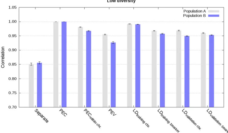
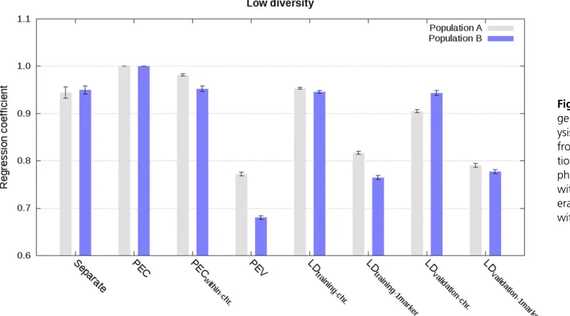
For all scenarios, the developed method enabled exact in-tegration when complete PEC matrices were used. Inin-tegration of estimated allele substitution effects by means of the com-plete PEC matrix led to the same estimated genetic values as with the joint analysis, as shown by correlation and regres-sion coefficients of 1, and MSE close to 0 (Figure 1, Figure 2, Figure 3, Figure 4, and Figures S1–S8). For comparison, correlations between estimated genetic values from sepa-rate analyses and joint estimated genetic values were0.87 (low diversity) and 0.77 (high diversity) with single type records, and 0.85 (low diversity) with weighted pheno-type records.
Table 1 Genomic prediction accuracy for joint and separate analyses in scenarios with single or weighted phenotype records and low or high diversity (values are averages across the five replicates)
Phenotypesa Diversity Analysis Populations
A B C D
Single Low Joint 0.811 0.811 0.823 0.815
Approximate integration by means of partial PEC matrices for each chromosome, that is ignoring PEC between markers on different chromosomes, gave almost as accurate and cali-brated estimated genetic values as the exact integration. This is illustrated in Figure 1, Figure 2, Figure 3, Figure 4, and Figures S1–S8 with correlations higher than 0.96, regression coefficients close to 1, and MSE close to 0. Increasing the diversity slightly deteriorated accuracy and calibration of ge-nomic predictions (Figure 1, Figure 2, and Figures S1–S4).
Approximate integrations by means of PEV matrices, that is ignoring PEC between all markers, gave quite accurate, but not calibrated estimated genetic values. This is shown in Figure 1, Figure 2, Figure 3, and Figure 4 and in Figures S1–S8. Correla-tions between joint estimated genetic values and estimated ge-netic values with integration by means of PEV were between 0.95 and 0.98 with single phenotype records and between 0.93 and 0.95 with weighted phenotype records. Despite these correlations close to 1, estimated genetic values were not well calibrated, as depicted by regression coefficients below 0.77 for the low di-versity scenarios with single and weighted phenotype records, and below 0.86 for the high diversity scenario with single phe-notype records (Figure 2, Figure 4, and Figures S2 and S6).
Integration based on PEV, allele frequencies, and LD information
When LD information was derived from training data of other populations, approximate integrations by means of PEV, allele frequencies, and LD information, resulted in highly accurate and well calibrated estimated genetic values with single
phenotype records. This is shown in Figure 1 and Figure 2 (Figures S1–S4). Correlation and regression coefficients were equal to 1 for the low diversity scenario. Slightly lower values, but still close to 1, were observed for the high diversity sce-nario. For both low and high diversity scenarios, MSE were close to 0. In contrast, when LD information was derived from validation data of other populations, approximate integrations gave less accurate and calibrated estimated genetic values. This is shown in Figure 1 and Figure 2 (Figures S1–S4). For these scenarios, correlations were equal to at least 0.94, and regression coefficients varied between 0.87 and 1.05.
reduced accuracy and calibration of estimated genetic values (Figure 3, Figure 4, and Figures S5 and S6).
Comparison of estimated allele substitution effects
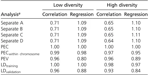
Correlation and regression coefficients between estimated allele substitution effects from the joint analysis and analysis with integration largely followed patterns of the correspond-ing values for estimated genetic values (Table 2 and Table 3). Correlation and regression coefficients were close to 1 when
the integration of estimated allele substitution effects was by means of the complete PEC matrices. Ignoring PEC between markers on different chromosomes, or ignoring PEC between all markers, reduced correlations to between 0.92 and 0.99 (Table 2 and Table 3). Using LD information with PEV led to correlations between joint estimates of allele substitution ef-fects and estimates with integration ranging from 0.71 to 0.83 for the scenario with weighted phenotype records (Ta-ble 2 and Ta(Ta-ble 3).
Discussion
The results show that the developed method enables accurate and well-calibrated estimated genetic values for complex traits using both individual-level data and summary statistics. As expected from theory, the analysis of individual-level data and estimated allele substitution effects from other analyses by means of PEC matrices, yielded the same estimates as the joint analysis of all individual-level data. To our knowledge, this is thefirst time that individual-level data and summary statistics were analyzed simultaneously for genomic predic-tions. As illustrated by simulations, the combined analysis of multiple datasets may increase genomic prediction accuracy over separate analyses of a single dataset. Unfortunately, combining individual-level data from several sources is gen-erally not feasible for several reasons, e.g., political road-blocks, data protections concerns, or data inconsistencies (Powell and Sieber 1992; Vilhjálmsson et al. 2015; Maier et al.2018). However, summary statistics, such as estimates of allele substitution effects and associated measures of ac-curacy (e.g., PEV), are usually available for exchange in hu-man genetics, or are discussed to be shared, e.g., at an international level for dairy cattle breeding (Liu and Goddard 2018). The developed method enables increase in genomic prediction accuracy of complex traits by means of jointly an-alyzing the available individual-level data and summary statistics.
Accurate integration of estimated allele substitution effects is possible also when the complete PEC matrix is not available. This is important because computing the exact PEC matrix and exchanging it between analyses might be challenging in some cases. For the vast majority of marker arrays used in animal and plant breeding, the calculations and data transfers should be doable. For example, most arrays have between 10,000 and 100,000 markers, for which we need between1 and
80 GB of memory to store the PEC matrix and between a minute and a day to invert it on current computers. For a larger number of markers, commonly used in human genet-ics, the memory requirements and computing time become prohibitive. The results show that in such cases we can still obtain accurate genomic predictions when the integration is done by means of partial PEC matrices for each chromosome. This is expected since high LD between markers mostly occurs within chromosomes. High LD between markers on different chromosomes may especially occur in structured populations and populations under selection (Farnir et al. 2000; Flint-Garciaet al.2003; Rostokset al.2006). Both of these conditions are present in breeding populations. How-ever, the results suggest that LD between chromosomes can be ignored for the purpose of integration for populations with both low and high diversity. The results also show that we can successfully integrate estimated allele substitution effects when only PEV and allele frequencies from each population are available together with LD information of a reference genotype panel representative of each population. Assuming that such reference genotype panels are available, only esti-mated allele substitution effects, associated PEV, and allele frequencies need to be exchanged between populations for such analyses. Similar conclusions were drawn from studies combining only summary statistics obtained from genome-wide association studies to perform multi-trait genomic pre-dictions (Maieret al.2018).
LD and allele frequency information), whatever the level of diversity and characteristics of the populations, as shown by our results or a study combining summary statistics in human genetics (Maier et al. 2018). In our study, the population parameters obtained from the reference panels adequately reflected the characteristics of the training sets. We expect that this would be the case for populations with substantial migration, such as, for example, Holstein dairy cattle popu-lations. Future studies should be conducted to assess the impact of suboptimal reference panels. Therefore, the devel-oped method is expected to perform well on any type of data, from animal and plant breeding to human genetics, provided accurate information is available.
The developed method has some simplifying assumptions that can be readily relaxed. For example, we assumed that the same genotype coding was used in all populations. This as-sumption can be relaxed when centered genotype coding (i.e., of the form ofðWi1v
0
iÞ) is used because variance component
estimates, estimates of allele substitution effects and PEC are the same irrespective of the centering of the genotype coding, provided that the model has afixed general mean, which is considered in the integration (Strandén and Christensen 2011). Also, centered and scaled (standardized) genotype coding is often used in human genetics, instead of only centered genotype coding (Yang et al. 2010; Speed et al. 2012; Maier et al. 2018). In practice, estimates of genetic values are only slightly influenced by scaling of centered genotype coding (Strandén and Christensen 2011; Bouwman et al. 2017). Therefore, assuming that the same estimated genetic values are obtained with different scaling, allele substitution effects estimated using one type of genotype scaling could be obtained from a postanalysis by converting estimated genetic values computed for a reference genotype panel into allele substitution effects for another genotype scaling. Converting estimated genetic values into allele substitution effects is often referred to as back-solving of allele substitution effects (Strandén and Garrick 2009; Strandén and Christensen 2011; Wanget al.2012; Bouwmanet al.2017). PECs associ-ated with the converted estimassoci-ated allele substitution effects
could be derived from the (prediction error) covari-ances of the estimated genetic values (see derivations in Ap-pendix A4).
Allele substitution effects estimated from analyses using different sets of markers or different residual variances, can be used in the integration as well. The assumption that all individuals were genotyped at the same loci could be consid-ered as fulfilled if small differences in the sets of markers are corrected by assuming zero allele substitution effect and zero accuracy for markers not used in an analysis. When large differences between sets of markers are observed, this assump-tion can be accommodated following two approaches. Afirst, postanalysis, approach consists of assuming that estimated genetic values are the same for two different sets of markers, allowing the conversion of estimated allele substitution effects from one set of markers to another set of markers (Liu and Goddard 2018). The conversion can be performed by back-solving estimated allele substitution effects from estimated ge-netic values, as proposed previously for different genotype codings, or by applying a marker model to the estimated ge-netic values with the reference set of markers (Liu and God-dard 2018). A second approach consists of harmonizing genotype data across populations. This approach must be per-formed before the analyses, and requires therefore coordina-tion between populacoordina-tions. Harmonizacoordina-tion of genotype data could be performed by identifying a subset of markers for which all populations are genotyped, or by genotype imputa-tion (e.g., Marchini and Howie 2010). Finally, the assumption that residual variances were the same in all populations, can be relaxed by noting that separate estimates of allele substitution effectsca*
i;obtained by the system of equations (2), can be also
obtained by the following different formulations:
c
ai*¼W9
iZ9iMis2eiZiWiþB 21
i s2ai2
21
W9
iZ9iMis2eiyi ¼W9
iZ9iMiZiWiþB2i 1l
21
W9 iZ9iMiyi
¼W9
iZ9iMis2ef2ZiWiþB 21
i ls2ef2
21
W9
iZ9iMis2ef2yi Table 3 Comparison of estimated allele substitution effects from different analyses with estimates from the joint statistical analysis using weighted phenotype records in the scenario with low diversity (values are averages across thefive replicates with SE between brackets)
Analysis Correlation Regression
Separate A 0.61 (0.10) 0.88 (0.13)
Separate B 0.58 (0.15) 0.62 (0.12)
Separate C 0.56 (0.12) 0.93 (0.23)
Separate D 0.33 (0.08) 0.65 (0.18)
PEC 1.00 (0.00) 0.99 (0.01)
PECwithin chromosome 0.96 (0.01) 1.01 (0.02)
PEV 0.92 (0.02) 0.80 (0.05)
LDtraining(1 marker) 0.77 (0.09) 0.83 (0.10)
LDtraining(1 chromosome) 0.83 (0.09) 0.95 (0.11)
LDvalidation(1 marker) 0.73 (0.11) 0.75 (0.13)
LDvalidation(1 chromosome) 0.71 (0.15) 0.74 (0.18)
Table 2 Comparison of estimated allele substitution effects from different analyses with estimates from the joint statistical analysis using single phenotype records in scenarios with low and high diversity (values are averages across thefive replicates)
Analysisa
Low diversity High diversity
Correlation Regression Correlation Regression
Separate A 0.71 1.09 0.65 1.10
Separate B 0.71 1.09 0.65 1.10
Separate C 0.71 1.09 0.65 1.11
Separate D 0.71 1.09 0.64 1.10
PEC 1.00 1.00 1.00 1.00
PECwithin chromosome 0.99 0.98 0.97 0.95
PEV 0.96 0.80 0.96 0.89
LDtraining 1.00 1.00 0.98 0.97
LDvalidation 0.96 0.88 0.93 0.84
wheres2
ei
s2
ef
is the residual variance used for thei-th (fo-cal) analysis, andl¼s2
eis 22 ai :
For integration of ca*i; PEC
c
a*i
21
must be
approxi-mated using the residual variance of the focal population (s2ef) and the effective numbers of records per marker es-timated using variance components of the i-th analysis. Another way to relax this assumption is to extend our uni-variate model to a biuni-variate model, similarly to methods de-veloped to combine different genetic evaluations in animal breeding (Schaeffer 1994; Vandenplaset al.2015). In a bi-variate model, one trait would represent individual-level data, while the other trait would represent summary statis-tics. The genetic correlation between the two traits could be estimated based on a subset of individual-level data available for both datasets or based on summary statistics (Bulik-Sullivan et al.2015). Such an approach would also allow the integra-tion of summary statistics expressed on a different scale (e.g., different measure units, trait definitions) than the scale of the focal population (Vandenplaset al.2015).
The developed method can be readily generalized to multi-trait models and is therefore a generalization of previous works that were based on several (implicit) assumptions (Liu and Goddard 2018; Maier et al. 2018). For example, previous works assumed that no individual-level data were available. It was also (implicitly) assumed that only single phenotype records with homogeneous residual variance (Maieret al.2018), or that the least-squares part of the sep-arate analyses (Liu and Goddard 2018), were available for integrating estimated allele substitution effects. Both as-sumptions lead to simple and accurate approximations of PEC matrices as shown in our study. However, we relax all these assumptions, such that our method can jointly analyze individual-level data and summary statistics, with possibly multiple phenotype records per individual.
With all the proposed generalizations, the developed method could be used in different contexts. For example, in human genetics, allele substitution effects with associated SE are publicly available (Yang et al.2012; Vilhjálmssonet al. 2015; Maier et al. 2018). In animal breeding, individuals9 genetic values with associated reliabilities are publicly avail-able and in the case of dairy cattle extensively combined across multiple populations (Schaeffer 1994; VanRaden and Sullivan 2010; Jorjani et al. 2012; Vandenplas et al. 2017). The developed method can be used in both contexts, but, in the latter case, individuals9genetic values must befirst back-solved to allele substitution effects (Strandén and Garrick 2009; Strandén and Christensen 2011; Wanget al.2012; Bouwmanet al.2017). It is worth noting that our method assumes that summary statistics from one population are free of information from other populations. This suggest that it can be used when there is no, or limited, sharing of informa-tion between populainforma-tions, as is, for example, the case in beef cattle, but not in dairy cattle populations such as Holstein, where pseudophenotypes summarizing information from
multiple populations are used extensively (VanRaden and Sullivan 2010; Jorjani et al.2012). This assumption can be relaxed by performing separate analyzes free of information from other populations, or by correcting for double-counting of information, which has bee developed for the integra-tion of estimated genetic values from different populaintegra-tions (Vandenplaset al.2014, 2017; VanRadenet al.2014). This correction for double-counting of information is not yet de-veloped for the integration of summary statistics, and should be investigated in future studies.
Conclusions
We developed a method for genomic prediction that accurately integrates summary statistics obtained from analyses of separate populations into an analysis of individual-level data. The method accommodates use of multiple phenotype (pseudo)records per individual, and further extensions have been presented to accommodate for differences in residual variances or genotype codings used in the populations. When complete summary statistics information is available the method gives identical genomic predictions as the joint analysis of individual-level data from all populations. When summary statistics information is not complete we can use a series of approximations that give very accurate and well-calibrated genomic predictions.
Acknowledgments
This study was financially supported by the Dutch Ministry of Economic Affairs (TKI Agri & Food project 16022), the Breed4Food partners Cobb Europe, CRV, Hendrix Genetics and Topigs Norsvin, and United Kingdom Biotechnology and Biological Sciences Research Council (BBSRC) Institute Stra-tegic Programme Grant (ISPG) to The Roslin Institute BBS/ E/D/30002275. The use of the high performance computing (HPC) cluster has been made possible by CAT-AgroFood (Shared Research Facilities Wageningen University and Research).
Author contributions: J.V. derived the equations, wrote the programs to do the analyses, performed the analyses, and drafted the outline of the manuscript. G.G. performed the simulations. All authors discussed the design of the simula-tions. J.V. and G.G. wrote thefirst version of the manuscript. All authors provided valuable insights throughout the anal-ysis and writing process.
Literature Cited
Bouwman, A. C., B. J. Hayes, and M. P. L. Calus, 2017 Estimated allele substitution effects underlying genomic evaluation models depend on the scaling of allele counts. Genet. Sel. Evol. 49: 79. https://doi.org/10.1186/s12711-017-0355-9
Burden, R. L., and J. D. Faires, 2010 Numerical Analysis, Ed. 9. Brooks Cole, Boston.
Daetwyler, H. D., B. Villanueva, and J. A. Woolliams, 2008 Accuracy of predicting the genetic risk of disease using a genome-wide approach. PLoS One 3: e3395. https://doi.org/10.1371/journal. pone.0003395
Damesa, T. M., J. Möhring, M. Worku, and H.-P. Piepho, 2017 One step at a time: stage-wise analysis of a series of ex-periments. Agron. J. 109: 845–857.https://doi.org/10.2134/ agronj2016.07.0395
de los Campos, G., D. Gianola, and D. B. Allison, 2010 Predicting genetic predisposition in humans: the promise of whole-genome markers. Nat. Rev. Genet. 11: 880–886. https://doi.org/ 10.1038/nrg2898
de los Campos, G., J. M. Hickey, R. Pong-Wong, H. D. Daetwyler, and M. P. L. Calus, 2012 Whole-genome regression and pre-diction methods applied to plant and animal breeding. Genetics 193: 327–345.https://doi.org/10.1534/genetics.112.143313 Dempfle, L., 1977 Relation entre BLUP (best linear unbiased
pre-diction) et estimateurs Bayésiens. Genet. Sel. Evol. 9: 27–32. https://doi.org/10.1186/1297-9686-9-1-27
Farnir, F., W. Coppieters, J.-J. Arranz, P. Berzi, N. Cambisanoet al., 2000 Extensive genome-wide linkage disequilibrium in cattle. Genome Res. 10: 220–227.https://doi.org/10.1101/gr.10.2.220 Faux, A.-M., G. Gorjanc, R. C. Gaynor, M. Battagin, S. M. Edwards et al., 2016 AlphaSim: software for breeding program simula-tion. Plant Genome 9.https://doi.org/10.3835/plantgenome2016. 02.0013
Fisher, R. A., 1918 The correlation between relatives on the sup-position of Mendelian inheritance. Philos. Trans. R. Soc. Edinb. 52: 399–433.https://doi.org/10.1017/S0080456800012163 Flint-Garcia, S. A., J. M. Thornsberry, and E. S. Buckler,
2003 Structure of linkage disequilibrium in plants. Annu. Rev. Plant Biol. 54: 357–374. https://doi.org/10.1146/ annurev.arplant.54.031902.134907
Garrick, D. J., J. F. Taylor, and R. L. Fernando, 2009 Deregressing estimated breeding values and weighting information for geno-mic regression analyses. Genet. Sel. Evol. 41: 55. https://doi. org/10.1186/1297-9686-41-55
Gianola, D., and R. L. Fernando, 1986 Bayesian methods in ani-mal breeding theory. J. Anim. Sci. 63: 217–244.https://doi.org/ 10.2527/jas1986.631217x
Henderson, C. R., 1984 Applications of Linear Models in Animal Breeding, Ed. 2. University of Guelph, Guelph, ON.
Hickey, J. M., and G. Gorjanc, 2012 Simulated data for genomic selection and genome-wide association studies using a combi-nation of coalescent and gene drop methods. G3 (Bethesda) 2: 425–427.https://doi.org/10.1534/g3.111.001297
Hoerl, A. E., and R. W. Kennard, 1976 Ridge regression iterative estimation of the biasing parameter. Commun. Stat. Theory Methods 5: 77–88.https://doi.org/10.1080/03610927608827333 Hozé, C., S. Fritz, F. Phocas, D. Boichard, V. Ducrocq et al., 2014 Efficiency of multi-breed genomic selection for dairy cat-tle breeds with different sizes of reference population. J. Dairy Sci. 97: 3918–3929.https://doi.org/10.3168/jds.2013-7761 Jairath, L., J. C. M. Dekkers, L. R. Schaeffer, Z. Liu, E. B. Burnside
et al., 1998 Genetic evaluation for herd life in Canada. J. Dairy Sci. 81: 550–562.https://doi.org/10.3168/jds.S0022-0302(98)75607-3 Jorjani, H., J. Jakobsen, E. Hjerpe, V. Palucci, and J. Dürr, 2012 Status of genomic evaluation in the Brown Swiss popu-lations. Interbull Bull. 46: 46–54.
Legarra, A., J. K. Bertrand, T. Strabel, R. L. Sapp, J. P. Sanchezet al., 2007 Multi-breed genetic evaluation in a Gelbvieh population. J. Anim. Breed. Genet. 124: 286–295.https://doi.org/10.1111/ j.1439-0388.2007.00671.x
Lindley, D. V., and A. F. M. Smith, 1972 Bayes estimates for the linear model. J. R. Stat. Soc. Ser. B Methodol. 34: 1–41.
Liu, Z., and M. E. Goddard, 2018 A SNP MACE model for inter-national genomic evaluation: technical challenges and possible solutions, pp. 11.393 inProceedings of the 11th World Congress on Genetics Applied to Livestock Production. Auckland, New Zealand. MacLeod, I. M., D. M. Larkin, H. A. Lewin, B. J. Hayes, and M. E. Goddard, 2013 Inferring demography from runs of homozy-gosity in whole-genome sequence, with correction for sequence errors. Mol. Biol. Evol. 30: 2209–2223.https://doi.org/10.1093/ molbev/mst125
Maier, R. M., Z. Zhu, S. H. Lee, M. Trzaskowski, D. M. Ruderfer et al., 2018 Improving genetic prediction by leveraging genetic correlations among human diseases and traits. Nat. Commun. 9: 989.https://doi.org/10.1038/s41467-017-02769-6
Marchini, J., and B. Howie, 2010 Genotype imputation for ge-nome-wide association studies. Nat. Rev. Genet. 11: 499–511. https://doi.org/10.1038/nrg2796
Meuwissen, T. H. E., B. J. Hayes, and M. E. Goddard, 2001 Prediction of total genetic value using genome-wide dense marker maps. Genetics 157: 1819–1829.
Misztal, I., and G. R. Wiggans, 1988 Approximation of prediction error variance in large-scale animal models. J. Dairy Sci. 71: 27– 32.https://doi.org/10.1016/S0022-0302(88)79976-2 Oakey, H., B. Cullis, R. Thompson, J. Comadran, C. Halpin et al.,
2016 Genomic selection in multi-environment crop trials. G3 (Be-thesda) 6: 1313–1326.https://doi.org/10.1534/g3.116.027524 Pasaniuc, B., and A. L. Price, 2017 Dissecting the genetics of
com-plex traits using summary association statistics. Nat. Rev. Genet. 18: 117–127.https://doi.org/10.1038/nrg.2016.142
Powell, R. L., and H. D. Norman, 1998 Use of multinational data to improve national evaluations of Holstein bulls. J. Dairy Sci. 81: 2257–2263. https://doi.org/10.3168/jds.S0022-0302(98)75805-9
Powell, R. L., and M. Sieber, 1992 Direct and indirect conver-sion of bull evaluations for yield traits between countries. J. Dairy Sci. 75: 1138–1146. https://doi.org/10.3168/jds. S0022-0302(92)77859-X
Quaas, R. L., and Z. Zhang, 2006 Multiple-breed genetic evalua-tion in the US beef cattle context: methodology, pp. CD-ROM Comm. 24–12 inProceedings of the 8th World Congress on Ge-netics Applied to Livestock Production. Belo Horizonte, Brazil. Rogers, A. R., and C. Huff, 2009 Linkage disequilibrium between
loci with unknown phase. Genetics 182: 839–844.https://doi. org/10.1534/genetics.108.093153
Rostoks, N., L. Ramsay, K. MacKenzie, L. Cardle, P. R. Bhatet al., 2006 Recent history of artificial outcrossing facilitates whole-genome association mapping in elite inbred crop varieties. Proc. Natl. Acad. Sci. USA 103: 18656–18661. https://doi.org/ 10.1073/pnas.0606133103
Schaeffer, L. R., 1994 Multiple-country comparison of dairy sires. J. Dairy Sci. 77: 2671–2678. https://doi.org/10.3168/jds.S0022-0302(94)77209-X
Schulthess, A. W., Y. Wang, T. Miedaner, P. Wilde, J. C. Reifet al., 2016 Multiple-trait- and selection indices-genomic predictions for grain yield and protein content in rye for feeding purposes. TAG Theor. Appl. Genet. Theor. Angew. Genet. 129: 273–287. https://doi.org/10.1007/s00122-015-2626-6
Schulz-Streeck, T., J. O. Ogutu, and H.-P. Piepho, 2013 Comparisons of single-stage and two-stage approaches to genomic selection. Theor. Appl. Genet. 126: 69–82. https://doi.org/10.1007/ s00122-012-1960-1
Speed, D., G. Hemani, M. R. Johnson, and D. J. Balding, 2012 Improved heritability estimation from genome-wide SNPs. Am. J. Hum. Genet. 91: 1011–1021.https://doi.org/10.1016/ j.ajhg.2012.10.010
Strandén, I., and D. J. Garrick, 2009 Technical note: derivation of equivalent computing algorithms for genomic predictions and reliabilities of animal merit. J. Dairy Sci. 92: 2971–2975.https:// doi.org/10.3168/jds.2008-1929
Vandenplas, J., and N. Gengler, 2012 Comparison and improve-ments of different Bayesian procedures to integrate external information into genetic evaluations. J. Dairy Sci. 95: 1513– 1526.https://doi.org/10.3168/jds.2011-4322
Vandenplas, J., F. G. Colinet, and N. Gengler, 2014 Unified method to integrate and blend several, potentially related, sources of information for genetic evaluation. Genet. Sel. Evol. 46: 59. https://doi.org/10.1186/s12711-014-0059-3
Vandenplas, J., F. G. Colinet, G. Glorieux, C. Bertozzi, and N. Gengler, 2015 Integration of external estimated breeding values and asso-ciated reliabilities using correlations among traits and effects. J. Dairy Sci. 98: 9044–9050.https://doi.org/10.3168/jds.2015-9894 Vandenplas, J., M. Spehar, K. Potocnik, N. Gengler, and G. Gorjanc,
2017 National single-step genomic method that integrates multi-national genomic information. J. Dairy Sci. 100: 465– 478.https://doi.org/10.3168/jds.2016-11733
VanRaden, P. M., 2008 Efficient methods to compute genomic predictions. J. Dairy Sci. 91: 4414–4423.https://doi.org/10.3168/ jds.2007-0980
VanRaden, P. M., and P. G. Sullivan, 2010 International genomic evaluation methods for dairy cattle. Genet. Sel. Evol. 42: 7. https://doi.org/10.1186/1297-9686-42-7
VanRaden, P. M., M. E. Tooker, J. R. Wright, C. Sun, and J. L. Hutchison, 2014 Comparison of single-trait to multi-trait na-tional evaluations for yield, health, and fertility. J. Dairy Sci. 97: 7952–7962.https://doi.org/10.3168/jds.2014-8489
Vilhjálmsson, B. J., J. Yang, H. K. Finucane, A. Gusev, S. Lindström et al., 2015 Modeling linkage disequilibrium increases accu-racy of polygenic risk scores. Am. J. Hum. Genet. 97: 576– 592.https://doi.org/10.1016/j.ajhg.2015.09.001
Wang, H., I. Misztal, I. Aguilar, A. Legarra, and W. M. Muir, 2012 Genome-wide association mapping including phenotypes from relatives without genotypes. Genet. Res. 94: 73–83.https:// doi.org/10.1017/S0016672312000274
Whittaker, J. C., R. Thompson, and M. C. Denham, 2000 Marker-assisted selection using ridge regression. Genet. Res. 75: 249– 252.https://doi.org/10.1017/S0016672399004462
Wientjes, Y. C. J., P. Bijma, R. F. Veerkamp, and M. P. L. Calus, 2016 An equation to predict the accuracy of genomic values by combining data from multiple traits, populations, or environ-ments. Genetics 202: 799–823.https://doi.org/10.1534/genetics. 115.183269
Wray, N. R., J. Yang, B. J. Hayes, A. L. Price, M. E. Goddardet al., 2013 Pitfalls of predicting complex traits from SNPs. Nat. Rev. Genet. 14: 507–515.https://doi.org/10.1038/nrg3457 Yang, J., B. Benyamin, B. P. McEvoy, S. Gordon, A. K. Henderset al.,
2010 Common SNPs explain a large proportion of the herita-bility for human height. Nat. Genet. 42: 565–569.https://doi. org/10.1038/ng.608
Yang, J., T. Ferreira, A. P. Morris, S. E. Medland Genetic Investiga-tion of ANthropometric Traits (GIANT) Consortium et al., 2012 Conditional and joint multiple-SNP analysis of GWAS sum-mary statistics identifies additional variants influencing complex traits. Nat. Genet. 44: 369–375.https://doi.org/10.1038/ng.2213
Appendix A1: Exact Integration
Here, we detail the derivation of exact integration by means of absorbing the set of equations that pertain to one dataset. We start with the system of equations for separate analysis of dataset 1:
"
X91R211s2e2X1 X91R211s2e2Z1W1
W19Z91R211se22X1 W91Z91R211s2e2Z1W1þB211s2a12 #
c
b* 1
c
a1*
2 4
3
5¼
"
X91R211s2e2y1
W9
1Z91R211s2e2y1
#
(A1.1)
and the system of equations for the joint analysis of datasets 1 and 2:
X9
1R211s2e2X1 0 X91R211s2e2Z1W1
0 X9
2R221s2e2X2 X29R221s2e2Z2W2 W9
1Z91R211s2e2X1 W92Z29R221s2e2X2 W91Z91R211s2e2Z1W1þW92Z92R221s2e2Z2W2þB2J1s2aJ2
2 6 4 3 7 5 c b1 c b2 ^ a 2 6 4 3 7 5¼ X9
1R211s2e2y1 X9
2R221s2e2y2 W9
1Z91R211s2e2y1þW92Z92R221s2e2y2
2 6 4 3 7 5: (A1.2)
From thefirst set of equationsðbc1Þin (A1.2) it follows:
c
b1¼
X91R211s2e2X1
21
X91R211s2e2y12X91R211s2e2Z1W1a^
: (A1.3)
From the third set of equationsða^Þin (A1.2) it follows:
W91Z91R211s2e2X1bc1þW92Z92R221s2e2X2bc2þ
W19Z91R211se22Z1W1þW92Z92R221s2e2Z2W2þB2J1s2aJ2
^
a
¼W9
1Z91R211s2e2y1þW92Z92R221s2e2y2: (A1.4)
Inserting (A1.3) into (A1.4) gives, after some algebra:
W02Z
0
2R221s2e2X2bc2þ
W01Z
0
1M1s2e2Z1W1þW
0
2Z
0
2R221s2e2Z2W2þB2J1s2aJ2
^
a¼W01Z
0
1M1s2e2y1þW
0
2Z
0
2R221s2e2y2
withM1¼ ðR2112R211X1ðX91R211X1Þ 21
X9 1R211Þ.
Now the system of equations (A1.2) can be rewritten with thefirst set of equationsðcb1Þabsorbed as:
"
X92R221s2e2X2 X92R221s2e2Z2W2
W92Z92R221s2e2X2 W91Z91M1s2e2Z1W1þW92Z92R221se22Z2W2þB2J1s2aJ2
#" c b2 ^ a # ¼ "
X92R221s2e2y2
W9
1Z91M1s2e2y1þW92Z92R221s2e2y2
# :
(A1.4)
Similarly, the absorption of thefirst set of equationsðbc*
1Þin separate analysis of dataset 1 (A1.1) leads to:
W9
1Z91M1s2e2Z1W1þB211s2a12
c
a1*¼W91Z91M1s2e2y1; (A1.5)
where
W9
1Z91M1s2e2Z1W1þB211s2a12¼ PEC
c
a1*
21
(A1.6)
is the inverse matrix of prediction error covariances ofca*1:
Combining (A1.4) and (A1.5) with the use of (A1.6) enables the exact integration of estimates from the separate analysis of dataset 1 into the separate analysis of dataset 2 with the following system of equations:
X9
2R221s2e2X2 X29R221s2e2Z2W2 W9
2Z92R221s2e2X2
PECca1* 21
þW9
2Z92R221s2e2Z2W22B211s2a12þB 21
J s2aJ2 2
4
3 5 cb2
^ a " #
¼ X
9
2R221s2e2y2
PECac1* 21
c
a1*þW92Z92R221s2e2y2 2
4
3
Appendix A2: Approximate Integration
Here, we detail the derivation of different approximate integrations by means of simplified assumptions and use of summary statistics. We start with the expression for prediction error covariance matrix of allele substitution effects from dataset 1:
PEC ac1*
¼W91Z91M1s2e2Z1W1þB211s2a12 21
: (A2.1)
If we assume that: (1) every individual has a single phenotype record,i.e.,Z1¼I;(2) residual variance is homogeneous,i.e. R1¼I;and (3) only overall mean isfitted as afixed effect,i.e.,X1 ¼1;then we can simplify (A2.1) as:
PEC ac1*
¼W91Z91M1s2e2Z1W1þB211s2a12 21
;
¼W9
1Z91
R21
1 2R211X1
X9
1R211X1
21
X9
1R211
Z1W1s22
e þB211s2a12 21
;
W9
1
I2X1
X9
1X1
21
X9
1
W1s22
e þB211s2a12 21
;
W91W1se22þB211s2a12 21
; (A2.2)
because ðI2X1ðX91X1Þ21X91Þ ¼I21ð191Þ2119¼I2119=nind;1 will tend to the identity matrix Iwith increasingnind;1:The matrixðI2119=nind;1Þ;also known as the centering matrix, is a symmetric and idempotent matrix with off-diagonal elements equal to21=nind;1and with diagonal elements equal to 1=nind;1:
When genotypes from the dataset 1 are not available, but variance components s2
a1 and s
2
e are, we “only” need to
approximate the unknown matrix of genotype sum of squares W91W1 in (A2.2). This product can be approximated from linkage-disequilibrium and allele frequency information of the dataset 1, as shown in the following (similarly to Yanget al. 2012, Vilhjálmssonet al.2015, and Maieret al.2018). Assume that LD between two markers is represented by the correlation of their unphased genotypes (Rogers and Huff 2009). Then, a matrix of all pairwise correlations between markers is:
C¼ diagT91T1 21=2
T91T1diagT91T1 21=2
; (A2.3)
where the matrixT1contains centered genotypes of dataset 1 (T1 ¼ ðI2119=nind;1ÞW1¼W121=nind;1119W1). The matrix productT91T1can be computed as:
T91T1¼
W12
1
nind;1119W1
9W12
1
nind;1119W1
¼W91W12
1 nind;1
W91119W12
1 nind;1
W91119W1þ
1 nind;1
1 nind;1
W91119119W1
¼W91W124nind;1pp9:
(A2.4)
where p¼1=2nind;1W911 are allele frequencies in dataset 1 (Strandén and Christensen 2011). Assuming Hardy-Weinberg equilibrium, thei-th diagonal element of the matrix productT91T1;is equivalent to expected genotype sum of squares at thei-th marker,nind;12pi;1ð12pi;1Þwithpi;1being the allele frequency of thei-th marker in dataset 1.
Combining (A2.3) and (A2.4) we can approximate the unknown matrix of genotype sum of squaresW91W1as: W9
1W1 4nind;1pp9þV
1
2CV12; (A2.5)
Appendix A3: Estimation of the Effective Number of Records Per Marker
Here, we detail the algorithm for computing the effective number of records per marker by use of available
popula-tion parameters (i.e.LD, and allele frequency information) and PEVs of ac1* PEV
c
a1*
of the dataset 1. We start with
the expression for the PEC matrix of allele substitution effects from dataset 1:
PEC ac1*
¼W91Z91M1s2e2Z1W1þB211s2a12 21
:
If the number of individuals and the number of records per individual are unknown, we can assume that anmar3nmardiagonal
matrixL1 exists such that:
PEC ca1*
L1
4pp9þC1 2CC
1 2
L1s2e2þB211s2a12 21
whereCis anmar3nmardiagonal matrix with thej-th diagonal element equal to 2pj;1ð12pj;1Þ, and the squaredj-th diagonal element of L1 represents the effective number of records for the j-th marker. The term
4pp9þC1
2CC12 is similar to the
approximation of the unknown matrix of genotype sum of squaresW91W1(i.e.,W91W1 4nind;1pp9þV1=2CV1=2) in Appen-dix A.2. However, it does not involve the number of individualsnind;1because it is confounded with the effective number of records.
The diagonal matrixL1can be estimated by solving the nonlinear system of equations
diag L1
4pp9þC1=2CC1=2L
1s2e2þB211s2a12
21
¼PEVac1*
through afixed-point iteration algorithm (Burden and Faires 2010) as follows:
1)Q0
1¼ ðP0212B211s2a12Þ* diagð4pp9þC
1=2CC1=2Þs22
e 21
whereP0 is a diagonal matrix with thei-th diagonal element equal to the PEV of thei-th marker anddiagð4pp9þC1=2CC1=2Þ contains the diagonal elements ofð4pp9þC1=2CC1=2Þ;
2)L01¼
ffiffiffiffiffiffi
Q0 1
q
3)k¼1
4)Pk¼diagððLk121ð4pp9þC
1=2CC1=2ÞLk21
1 s2e2þB2
1 1 s2a12Þ
21 Þ
5)H¼ ðPk212B21
1 s2a12Þ*ðdiagð4pp9þC
1=2CC1=2Þs22
e Þ
21
6)Sk¼Q012H
7) If trace ofSkis not sufficiently small: a.Qk1 ¼Q
k21 1 þH
b. If any diagonal element inQk
1 is negative, set it to 0 c.Lk1¼
ffiffiffiffiffiffi
Qk
1
q
d.k¼kþ1 e. Repeat from 4)
8)Lk1¼
ffiffiffiffiffiffi
Qk
1
q
It is worth noting that the proposed algorithm is similar to algorithms to estimate effective number of records per individual, where“effective”means that they are free of contributions from relatives (Misztal and Wiggans 1988; Vandenplas and Gengler 2012). Thej-th diagonal element ofQk1can therefore equivalently be considered as the effective number of records for thej-th marker.
Appendix A4: Conversion of Allele Substitution Effects
Here we detail a postanalysis to obtain allele substitution effects estimated using one type of genotype codingac** 1
by converting estimated genetic values computed for a reference genotype panel with allele substitution effects for another
genotype coding
c
a1*
. We assume that allele substitution effects
c
a1*
are available with the associated prediction error
(co)variance matrix PECca1*
, as well as the (co)variance matrix ofa1* Var
a*1
using a particular type of genotype coding (G*). Estimates of genetic values for the reference individuals are obtained as
c
g*
1 ¼G*ca1*:
Assuming that estimated genetic values are not influenced by scaling of centered genotype coding (Strandén and Christensen 2011; Bouwmanet al.2017), and that the (co)variances of genetic values are the same irrespective of the genotype coding, we can write thatgc**
1 ¼G**ac**1 ¼cg*1withG**being a matrix with reference genotypes using another type of genotype coding than G*andgc**
1 being a vector of estimated genetic values using this type of genotype coding. Therefore,ac**1 can be computed by back-solving as follows (Strandén and Garrick 2009; Wanget al.2012; Bouwmanet al.2017):
d
a**
1 ¼B**1G**
0 G**B**
1G**0
21c
g* 1¼Tgc*1
whereB**
1 is a diagonal matrix (e.g., an identity matrixI) with optional different weights to differentially shrink different loci. Based on the properties of mixed models (Henderson 1984), the prediction error covariance matrix ofac**
1 ;PECðac**1Þ;can be obtained as follows:
PECad** 1
¼Vara** 1
2Varda** 1
¼Vara** 1
2VarTgc* 1
¼Vara** 1
2TVarcg* 1
T9
¼Var
a** 1
2TVar
g* 1
2PEC
c
g* 1
T9¼Var
a** 1
2TG*Vara1*G*9 2G*PECac1*G*9T9
¼Vara** 1