Genomic Prediction in Animals and Plants:
Simulation of Data, Validation, Reporting,
and Benchmarking
Hans D. Daetwyler,*,1Mario P. L. Calus,†Ricardo Pong-Wong,‡ Gustavo de los Campos,§and John M. Hickey**,††
*Biosciences Research Division, Department of Primary Industries, Bundoora 3083, Victoria, Australia,†Animal Breeding and Genomics Centre, Wageningen University Research Livestock Research, 8200 AB Lelystad, The Netherlands,‡The Roslin Institute, Royal Dick School of Veterinary Studies, University of Edinburgh, Easter Bush, Midlothian, EH25 9RG Scotland, United Kingdom, §Department of Biostatistics, School of Public Health, University of Alabama, Birmingham, Alabama 35294, **School of
Environmental and Rural Science, University of New England, Armidale 2351, New South Wales, Australia, and††Biometrics and Statistics Unit, International Maize and Wheat Improvement Center (CIMMYT), 06600 Mexico, D.F., Mexico
ABSTRACTThe genomic prediction of phenotypes and breeding values in animals and plants has developed rapidly into its own research
field. Results of genomic prediction studies are often difficult to compare because data simulation varies, real or simulated data are not fully described, and not all relevant results are reported. In addition, some new methods have been compared only in limited genetic architectures, leading to potentially misleading conclusions. In this article we review simulation procedures, discuss validation and reporting of results, and apply benchmark procedures for a variety of genomic prediction methods in simulated and real example data. Plant and animal breeding programs are being transformed by the use of genomic data, which are becoming widely available and cost-effective to predict genetic merit. A large number of genomic prediction studies have been published using both simulated and real data. The relative novelty of this area of research has made the development of scientific conventions difficult with regard to description of the real data, simulation of genomes, validation and reporting of results, and forward in time methods. In this review article we discuss the generation of simulated genotype and phenotype data, using approaches such as the coalescent and forward in time simulation. We outline ways to validate simulated data and genomic prediction results, including cross-validation. The accuracy and bias of genomic prediction are highlighted as performance indicators that should be reported. We suggest that a measure of relatedness between the reference and validation individuals be reported, as its impact on the accuracy of genomic prediction is substantial. A large number of methods were compared in example simulated and real (pine and wheat) data sets, all of which are publicly available. In our limited simulations, most methods performed similarly in traits with a large number of quantitative trait loci (QTL), whereas in traits with fewer QTL variable selection did have some advantages. In the real data sets examined here all methods had very similar accuracies. We conclude that no single method can serve as a benchmark for genomic prediction. We recommend comparing accuracy and bias of new methods to results from genomic best linear prediction and a variable selection approach (e.g., BayesB), because, together, these methods are appropriate for a range of genetic architectures. An accompanying article in this issue provides a comprehensive review of genomic prediction methods and discusses a selection of topics related to application of genomic prediction in plants and animals.
G
ENOMIC information is transforming animal and plant breeding (e.g., Dekkers and Hospital 2002; Bernardo and Yu 2007; Goddard and Hayes 2009; Hayes et al.2009a; Heffner et al. 2009; VanRaden et al. 2009a; Calus 2010; Crossa et al. 2010; Daetwyleret al. 2010a; Jannink
et al. 2010; Wolc et al. 2011). Genomic selection can in-crease the rates of genetic gain through inin-creased accuracy of estimated breeding values, reduction of generation inter-vals, and better utilization of available genetic resources through genome-guided mate selection (e.g., Sonessonet al.
2010; Schierenbecket al.2011; Pryceet al.2012b). However, its implementation may be outpacing our understanding of Copyright © 2013 by the Genetics Society of America
doi: 10.1534/genetics.112.147983
Manuscript received September 17, 2012; accepted for publication November 26, 2012 Supporting information is available online at http://www.genetics.org/content/ suppl/2012/11/30/genetics.112.147983.DC1.
1Corresponding author: Department of Primary Industries Victoria, 1 Park Dr., Bundoora, Vi 3083, Australia. E-mail: [email protected]
the underlying biological and statistical mechanisms that drive the short-, medium-, and long-term impact of genomic selection. The body of research has grown substantially since early descriptions of genomic prediction concepts (Nejati-Javaremi et al. 1997; Visscher and Haley 1998; Meuwissen et al. 2001). However, direct comparison of much of this research is difficult because no uniform bench-marks exist regarding the statistical method used, the design of validation schemes, and the reporting of genomic predic-tion results. This issue contains an accompanying review article of the statistical methods available, which discusses topics emerging in the empirical application of such methods and provides a summary of lessons learned from simulations and empirical studies (GS-CROSS Site /) (de los Campos
et al. 2012). In this article we review simulation methods, discuss the validation and reporting of prediction perfor-mance, recommend reporting guidelines, and report results of the most common genomic prediction methods on some example data.
Simulation of Genomes and Genetic Values
Both real and simulated genomic data have been used in genomic prediction studies to investigate various aspects such as the power of different analysis methods; comparison of alternative genomic breeding programs; and exploration of the dynamics of short-, medium-, and long-term genomic selection. Real data offer the advantage of reflecting complexity, whereas simulated data allow the researcher to explore important aspects such as the genetic architecture of the trait, number of markers used for analysis, and degree of relatedness between the training and prediction popula-tions and offer the possibility of evaluating some sources of variability, such as drift, which cannot be assessed with most real data. Real data come with limitations such being just one, possibly nonrandom, sample of a population and sample size, whereas simulations are limited by their assumptions. Simulation is useful because it allows rapid replicated testing of a wide range of hypotheses at low cost, for example, the initial feasibility of genomic selection or impact of the reference population size. It lends itself particularly well to investigating long-term effects of selec-tion, which are often infeasible using real experiments due to time and cost requirements. However, the simulation of genomes and causative mechanisms (genetic architectures) in livestock and plant species is complex. There are many different forms of genomic variability and a wide variety of plausible population histories, as well as considerable un-certainty about how mutation and recombination rates vary and about the mode and distribution of gene action. Therefore it is not possible to propose a single correct model for simulating data. Thus, we review the three main genome simulation methods used in the literature: resampling, backward in time (coalescent) and forward in time. Fur-thermore, validation strategies for simulated genomes and the simulation of genetic values are discussed.
Simulation of genomes
Methods based on resampling (e.g., Marchini et al. 2005, 2007; Kizilkaya et al. 2010; MacLeod et al. 2010) sample existing genome sequences or haplotypes for base individu-als and generate the genomes present in a population, using a real or simulated pedigree. These methods excel at retain-ing allele frequency and linkage disequilibrium information from existing sequences and haplotypes. In addition, the simulation of allelic effects onto such known variants can provide further insight into real data. They are limited in their ability to introduce new genetic features (such as the effects of natural selection) and new mutations (Peng and Amos 2010), although one could choose existing haplotypes as a base population and add further mutations or selection pressures through many additional generations of mating. When based on haplotypes derived from single-nucleotide polymorphism (SNP) data, the sites that can be chosen to be causative are limited to those that are on the original SNP array, which are not a random subset of genomic sites. SNP arrays suffer from ascertainment bias: they are often se-lected to have intermediate allele frequencies to capture maximum variance and genetic diversity between and with-in breeds and lwith-ines (Van Tassell et al. 2008; Matukumalli
et al. 2009; Ramoset al.2009; Groenen et al.2011), they may not have equal density on all chromosomes, and cur-rent arrays do not fully track structural genetic variation (e.g., insertions, deletions, copy number variants). Methods based on resampling may become more important as more and more individuals are sequenced, because the density of sequence data will allow causative sites to be chosen from the true distribution of variants, thereby avoiding SNP ascertainment bias. While the ascertainment bias will be alleviated when using resequencing data, frequency spectra are still likely to deviate from the true distribution of var-iants until many animals are sequenced. In addition, it is unlikely that the frequency spectra and linkage disequilib-rium relationships among causal variants will be identical to that of all variants, so assumptions will also need to be made with regard to these factors when using methods based on resampling.
on the coalescent tree (Penget al.2007). Coalescent meth-ods are efficient because they only carry out computations for individuals that are related to thefinal sample. However, they have a number of theoretical weaknesses. They are based on a series of approximations and equilibrium assump-tions that are supposed to work only for certain parameter ranges (Wakeley 2005), such as low recombination and mu-tation rates. The suitability of the coalescent method for simulating genomes in livestock populations has been ques-tioned recently by Woolliams and Combs (2012). They point out that when the sample size and recombination fraction (i.e., simulating large genome segments) are large in comparison to the effective population size (Ne), the coalescent“cannot be justified as giving model data,”because the assumption that the time between the coalescence of lineages is ex-ponentially distributed no longer holds (Woolliams and Combs 2012). Furthermore, while advances have been made that allow simulation of selection under a coalescent framework (Krone and Neuhauser 1997; Donnelly and Kurtz 1999; Fearnhead 2003), these methods are still not as flexible as forward in time simulation approaches. Woolliams and Combs (2012) highlight this issue as being of particular importance in livestock where selection is likely to have been important during the evolution of the populations that exist today. Further, the coalescent can simulate only haplotypes and therefore not diploid individuals; therefore, modeling selection pressures from dominance is not possible.
Forward in time simulation methodsare simpler to imple-ment. Perhaps because of their simplicity and their similarity in spirit to the pedigree-based simulation methods that have been traditionally used to model populations with pedi-grees, forward in time methods have tended to dominate in the animal sciences. Forward in time methods evolve a population forward in time subject to a specified set of genetic and demographic factors. As a result, there are no theoretical constraints so the simulation can closely mimic the complex evolutionary histories of real populations. These methods can in theory simulate genetic samples of any complexity (Peng and Amos 2010). The properties of pop-ulations simulated using a forward in time approach may depend on the initial populations that tend to be simulated under arbitrary equilibrium assumptions. Currently there are no definite solutions to many of the parameters used in forward in time approaches. In simulations of livestock data, a wide variety of variations of forward in time methods have been used that have taken different approaches to population initialization, mutation rates, and numbers of generations of burn-in to reach equilibrium in terms of mu-tation, drift, and linkage disequilibrium. Studies have used values of at least 5–10Negenerations of random mating to initialize a genome linkage disequilibrium (LD) structure and have reported stable LD and heterozygosity (e.g., Meuwissen et al. 2001; Habier et al. 2007; Calus et al.
2008; Daetwyler et al. 2010b). Hoggart et al. (2008) pro-pose that 10–12Neis sufficient to ensure that initial genome
parameters have little influence on thefinal generation. Dur-ing this period of random matDur-ing, genomes are randomly mutated and recombined. While the recombination rates applied are generally appropriate (i.e., 1 per morgan) in most studies, the mutation rates used are often higher than found in real populations to ensure enough segregating sites at the end of the simulations. The effects of such departures from biological reality on, for example, LD profiles have not been investigated. The age of mutations for which effects have been sampled and the control of allele frequency of the mutations with effects are frequently ignored. Some studies have used an extraordinarily short period of random mating of 50–100 generations (e.g., Lund et al. 2009). It is very unlikely that these simulated genomes would have a LD structure that resembles that of a real population, because they would lack the short-span LD segments created by many generations of recombination. In addition, simulated populations will not have reached mutation–drift equilib-rium after such a low number of generations.
The large variety of forward in time simulations are likely to create simulated populations with different properties in terms of factors that affect the accuracy of genomic selection in the short, medium, and long terms [i.e., allele frequency of markers and quantitative trait loci (QTL), linkage disequi-librium and effective population size, and relationship be-tween identical by descent and identical by state bebe-tween pairs of individuals along the genome] and therefore make direct comparison between different studies difficult. While an extensive set of literature exists that describes the theo-retical and practical strengths and weaknesses, as well as software implementing the coalescent-based methods [e.g., MaCS (Chen et al. 2009) and MS (Hudson 2002)], many forward in time methods are perhaps moread hocand lack very solid theoretical reasoning for their details. However, there are some forward in time simulation programs that are well described in the literature, such as FREGENE (Hoggart
et al. 2008), simuPOP (Peng and Kimmel 2005), HaploSim (Coster and Bastiaansen 2009), quantiNemo (Neuenschwander
et al. 2008), and QMsim (Sargolzaei and Schenkel 2009). Others, such as AlphaDrop (Hickey and Gorjanc 2012), attempt to combine components of the coalescent [explic-itly by using MaCS (Chen et al. 2009)] with components of forward in time simulations, which allow for selection (most practical only for a relatively short number of recent generations).
animal and plant breeding have distinctive features and the
fields of animal and plant breeding would benefit from the development of more widespread expertise in the area of simulating genomes for populations with an intensive recent history of selection.
Validation of simulated genomes
A number of arbitrary assumptions are made during the simulation of genomes, which makes it necessary to confirm that characteristics of the simulated data are similar to expectations. Equations for LD [r2 (Hill and Robertson 1968)] and heterozygosity given some population param-eters have been described in the literature. Deterministic predictions for these parameters may not exist for complex population histories, which may involve expansion or reductions in Ne. However, in such cases simulation pro-grams can still be evaluated using a simple population his-tory before moving on to more complex models. The expected heterozygosity of loci, He, for a given effective population size, Ne, and mutation rate, u, is EðHeÞ ¼ 4Neu½4Neuþ121 (Kimura and Crow 1964). Similarly, expected values for LD have been described for scenarios without mutation,Eðr2Þ ¼1½1þ4N
ec21(Sved 1971), and with mutation,Eðr2Þ ¼1½2þ4N
ec21 (Tenesaet al.2007), where c is the recombination rate. Hudson (1985) has shown that expectations are met only when loci with allele frequency ,0.05 are removed from LD calculations. Fur-thermore, McVean (2002) noted that Sved (1971) implic-itly assumed that allele frequencies remain constant and used Ohta and Kimura’s (1971) Eðr2Þ ¼ ð5þ2N
ecÞ½11 þ 26Necþ8ðNecÞ221. Expected LD values diverge slightly between Sved (1971) and Ohta and Kimura (1971) at low Ne. Under a neutral model the steady-state distribu-tion of allele frequencies is expected to be U-shaped [Beta, a¼b,0:5 (Kimura and Crow 1964)], where many loci are at extreme frequency and proportionally fewer are at intermediate frequency.
One can also compare realized features of simulated genomes (e.g., distribution of allele frequencies, LD) with those of real genomes. However, allele frequencies in real data based on the current available SNP arrays are subject to ascertainment bias. For example, the distribution of SNP allele frequency in commercial arrays has a tendency to follow an almost uniform distribution (Matukumalli et al.
2009) and this may simply be a consequence of how the SNPs were selected. If close matching to real marker data is the aim, it may be best to use empirically derived values for statistics for a variety of measures such as LD andHeto calibrate the simulations. Schaffneret al.(2005) have out-lined such an approach, using simultaneous comparison of several measures on the simulation results to empirical val-ues. However, hypotheses about the underlying distribution of causative variants should also be considered, as it may differ from the distribution of ascertained SNPs. Matching simulations to marker data alone will not necessarily match the QTL distribution.
Simulation of phenotypes
The simulation of gene action involves choosing a set of loci to have effects and sampling these effects from their desired probability distributions. The complexity of these distribu-tions is vast. A simple example could involve sampling all locus effects independently from a Gaussian distribution. A complicated distribution could involve sampling locus effects according to interactions that are nonlinear and based on models of the dynamics of biochemical pathways. Generally, once a base population’s genomes have been sim-ulated, a number of generations are simulated in which a desired population size and structure are achieved. The structure and size of the reference and validation popula-tions are chosen at this time, which requires consideration of the number of parents, family size, number of phenotypes (NP), heritability (h2), and relatedness between individuals. While these parameters can strongly influence results of simulated genomic prediction studies, they are in some sense less abstract than the simulation of genomes. They are relatively simple to implement if factors such as epistasis and epigenetics are ignored. Three companion articles in this series have provided real (Cleveland et al. 2012; Resende et al. 2012) and simulated data sets (Hickey and Gorjanc 2012) that are freely available. The method and source code used to generate the simulated data combine coalescent and forward in time procedures in a simplefl ex-ible way and the source code may be modified to incorpo-rate additional aspects.
Estimation and Reporting of Prediction Performance
We begin by reviewing reasons why genomic information is potentially valuable to breeding programs and subsequently propose standards for estimating and reporting prediction performance.
Benefits of use of genomic information for prediction
of breeding values
An individual’s breeding value has two components: the parent average breeding value and a Mendelian sampling component due to the sampling of gametes from its parents. Under an additive model, and in absence of inbreeding and of assortative mating, the Mendelian segregation term ac-counts for 50% of interindividual genetic differences in breeding values. Therefore, prediction of differences due to Mendelian sampling is important in achieving genetic gain (e.g., Woolliams and Thompson 1994; Woolliams
individual’s own record or records from progeny are not available. This enables selection at early developmental stages (e.g., embryo, juvenile) and constitutes one of the most attractive features of genomic selection.
Pedigree-based predictions use information from rela-tives to predict genetic values. However, such an approach does not exploit genetic similarity among nominally un-related individuals. Therefore, another potential advantage of genomic selection resides on its ability to utilize in-formation from related and more distantly related individ-uals, and this is possible whenever markers are in LD with genotypes at causal loci. Genomic prediction utilizes both linkage and linkage disequilibrium information, although the distinction between these two components is somewhat arbitrary. The relative contribution of linkage and of LD to predictions may depend on factors such as the character-istics of the reference data set, marker density, and the statistical method used.
Genomic breeding values that primarily utilize linkage information will have much more when predicting breeding values in close relatives, whereas those based on linkage disequilibrium can be used to predict breeding values more widely in a population (Meuwissen 2009). Therefore, when assessing the potential value of genomic prediction for se-lection, it is important to consider how genomic predictions will be used and the design of the training and validation schemes must mimic the ways genomic prediction will be used in practice. Will genomic information be used to rank population subgroups, to rank families, or to rank individu-als within families (i.e., ranking full or half-sibs) or to rank individuals in the population regardless of clustering such as subpopulation or family? Prediction of the rank of an indi-vidual within a family, or in the population, constitutes very different problems, and the design of the validation scheme will need to reflect the specifics of the prediction problem of interest, which depends on how genomics will be used by breeders to select individuals.
Measures of prediction accuracy
The term accuracy is used in different fields to refer to different statistical properties of an estimator or a predictor. The Appendixoffers a brief review of the concept of mean-square error and how it relates to accuracy and precision in the context of estimation and prediction.
The correlation between estimated and true breeding values (r) has a linear relationship with the response to selection. Therefore, correlation has emerged as the most commonly used metric to assess prediction accuracy. How-ever, bias in the slope of the regression of true breeding values on estimated breeding values is also important, for example where individuals are given mating contributions that are proportional to their estimated breeding values or where pedigree and genomic information is combined to produce one breeding value. In all cases, it is important to estimate and report (in addition to correlation) the slope and intercept of the regression of observations on predictions as
well as their expectations, because great departures from expected values should point to deficiencies of the model.
Factors affecting genomic prediction accuracy
The accuracy of genomic prediction has several main dri-vers, which can be discussed using the framework of deterministic predictions. If a large number of QTL contrib-ute to trait variation, the following formula is appropriate to predict genomic prediction accuracy defined as the Pearson correlation of true and predicted observed values, r¼ ffiffiffiffiffiffiffiffiffiffiffiffiffiffiffiffiffiffiffiffiffiffiffiffiffiffiffiffiNPh2½Nph2þMe21
p
, where NP is the number of individuals with phenotypes and genotypes in the reference population,
h2 is the heritability of the trait, and M
e is the number of independent chromosome segments (Daetwyleret al.2008, 2010b; Goddard 2009; Hayes et al.2009c). The above for-mula ignores that not all of the genetic variance may be explained by a SNP array, because of insufficient marker density. In U.S. Holstein cattle, for the trait Net Merit, the proportion of the genetic variance explained by the Bovine SNP50 Array was found to be 0.80 (Daetwyler 2009). Hence, the above formula is expected to overestimate the accuracy in this case. A critical parameter is theMeof a pop-ulation or sample, because as Me increases, accuracy decreases. The more related a population is, the lower the
Me and the higher the accuracy that can be achieved. Sev-eral approaches have been proposed for predictingMe; these can be divided into two main categories. First, population-based approaches, which are population-based on variation of realized relationships (Visscher et al.2006) and include the param-eters effective population size (Ne) and the genome length in morgans (L), resulted in expressions for Me of 2NeL½lnð4NeLÞ21, 2NeL, and 4NeL (Stam 1980; Goddard 2009; Hayeset al.2009d). The expression 2NeL½lnð4NeLÞ21 has been shown to be similar to empirically estimated Me in a sample of related U.S. Holstein cattle (Daetwyler 2009), whereas 2NeL is perhaps a more conservative (i.e., greater) value reflective of less related populations (e.g., Clark et al.
2011b). Second,Me has been derived for close familial rela-tionships such as full sibs, which is very low at70, and the achievable accuracy within such a group is high with relatively few records (Visscher et al. 2006; Hayes et al. 2009d). Pre-dictive equations using Me are appropriate when there are many QTL with small effects affecting a trait. When QTL of large effect segregate, the accuracy achieved with a variable selection method may be underestimated when predicted us-ing Me. More work is necessary to predict the accuracy of variable selection methods.
marker densities (De Rooset al.2009; Hayeset al.2009b; Ibanez-Escriche et al. 2009; Toosi et al. 2010; Daetwyler
et al. 2012). The impact of relatedness on accuracy may decrease once more SNPs or even sequence data are used. However, individuals closely related to the reference are always expected to have an advantage in accuracy over dis-tantly related individuals (e.g., Habieret al.2007; Goddard 2009; Hayeset al.2009d). It is worth pointing out that these formulas relate to the mean accuracy that can be expected given the parameters in the formulas. For certain individuals within the population, higher accuracies may be realized if they are more closely related than the Me chosen to repre-sent the population sample suggests. Further research is needed on deriving deterministic prediction equations that take the effect of specific numbers and levels of these rela-tionships and the resulting Me into account.
Several studies have highlighted the importance of re-latedness measures on genomic prediction accuracy (e.g., Habieret al.2007; Clarket al.2011a, 2012; Pszczolaet al.
2012). The effect of relationship on accuracy has been shown in German Holstein cattle by grouping individuals into groups according to their maximum relationship and evaluating the accuracy within each group (Habier et al.
2010). As the relationship decreased, the mean accuracy per group (Pearson’s correlation of genomic and highly ac-curate breeding values) decreased. The relationship to the reference population has also been investigated via regres-sion of the accuracy derived from the prediction error variance on measures of relationship [squared genomic relationship, rel2 (Pszczola et al. 2012); mean of top 10 genomic relationsips, relTop10 (Clark et al.2012)]. The im-pact of relationship on both general types of accuracy is presented later and their differences are highlighted. How-ever, while we have explored some options, the connec-tion of relatedness, both distant and close, and genomic prediction accuracy is an area of research that requires more attention.
Estimation of prediction accuracy
Genomic selection aims to predict a future genetic value or phenotypic trait of an individual. Cross-validation has emerged as the preferred method to estimate the accuracy of genomic predictions on a particular data set. Two forms of cross-validation are routinely applied: single or replicated training–testing and replicated cross-validation. The main difference between the two approaches is that in replicated cross-validation all individuals are in the training population at least once, whereas in training–testing some individuals are never part of the training population. In many breeding populations, large volumes of phenotypes and pedigrees have been collected, enabling traditional BLUP methods to be used to estimate highly accurate breeding values. For example, it is not uncommon for elite males in dairy cattle to have accuracies of estimated breeding values of 0.99. Single and replicated training–testing schemes calculate cor-relations between highly accurate traditional BLUP estimated
breeding values (regarded as being close to true breeding values) and estimated breeding values from the genomic prediction experiment (e.g., Hayes et al.2009a; VanRaden
et al.2009b; Daetwyleret al.2010a; Clevelandet al.2012). Training and testing populations are often separated across generational lines due to the emphasis on forward predic-tion. The partitioning of training and testing populations will affect the accuracy attained. This aspect is discussed further in the sectionDeciding the targets of prediction.
Pedigree data may be partially or completely unknown and highly accurate traditional BLUP breeding values may not exist. In this case, a replicated cross-validation approach can be used (e.g., Efron and Gong 1983; Legarraet al.2008; Crossaet al.2010). This form of cross-validation uses all of the individuals for training the prediction equation and all for testing it. To implement a 10-fold cross-validation for example, each individual is randomly assigned into 1 of 10 disjoint folds using an index set (fi) drawn at random from the set 1, 2, . . . , 10. For the jth fold, lines withfi¼jare assigned to testing, and their phenotypes are masked. The phenotypes of the remaining lines,i.e., those withfi6¼j, are used for training. The genomic estimated breeding values are estimated for the individuals infi¼j, and the accuracy of these genomic breeding values is assessed by comparing them with their corresponding observed phenotypes. This is repeated for j¼1; : : : ;10 so that each line was used for testing in 1 fold and for training in 9 folds. The mean and standard deviation of the Pearson correlation can then be calculated across the 10 folds.
It is important to have testing populations that are of sufficient size in either approach. The sampling variance of the correlation is expected to be approximately varðrÞ ¼
ð12r2Þ2
N21, for a set ofNindividuals (Hooper 1958). Using this formula, or Fisher’s transformation (Fisher 1915), yields confidence intervals for the correlation, depending onNand the expected correlation. Thus, the size of the testing sets should be large enough to limit the sampling variance of correlations. However, large testing sets will reduce the ref-erence population size and reduce accuracy (e.g., Erbeet al.
2010). When the testing set is too small, assessing differ-ences in accuracy between methods for a particular data set may not be possible.
Deciding on the targets of prediction
values (EBV). Different predictands contain different signal-to-noise ratios and this requires consideration when assessing an estimate of predictive performance. A common practice to accommodate this problem is to divide the estimated corre-lation by the square root of the heritability of the predictand,ffiffiffiffiffi
h2 p
, or more generally, by the square root of the proportion of variance of the predictand that can be attributed to addi-tive effects. In general, the use of EBVs as predictands is not recommended as they are regressed toward the mean depending on their accuracy, whereas other predictands such as phenotypes or averages of offspring performance are not. When only EBVs are available, however, a common practice is to“deregress”them, by dividing each EBV by its reliability calculated from the prediction error variance, to remove the regression toward the mean that occurs during breeding value estimation using BLUP and to also remove information from relatives that will be included with infor-mation in subsequent analysis (Jairathet al.1998).
The ultimate target individuals of genomic prediction are the selection candidates, but their accuracy of prediction cannot be computed due to the lack of predictands (e.g., phenotypes). Hence, a testing population needs to be se-lected, which requires giving thought to a number of factors. Cross-validation gives information on accuracy only for the data set it is applied in. Likely the most important principle of selecting a testing population is that it should mimic the relationship of the selection candidates to the training population. Relatedness is an important component of prediction accuracy, as pointed out above. If the testing population is more related to the training population than the selection candidates, then the estimate of prediction accuracy will be inflated. For example, in a training–testing scheme, it is not adequate to test the accuracy only in individuals one generation removed from the training pop-ulation, if the selection candidates are mostly grand-prog-eny. Similarly, in replicated cross-validation, the manner in which individuals are assigned to particular folds affects accuracy. Drawing random subsets is simple to implement, but if full- and half-sib families are present in the reference population, then prediction implicitly contains a within-family component that increases accuracies. Achieved accu-racy may be significantly lower than within-family accuracy if individuals in selection candidates do not share full- or half-sib families (Legarra et al.2008). A more rigorous test would be to randomly assign whole families to subsets to make prediction explicitly across families. Being cognizant of the impact of relationships on the accuracy of genomic estimated breeding values allows cross-validation proce-dures to be modified so that the accuracy can be calculated within and across groups of individuals such as families, generations, genetic groups, strains, lines, and breeds. Saatchi et al. (2011) proposed an approach for designing cross-validation schemes that usesk-means clustering based on genomic relationships to partition the data into the var-ious folds to minimize the relationships between training populations and testing populations.
The independence of data sets used for calculating the predictand and genomic breeding values is an additional important factor. Prediction accuracies may be biased up-ward when the phenotypes used to estimate the genomic breeding values are also included in calculation of adjusted progeny means or when estimated breeding values for training and testing that are obtained from the same evaluation (e.g., Amer and Banos 2010).
It is also important to consider the presence and effect of population structure (e.g., breeds, lines of common origin) when designing the testing scheme. While genomic selection can make use of otherwise unknown structure to increase the response to selection, similar to applications in associa-tion mapping (e.g., Pritchardet al.2000), it is more often the case that the structure is already captured by some other means (breeder’s knowledge or pedigree information, for example) (Malosetti et al. 2007). The accuracy of a struc-tured data set may be higher than the accuracy within its subgroups, because the“structured data”accuracy contains a component discerning individuals based on mean genetic level of each subgroup. If the genomic EBV (GEBV) are going to be used to make selection decisions within family (i.e., choose between a number of full sibs on the basis of their Mendelian sampling terms), an effort should be made to obtain the accuracy with which this decision can be made.
Some studies have attempted to evaluate the accuracy of the estimation of the Mendelian sampling term. For example VanRadenet al.(2009b), Lundet al.(2011), and Wolcet al.
(2011) compared the accuracy of estimated breeding values predicted from parent average or genomic information. If the accuracy of the parent average is high (close to its limit ofpffiffiffiffiffiffiffi0:5), then any increase in accuracy must relate mostly to the Mendelian sampling term (Daetwyleret al.2007). If the accuracy of the parent average is low, then genomic in-formation may be useful for predicting parent average as well as Mendelian sampling, so the distinction becomes less important. Mendelian sampling term accuracy can also be predicted by comparison of accuracies of GEBVs predicted from average genotypes of the parents and actual individual genotypes, as shown by Wolcet al.(2011), or by correlating the residuals of GEBV and predictand when both are cor-rected for the parent average estimated breeding values. In the future the contribution of genomic information to evalu-ating the accuracy of the Mendelian sampling term needs to become more prominent in the validation of genomic predic-tion. For example, validation data sets could be created that contain several (e.g., 50) full-sib families with each of these full-sib families comprising several (e.g., 30) individuals. Plant breeding data sets may be particularly suited to this purpose because large numbers of full sibs can easily be generated.
since this is a measure of the additional variance explained by the markers, on top of the variance explained by the pedigree-based model. It should be noted that an accuracy obtained by testing using the Pearson correlation is never
“context-free” and this makes comparison of accuracies
across studies difficult.
Reporting Guidelines
Drawing from the discussion above we suggest that genomic prediction studies report the following statistics. First, the population used should be described by reporting estimates of Ne, L, NP, and the general family and sample structure that may exist within the data. Heat maps of the genomic relationship matrix (e.g., Pryce et al. 2012a) are useful to report, as in many cases any true structure contained within the data set can be visualized. In some populationsNemay be unknown, but efforts should be made to thoroughly de-scribe the genetic makeup of the sample. Second, features of the genome and trait should be stated, such as pairwiser2at various genomic distances, the number of markers used for the analyses, the quality-control procedures performed on the marker data, and the h2 of the trait. In the case of simulation, assumptions made during simulation should be stated, r2 should be compared to expected values, and the number of QTL simulated should be reported. Third, the validation design needs to be clearly described and we sug-gest that studies report accuracy (Pearson’s correlation) and the slope of the regression of observed variables on pre-dicted variables. If cross-validation is used, the mean of ac-curacy and regressions across folds should be stated along with their SD. Given that the impact of relationships on genomic accuracy has not been formally derived, we suggest that some measure of relationship is reported. In the simu-lated data used here, rel2 and relTop10, which can be based on either Aor G, have best predicted accuracy. Due to the different versions and scales ofG, we suggest that the aver-age observed value for a half-sib relationship is reported for a particular version ofGalong with rel2and relTop10.
Benchmarking of Methods for Genomic Prediction
A wide array of methods have been presented in the literature and their similarities and differences are reviewed
in the accompanying article in this issue (GS-CROSS SITE /) (de los Camposet al.2012). Early genomic prediction studies concluded that (Bayesian) methods with the capa-bility to model loci-specific variances were superior to meth-ods that assign equal variances to all loci. This conclusion was later found to be true only when few QTL have a large contribution to the genetic variation, indicating the impor-tance of testing genomic architectures with many QTL. Sim-ilarly, new variable selection methods have on occasion been compared to nonvariable selection methods in genetic archi-tectures with few QTL, and, thus, the conclusions drawn were of limited utility. Nonuniformity of simulation of genomes, descriptions of data, and reporting of results have further complicated comparison of methods and results. In previous sections, we gave suggestions for reporting details on the simulation of genomes (Table 1) and validation and reporting performance (Table 2). In this final section we analyze some example simulated and real data sets with a wide array of parametric methods.
Methods
Genomic prediction models
A variety of methods were compared in simulated (Hickey and Gorjanc 2012) and real data (de los Campos and Perez 2010; Resendeet al.2012). The statistical methods used to derive predictions were partial least squares [PLS (Raadsma
et al.2008; Solberget al.2009)], ridge regression [RR-BLUP (Calus and Veerkamp 2011)], Bayesian stochastic search variable selection [BayesSSVS (Caluset al.2008)], BayesA [BayesA1 (Nadafet al.2012) and BayesA2 (Meuwissenet al.
2001)], BayesB [BayesB1 (Nadaf et al. 2012), BayesB2 (Meuwissen et al.2001; Nadaf et al. 2012), and BayesB3 (Pong-Wong and Hadjipavlou 2010; Nadaf et al. 2012)],
Table 1 Description of simulated genomes and traits
Effective population size Size of genome No. markers
No. quantitative trait loci
Distribution of QTL effects, simulation of genetic values, and chosen heritability
Heterozygosity and concordance with expected values
Linkage disequilibrium between markers and concordance with expected values
Parameter assumptions
Recombination and mutation rate
No. generations of random mating (forward in time)
Table 2 Validation and reporting of performance
Trait heritability No. markers
Report all quality-control measures Size of reference and validation populations Structure of reference and validation set
Family structure, inbred lines, etc. Accuracy (Pearson’s correlation)
Regression of observed on predicted variables
Type of observed variable and its accuracy if appropriate
A measure of relationship of validation individuals to the reference set
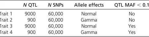
Table 3 Summary of simulated traits and number of SNPs used for analysis
NQTL NSNPs Allele effects QTL MAF,0.1
Trait 1 9000 60,000 Normal No
Trait 2 900 60,000 Gamma No
Trait 3 9000 60,000 Normal Yes
Trait 4 900 60,000 Gamma Yes
BayesC (Habieret al.2011), Bayesian Lasso [Lasso1 (Nadaf
et al.2012) and Lasso2 (de los Campos and Perez 2010)], and genomic best linear unbiased prediction (GBLUP) implemented in ASReml (Gilmouret al.2009) with a geno-mic relationship matrix as in Yanget al.(2010). All genomic prediction methods and specific implementations used are described in detail in de los Campos et al. (2012) (GS-CROSS Site /). Here we provide only information on hyperparameters and length of chains run for the various methods (Supporting Information,Table S3).
Simulation of genomes and genetic values
The simulated data sets used here are the example data from Hickey and Gorjanc (2012). Briefly, a population history of Holstein cattle was simulated. There were 1,670,000 loci seg-regating on 30 chromosomes and 60,000 sites were chosen as SNPs. While results using the 300,000-SNP array are not pre-sented, these data are available (Hickey and Gorjanc 2012). The 10 replicates of data consisted of four traits, each with different models of additive genetic variation (Table 3). The number of QTL were 9000 for trait 1, reflecting a complex trait, and 900 for trait 2. Traits 3 and 4 had the minor allele fre-quency of the QTL restricted to be ,0.1. Once a steady-state base population had been simulated, 10 more generations were created. Individuals in generations 4 and 5 were combined into a reference population of size 2000 to predict genomic breeding values for 500 individuals each in generations 6, 8, and 10 (i.e.,
N= 1500). The heritability of the traits was 0.25. Summary statistics regarding the simulated traits are given in Table 3.
The simulator of Hickey and Gorjanc (2012) attempted to combine favorable features of both coalescent and forward in time simulation approaches. While it has been recently pointed out (Woolliams and Corbin 2012) that the coales-cent is not fully suited to application in livestock populations with population histories like those simulated in these data sets (large ancient and small current effective population sizes), the data do appear to match reasonably well to the theoretical expectations of such genomic data (see below). Furthermore, the results of analysis of the data with various genomic prediction algorithms also match reasonably well with those observed in real data sets. In addition, almost identical approaches to simulating genomic data have been used in a number of studies that compare simulated and real data analysis for a number of applications, including the understanding of genomic prediction (Clark et al. 2011a, 2012) and the phasing (Hickey et al. 2011) of genotypes. The results for the analysis of simulated and real data in these and other relevant studies showed very similar trends.
However, despite the data appearing to be reasonably well behaving, it is important to recognize that there may be some theoretical weaknesses with the approach taken to simulate the data. In generating the example simulated data sets, the forward in time approach was used for the last 10 generations of the pedigree.
Pine and wheat data
The pine tree data are described in Resende et al. (2012) and contained 850 individuals with phenotypes (two traits: DBH, diameter at breast height; HT, height; age = 6 years, predicted and validated only in location Nassau) and geno-type (4698 markers) data. The following additional edits were performed on the pine data set, and missing SNPs were
filled in by sampling alleles from a Bernoulli distribution with variance equal to the locus allele frequency. Individuals and loci were removed if they contained .20% missing values. The wheat data [available through R package BLR (de los Campos and Perez 2010)] contained 599 lines with phenotype (four traits) and genotype (1279 markers) data and no further edits were performed.
Validation schemes
In the simulated data, true breeding values were generated and used for validation. In the pine and wheat data highly accurate observed values were not available and, therefore, 10-fold cross-validation was used. Both data sets were
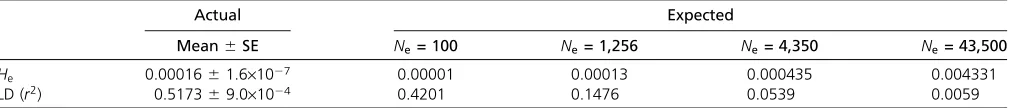
Table 4 Actual (mean and SE of 10 replicates) and expected heterozygosity,He, and linkage disequilibrium between adjacent loci,r2, in
simulated data
Actual Expected
Mean6SE Ne= 100 Ne= 1,256 Ne= 4,350 Ne= 43,500
He 0.0001661.6·1027 0.00001 0.00013 0.000435 0.004331
LD (r2) 0.517369.0·1024 0.4201 0.1476 0.0539 0.0059
Figure 1 Linkage disequilibrium (r2) at various genomic distances in
randomly assigned to one of 10 folds. Each fold was dropped once from the reference set and predicted. Accuracy (Pearson’s correlation) and regressions were calculated within each fold and the mean and SE across all folds are reported.
Indexes for reporting relationships
All relationship measures were calculated for each valida-tion individual. Mean relavalida-tionship is ð1= NPÞ
PNP
j¼1relði;jÞ, where relði;jÞ is the relationship in A or G of validation individual iand reference individualj, andNP is the num-ber of reference individuals. Mean of squared relation-ships isð1= NPÞ
PNP
j¼1relði;jÞ 2
and mean of top 10 relationships is ð1=10ÞPTop10
j¼1 relði;jÞ, where Top10 are the 10 largest relði;jÞ. In each replicate validation individuals were sorted based on these relationship measures from lowest to highest
and Pearson’s correlations were calculated between esti-mated and true breeding values in bins of 50 individuals. These empirical accuracies were then regressed onto the mean relationship measure per bin. Accuracies from the pre-diction error variance were calculated as pffiffiffiffiffiffiffiffiffiffiffiffiffiffiffiffiffiffiffiffiffiffiffiffiffiffiffi12SE2½VarðGÞ21, where SE is the standard error of prediction per individual obtained from the GBLUP analysis and Var(G) is the addi-tive genetic variance from GBLUP.
Results
Evaluation of simulated genomes
The mean minor allele frequency of the 60,000-SNP array across all simulated replicates was 0.2076 (SE = 3.0·1024). The mean heterozygosity and r2 of all replicates was
compared to expected values. The heterozygosity of the ran-domly selected markers in the 60,000-SNP set was 0.2815 (SE = 2.9·1024). Given a genome of 3 billion bp and 1.68
million segregating sites in the base population, the mean heterozygosity (He) across all sites was 0.00016 (Table 4). Calculation of the expected value was complicated by
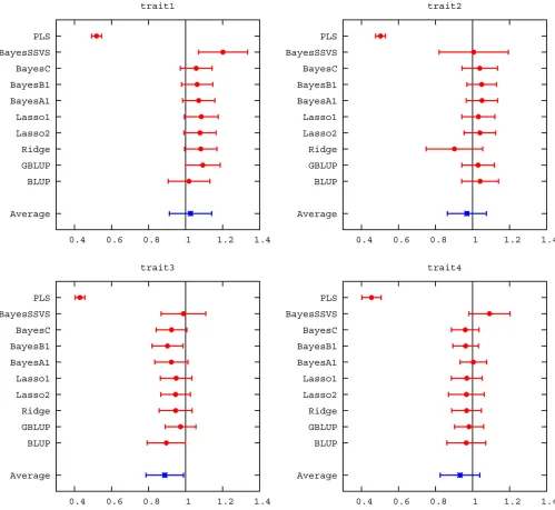
Figure 3 Regression of true breeding value on breeding values estimated with different methods (mean for validation animals in generations 6, 8, and 10).
Table 5 Mean (rel), mean squared relationships (rel2), and mean of top 10 relationships (relTop10) in matricesAandGof validation to
reference individuals in generations 6, 8 and 10 of simulated data
pBVrel
A
gBVrel
A
gBV relG
pBV rel2A
gBV rel2A
gBV rel2G
pBVrelTop10 A
gBV relTop10
A
gBV relTop10
G
Gen 6 0.0185 0.0185 20.0006 0.0013 0.0013 0.0013 0.2744 0.2744 0.2671
Gen 8 0.0185 0.0185 20.0035 0.0006 0.0006 0.0006 0.1382 0.1382 0.1216
Gen 10
0.0185 0.0185 20.0049 0.0004 0.0004 0.0004 0.0710 0.0710 0.0654
R2 0.00 0.00 0.22 0.40 0.27 0.31 0.45 0.32 0.31
R2is coefficient of determination from regressing correlations of breeding values (pedigree, pBV; and genomic, gBV) and true breeding values in bins of similarly related
changes inNeacross the simulated population history. Using
Ne = 100, the expected He was 0.00001, or an order of magnitude smaller. However, this ignores that He would have been higher in ancestral generations with greaterNe. It is expected that some ancestral alleles would still be seg-regating, thereby increasing He. The expected r2 using the formula with mutation (Tenesa et al. 2007) was 0.4201, which is lower than the pairwise r2 of 0.5173 in the simu-lations with loci ,0.05 allele frequency removed. The higher r2 may be partially explained by the N
e , 100 in the pedigree used for the last 10 generations. Figure 1 shows the drop-off inr2as distance between SNPs increases.
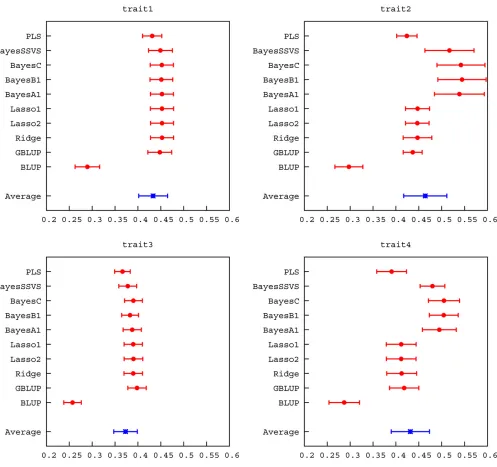
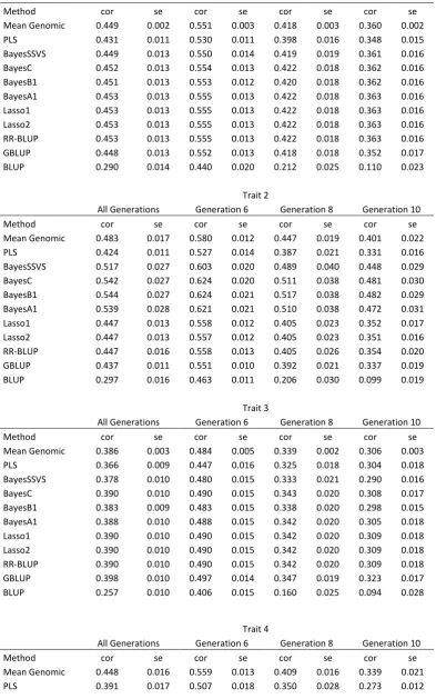
Estimates of prediction accuracy and relatedness
The genetic architectures of the example simulations were chosen so the differences between the methods were apparent. In traits 1 and 3, 9000 QTL contributed to the genetic variation whereas in traits 2 and 4 only 900 QTL were simulated. Additionally, in traits 3 and 4 the maximum minor allele frequency of the QTL was restricted to,0.1. Expectedly, most genomic methods had very similar accuracy in traits 1 and 3, once SEs were considered. In generation 6, the range of accuracy observed was 0.530– 0.554 in trait 1 and 0.447–0.497 in trait 3, as can be seen in Figure 2 and Table S1. The exception was PLS, which showed slightly lower accuracy. The trend to similar accu-racy with a high number of QTL has been observed before in several studies (e.g., Daetwyler et al. 2010b; Hayes et al.
2010; Clarket al.2011a). More diverse accuracies were pro-duced in traits 2 and 4. For these examples, variable selec-tion methods (e.g., BayesB) performed better than shrinkage methods (e.g., GBLUP, Lasso), which, in turn, outperformed PLS. The ability to either model locus-specific variances or, in addition, set some variances to zero seems to be of ad-vantage when the number of QTL is low. This has also been found in other studies (e.g., Meuwissenet al.2001; Habier
et al.2007; Lundet al.2009). The decay in accuracy across generations was very similar across methods in traits 1 and 3. However, in traits 2 and 4 shrinkage methods exhibited greater decay in accuracy as the number of generations in-creased. Accuracies using a BLUP pedigree model were in all cases lower than genomic accuracies, but were quite high in generation 6 because both parents of each individual were included in the reference population. Regressions of true on predicted breeding values varied more than accuracies, ranging between 0.429 and 1.186 across all traits in gener-ation 6. PLS, in particular, had low regression coefficients. Among the other genomic methods there was less variation. Regression coefficients of most methods were not signifi -cantly different from 1, considering their SE (Figure 3,Table S2), and regression intercepts were close to 0 for all methods.
In the simulated data, three relationship measures were calculated for both A and G, being rel, rel2, and relTop10 (Table 5). Mean rel varied little across generations and this was especially pronounced inA. A heat map ofA(replicate 1
of simulated data) is shown in Figure S1. Mean rel2 and relTop10decreased as validation individuals became further removed from the reference population. Relationships were similar inA andGbecauseGas implemented according to Yanget al.(2010) is scaled similarly toA. Consequently, the relationship between half-sibs in this version ofGis0.25. Mean relTop10 shows that individuals in generation 6 had a number of close relatives comparable to a half-sib rela-tionship level and this yielded high accuracies. The accu-racy was then calculated in bins of 50 validation individuals that were grouped according to similarity of relatedness to the reference population. The sensitivity of rel2 and relTop10
Figure 4 Regression of accuracy from prediction error variance (PEV-Ac-curacy) on mean of top 10 genomic relationships per validation individual.
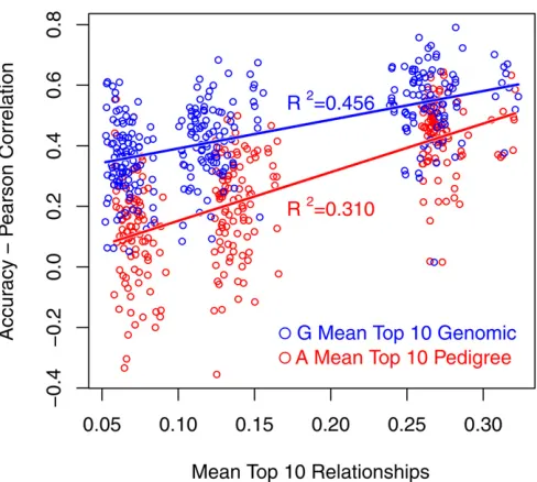
was reflected in increasedR2 when accuracy was regressed onto them (Table 5). Regression of pedigree-based accuracy exhibited a better fit to data than genomic accuracy, as expected.
As an effort to quantify the effect of relationships on the accuracy of genomic prediction, three relationship measures were calculated using both the numerator relationship matrix and the genomic relationship matrix: rel, the mean relation-ship; rel2, the mean of squared relationships; and relTop10, the mean of the top 10 relationships, where relationship refers to relationship of validation to reference individuals. Previous work has shown that rel2 and relTop10 correlated well with the accuracy from prediction error variance (PEV), while rel was less predictive (Clarket al.2012; Pszczolaet al.2012). This was confirmed in our simulated data set (Figure 4). Re-gression of accuracy from Pearson’s correlations onto these three measures had a lowerR2than when the accuracy from PEV was used in both the numerator relationship matrix (A) or the genomic relationship matrix (G) (Table 5, Figure 5). A baseline relationship of empirical accuracy and relationship measures was established using accuracy of a pure pedigree model in the regression. The R2 of this regression is higher than with genomic breeding value accuracy, but not substan-tially so. In addition, the slope of the regression using geno-mic accuracy is lower than with accuracy from pedigree prediction, as expected (Figure 5). This demonstrates that both rel2 and relTop10can provide some insight when report-ing genomic selection results.
Other relationship measures that correlate better with accuracy may exist, and which relationship measure corre-lates best with accuracy may depend on population structure.
Note that while we were able to show a relationship of relatedness and accuracy at the “macro” level (i.e., large changes in relationship across generations), we were not able to investigate this at the “micro” level (i.e., small changes in relationships within a generation) due to large sampling variances of correlations when few individuals were used in correlation bins (Figure 1). Nevertheless, Figure 5 also shows that the impact of relationships on the accuracy of genomic breeding values seems to be less than with a pedigree-based model for these examples. Further research is needed on the impact of relatedness on the ac-curacy of genomic breeding values.
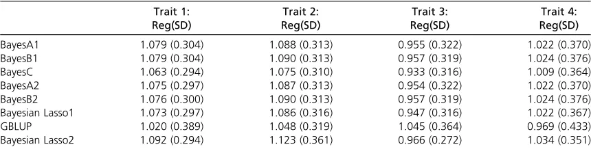
The accuracies and regressions achieved in pine and wheat with the various methods were not significantly different from each other, considering SE between folds (Tables 6, 7, and 8). The mean accuracies and regressions (in parentheses) across all methods achieved in pine DBH and HT were 0.48 (1.06) and 0.38 (1.07), respectively. Mean accuracies (and regressions) of all methods in wheat for traits 1–4 were 0.53 (1.06), 0.50 (1.07), 0.39 (0.94), and 0.46 (0.998), respectively. Intercepts of the regressions were in all the above cases close to zero (results not shown). The relationship measures rel2 and relTop10 were 0.0072 and 0.4048 for pine and 0.0086 and 0.2614 for wheat, re-spectively. Molecular markers were SNPs for pine and the genomic relationship of half-sibs using Yang et al. (2010) was 0.25. In contrast, DArT markers [only two possible genotypes (Jaccoudet al.2001)] were used in wheat, which yields an approximate half-sib genomic mean relationship of 0.125, using the Yang algorithm. It is clear therefore that the relationships between reference and validation individuals
Table 6 Accuracy of prediction and regressions for the pine data using 10-fold random cross-validation for traits diameter at breast height (DBH, age = 6 years) and height (HT, age = 6 years)
DBH: HT: DBH: HT:
Acc(SD) Acc(SD) Reg(SD) Reg(SD)
BayesA1 0.477 (0.063) 0.376 (0.108) 1.070 (0.262) 1.060 (0.398)
BayesB1 0.476 (0.066) 0.373 (0.108) 1.068 (0.266) 1.057 (0.402)
BayesC 0.478 (0.066) 0.375 (0.108) 1.061 (0.262) 1.043 (0.392)
BayesA2 0.477 (0.063) 0.376 (0.108) 1.068 (0.266) 1.059 (0.398)
BayesB2 0.475 (0.066) 0.373 (0.108) 1.068 (0.266) 1.057 (0.408)
Bayesian Lasso1 0.479 (0.066) 0.378 (0.108) 1.050 (0.259) 1.024 (0.382)
GBLUP 0.477 (0.060) 0.384 (0.095) 1.070 (0.259) 1.060 (0.351)
Bayesian Lasso2 0.481 (0.066) 0.382 (0.107) 1.105 (0.288) 1.079 (0.376)
Acc, accuracy; Reg, regression.
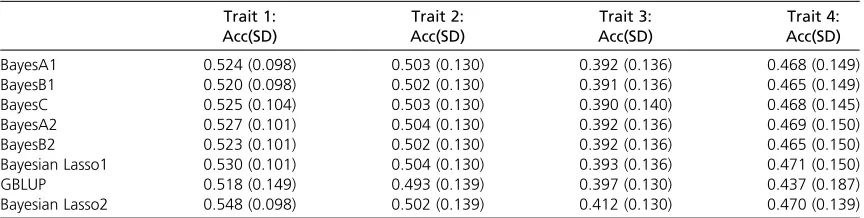
Table 7 Accuracy of prediction for the wheat data, using 10-fold random cross-validation
Trait 1: Trait 2: Trait 3: Trait 4:
Acc(SD) Acc(SD) Acc(SD) Acc(SD)
BayesA1 0.524 (0.098) 0.503 (0.130) 0.392 (0.136) 0.468 (0.149)
BayesB1 0.520 (0.098) 0.502 (0.130) 0.391 (0.136) 0.465 (0.149)
BayesC 0.525 (0.104) 0.503 (0.130) 0.390 (0.140) 0.468 (0.145)
BayesA2 0.527 (0.101) 0.504 (0.130) 0.392 (0.136) 0.469 (0.150)
BayesB2 0.523 (0.101) 0.502 (0.130) 0.392 (0.136) 0.465 (0.150)
Bayesian Lasso1 0.530 (0.101) 0.504 (0.130) 0.393 (0.136) 0.471 (0.150)
GBLUP 0.518 (0.149) 0.493 (0.139) 0.397 (0.130) 0.437 (0.187)
found in the plant data were high and this is likely the main reason for the moderately high accuracies achieved despite the quite limited number of reference individuals and markers. Lack of significant differences between method ac-curacies may have resulted from limited numbers of individ-uals and markers and the possibility of a genetic architecture of the traits where many loci contribute to the genetic var-iance and the high relationships present in the plant data sets.
Benchmarking of methods
We have investigated a few example simulated data sets and two real data sets for the most widely used genomic prediction methods. The simulated data from Hickey and Gorjanc (2012) were modeled after the population history of Holstein cattle and the real data sets were of pine and wheat (de los Campos and Perez 2010; Resende et al.
2012). This encompasses two outbreeding plant and animal populations and an inbreeding plant species, as well as dif-ferent genome ploidies. We strongly recommend further benchmarking in other populations, which may differ in population history, genome structure, and other aspects rel-evant to genomic prediction.
In the simulated data examples, traits 1 and 3 had genetic architectures where many loci affected the traits and all methods performed similarly. A slight advantage of variable selection methods was observed in traits 2 and 4, where fewer loci contributed to genetic variation. In the real data sets, all methods also achieved similar accuracy. This indicated that the traits are likely complex or that our real data sets were too small to show differences. This change in ranking depending on genetic architecture has also been observed in other studies, both in real (e.g., Hayes et al. 2009a; VanRaden
et al. 2009b) and simulated (e.g., Daetwyler et al. 2010b; Clark et al.2011a) data. Due to this dependency, no single method emerges that could serve as a benchmark for newly developed methods. We suggest that two methods, one where loci are weighted equally (e.g., GBLUP) and one where some loci are given greater emphasis (e.g., Bayes B), be used when comparing new approaches. This will ensure a rigorous com-parison of new methods to commonly used methods regard-less of trait genetic architecture. Ideally, the implementations of GBLUP and BayesB would be previously validated to avoid comparisons to suboptimal implementations, as there are
many small details related to implementation that can affect performance. However, the main point is to test new methods in varying genetic architectures to ensure that dependencies are known.
We recommend further benchmarking and testing of methods in many more real animal and plant populations as well as simulation studies with extensive replication. Our results for these examples should be confirmed with higher marker densities and, eventually, with resequencing data. It will remain important that a variety of genetic architectures are explored when benchmarking methods in dense marker data or in other variants such as small insertions and deletions. Genomic prediction has grown to be a scientific area of considerable impact in both animal and plant breeding. We have no doubt that further advances are possible to improve not only the accuracy of genomic prediction, but also the efficiency with which such predictions can be made. The utility of such advances will be evaluated with a toolkit containing results from real and simulated data, which are rigorously validated.
Acknowledgments
The authors acknowledge D. J. de Koning and Lauren McIntyre for encouraging us to write this review article and for comments provided on earlier versions of this manuscript. H.D.D. acknowledges funding from the Co-operative Research Centre for Sheep Industry Innovation. J. M.H. was funded by the Australian Research Council project LP100100880 of which Genus Plc., Aviagen Ltd., and Pfizer are co-funders. M.P.L.C. acknowledges financial support from the Dutch Ministry of Economic Affairs, Agriculture, and Innovation (Program “Kennisbasis Research”, code KB-17-003.02-006).
Note added in proof: Seede los Campos et al.2013 (pp. 327–345) for a related work.
Literature Cited
Amer, P. R., and G. Banos, 2010 Implications of avoiding overlap between training and testing data sets when evaluating genomic predictions of genetic merit. J. Dairy Sci. 93: 3320–3330. Bernardo, R., and J. Yu, 2007 Prospects for genomewide selection
for quantitative traits in maize. Crop Sci. 47: 1082–1090.
Table 8 Regression coefficients (phenotypes regressed on predicted genomic breeding values) for the wheat data, using 10-fold random cross-validation
Trait 1: Trait 2: Trait 3: Trait 4:
Reg(SD) Reg(SD) Reg(SD) Reg(SD)
BayesA1 1.079 (0.304) 1.088 (0.313) 0.955 (0.322) 1.022 (0.370)
BayesB1 1.079 (0.304) 1.090 (0.313) 0.957 (0.319) 1.024 (0.376)
BayesC 1.063 (0.294) 1.075 (0.310) 0.933 (0.316) 1.009 (0.364)
BayesA2 1.075 (0.297) 1.087 (0.313) 0.954 (0.322) 1.022 (0.370)
BayesB2 1.076 (0.300) 1.090 (0.313) 0.957 (0.319) 1.024 (0.376)
Bayesian Lasso1 1.073 (0.297) 1.086 (0.316) 0.947 (0.316) 1.022 (0.367)
GBLUP 1.020 (0.389) 1.048 (0.319) 1.045 (0.364) 0.969 (0.433)
Bijma, P., 2012 Accuracies of estimated breeding values from or-dinary genetic evaluations do not reflect the correlation between true and estimated breeding values in selected populations. J. Anim. Breed. Genet. 129: 345–358.
Calus, M., and R. Veerkamp, 2011 Accuracy of multi-trait genomic selection using different methods. Genet. Sel. Evol. 43: 26. Calus, M. P. L., 2010 Genomic breeding value prediction: methods
and procedures. Animal 4: 157–164.
Calus, M. P. L., T. H. E. Meuwissen, A. P. W. de Roos, and R. F. Veerkamp, 2008 Accuracy of genomic selection using different methods to define haplotypes. Genetics 178: 553–561. Chen, G. K., P. Marjoram, and J. D. Wall, 2009 Fast andflexible
simulation of DNA sequence data. Genome Res. 19: 136–142. Clark, S., J. Hickey, and J. van der Werf, 2011a Different models
of genetic variation and their effect on genomic evaluation. Genet. Sel. Evol. 43: 18.
Clark, S., J. M. Hickey, and J. H. J. van der Werf, 2011b Proceedings of the Association for the Advancement of Animal Breeding and Genetics. 19–21 July 2012, edited by P. Vercoe. Association for the Advancement of Animal Breeding and Genetics, Perth, Australia, Vol. 19, pp. 291–294.
Clark, S. A., J. M. Hickey, H. D. Daetwyler, and J. H. J. Van der Werf, 2012 The importance of information on relatives for the prediction of genomic breeding values and implications for the makeup of reference populations in livestock breeding schemes. Genet. Sel. Evol. 44: 4.
Cleveland, M. A., J. M. Hickey, and S. Forni, 2012 A common data-set for genomic analysis of livestock populations. G3 2: 429–435. Coster, A., and J. Bastiaansen, 2009 HaploSim: R-package version 1.8-4. http://cran.r-project.org/web/packages/HaploSim/index. html.
Crossa, J., G. l. Campos, P. Perez, D. Gianola, J. Burgueno et al., 2010 Prediction of genetic values of quantitative traits in plant breeding using pedigree and molecular markers. Genetics 186: 713–724.
Daetwyler, H. D., 2009 Genome-wide evaluation of popula-tions. Ph.D. Thesis, Wageningen University, Wageningen, The Netherlands.
Daetwyler, H. D., B. Villanueva, P. Bijma, and J. A. Woolliams, 2007 Inbreeding in genome-wide selection. J. Anim. Breed. Genet. 124: 369–376.
Daetwyler, H. D., B. Villanueva, and J. A. Woolliams, 2008 Accuracy of predicting the genetic risk of disease using a genome-wide approach. PLoS ONE 3: e3395.
Daetwyler, H. D., J. M. Hickey, J. M. Henshall, S. Dominik, B. Gredleret al., 2010a Accuracy of estimated genomic breeding values for wool and meat traits in a multi-breed sheep popula-tion. Anim. Prod. Sci. 50: 1004–1010.
Daetwyler, H. D., R. Pong-Wong, B. Villanueva, and J. A. Woolliams, 2010b The impact of genetic architecture on genome-wide evaluation methods. Genetics 185: 1021–1031.
Daetwyler, H. D., K. E. Kemper, J. H. J. van der Werf, and B. J. Hayes, 2012 Components of the accuracy of genomic prediction in a multi-breed sheep population. J. Anim. Sci. 90: 3375–3384. Dekkers, J. C. M., and F. Hospital, 2002 The use of molecular
genetics in the improvement of agricultural populations. Nat. Rev. Genet. 3: 22–32.
de los Campos, G., and P. Perez, 2010 BLR: Bayesian linear re-gression. R-package version 1.2.http://cran.r-project.org/web/ packages/BLR/index.html.
de los Campos, G., J. M. Hickey, R. Pong-Wong, H. D. Daetwyler, and M. P. L. Calus, 2013 Whole genome regression and prediction methods applied to plant and animal breeding. Genetics 193: 327–345.
De Roos, A. P. W., B. J. Hayes, and M. E. Goddard, 2009 Reliability of genomic breeding values across multiple populations. Genetics 183: 1545–1553.
Donnelly, P., and T. G. Kurtz, 1999 Genealogical processes for Fleming-Viot models with selection and recombination. Ann. Appl. Probab. 9: 1091–1148.
Efron, B., and G. Gong, 1983 A leisurely look at the bootstrap, the jackknife, and cross-validation. Am. Stat. 37: 36–48.
Erbe, M., E. C. G. Pimentel, A. R. Sharifi, and H. Simianer, 2010 Assessment of cross-validation strategies for genomic prediction in cattle, pp. 129–132 in 9th World Congress of Genetics Applied to Livestock Production, edited by German Society for Animal Science. German Society for Animal Science, Leipzig, Germany.
Falconer, D. S., and T. F. C. Mackay, 1996 Introduction to Quan-titative Genetics. Longman, Harlow, UK.
Fearnhead, P., 2003 Ancestral processes for non-neutral models of complex diseases. Theor. Popul. Biol. 63: 115–130.
Fisher, R. A., 1915 Frequency distribution of the values of the correlation coefficient in samples from an indefinitely large pop-ulation. Biometrika 10: 507–521.
Gilmour, A. R., B. Gogel, B. R. Cullis, and R. Thompson, 2009 2009 ASReml User Guide Release 3.0. VSN International, Hemel Hempstead, UK.
Goddard, M. E., 2009 Genomic selection: prediction of accuracy and maximisation of long term response. Genetica 136: 245–252. Goddard, M. E., and B. J. Hayes, 2009 Mapping genes for complex traits in domestic animals and their use in breeding programmes. Nat. Rev. Genet. 10: 381–391.
Groenen, M., H.-J. Megens, Y. Zare, W. Warren, L. Hillieret al., 2011 The development and characterization of a 60K SNP chip for chicken. BMC Genomics 12: 274.
Habier, D., R. L. Fernando, and J. C. M. Dekkers, 2007 The impact of genetic relationship information on genome-assisted breeding values. Genetics 177: 2389–2397.
Habier, D., J. Tetens, F.-R. Seefried, P. Lichtner, and G. Thaller, 2010 The impact of genetic relationship information on genomic breeding values in German Holstein cattle. Genet. Sel. Evol. 42: 5. Habier, D., R. Fernando, K. Kizilkaya, and D. Garrick, 2011 Extension of the Bayesian alphabet for genomic selection. BMC Bioinfor-matics 12: 186.
Hastie, T., R. Tibshirani, and J. Friedman, 2001 The Elements of Sta-tistical Learning. Springer Science and Business Media, New York. Hayes, B. J., P. J. Bowman, A. J. Chamberlain, and M. E. Goddard,
2009a Invited review: genomic selection in dairy cattle: prog-ress and challenges. J. Dairy Sci. 92: 433–443.
Hayes, B. J., P. J. Bowman, A. J. Chamberlain, K. L. Verbyla, and M. E. Goddard, 2009b Accuracy of genomic breeding values in multi-breed dairy cattle populations. Genet. Sel. Evol. 41: 51. Hayes, B. J., H. D. Daetwyler, P. J. Bowman, G. Moser, B. Tieret al.,
2009c Accuracy of genomic selection: comparing theory and results, pp. 352–355 in Proceedings of the Association for the Advancement of Animal Breeding and Genetics, Barossa Valley, Australia, Vol. 18, pp. 352–355.
Hayes, B. J., P. M. Visscher, and M. E. Goddard, 2009d Increased accuracy of artificial selection by using the realized relationship matrix. Genet. Res. 91: 47–60.
Hayes, B. J., J. Pryce, A. J. Chamberlain, P. J. Bowman, and M. E. Goddard, 2010 Genetic architecture of complex traits and ac-curacy of genomic prediction: coat colour, milk-fat percentage, and type in Holstein cattle as contrasting model traits. PLoS Genet. 6: e1001139.
Heffner, E. L., M. E. Sorrels, and J.-L. Yannink, 2009 Genomic selection for crop improvement. Crop Sci. 49: 1–12.
Henderson, C. R., 1984 Applications of linear model in animal breeding. University of Guelph, Guelph, ON, Canada.