Cancer-COVID-19 Mortality Prediction:- An
Algorithm by Bayesian Autoregressive Model
Atanu Bhattacharjee
Section of Biostatistics,Centre for Cancer Epidemiology,
Tata Memorial Centre, Mumbai,India
Hombi Bhaba National Institute,Mumbai,India
April 23, 2020
Abstract
This pandemic of COVID-19 is tedious to control. The only lockdown is the way to stop the spread of this infection. Conventional health care is fac-ing a real challenge to operate. Primarily the challenge is to provide health care support for COVID-19 patients with limited resources and continue the health care services like earlier.Perhaps, this challenge is the same but mag-nitude is different from different geographical locations around the globe. In this article, we presented a Bayesian algorithm with the Code to predict can-cer death due to COVID-19. This code is possible to run at different time points and different geographical locations around the world. This code will help us to get the best strategy and shift the treatment option for cancer treatment. The model would provide physicians with an objective tool for counseling and decision making at different hotspots and small areas to im-plement.
Keywords:-COVID-19; Cancer; Decision; Bayesian, autoregressive model;
Introduction
In this current COVID-19 pandemic, we are waking up to the limitations of their analog health care system. We need an immediate digital solution,
pursued on several fronts, to address this crisis. It is crucial to implement predicting maps during this outbreak and attain all possible ways to explore an estimation of transmission rate who infected whom, where, when and what the rate? But it is difficult to understand the transmission because it is not known always.We can find out when a particular host individual contacted the infection, and thereafter transmitted to others. It is required to uncover the transmission process case to cases to create dynamic models.
Lockdown is the only solution to stop the COVID-19 pandemic. We do not have sufficient data with cancer and COVID-19. Are cancer patients prone to get infected? Do they have more complications? The consequence of infection is death. What is the risk of death due to COVID-19 among can-cer patients? Broadly, any active treatment is a management of cancan-cer by prolonging death occurrence. Similarly, lockdown is to halt the infection and deaths. Now the concern is about to halt the treatment for cancer or continue it? We preferred to perform the Bayesian autoregressive modeling. A total of 28 days of India’s COVID-19 confirmed and mortality data is considered. The autoregressive model is used to predict the next 50 days’ projections on mortality and confirmed cases for the general population and cancer pa-tients.The simulated data has generated the predict the cancer COVID-19 death for illustration.
The univariate Bayesian approach is an already established method. It is possible to obtain parameter estimation by iterative generalized least square [6, 7]. The most common approach is the generalize the conditional au-toregressive (CAR) distribution [1].The multivariate approach is already ex-plored [2–5].Ths autoregressive approach is valid to predict the COVID-19 disease. We apply the autoregressive model in the COVID-19 India model.
to implement.The model is easy to run in OpenBUG software to generate the prediction. The OpenBUG software is opensource. It is possible to generate prediction with convergence with updated real time data.
Statistical Model
Linear Autoregressive Regression
A linear model is defined as
Y(t) =β0+β1X1(t) +β2X2(t) =...+βmXm(t) +Z(t) (1)
It is defined as Y(t) as the observation of the dependent variable at time t. Now Xi(t) is presented as the i-th independent variable at time t, and finally Z(t) is the error term at timet. The errorsZ(t);t= 1,2...., nterm is assumed with mean zero ,have a constant variance, and autocorrelated. Now objective is to compute the Bayesain inference for the m with regression coefficientβi.
The unknown parameters of the error process. It is assumed that Z(t) to follow AR(1) with autocorrelation θ.
Non-linear Autoregressive Model
However, the number of cases count is unknown in the future. It may progress by non-linear trends. The non-linear autoregressive modeling is defined as
Y(t) = exp(β0+β1t) +Z(t) (2)
Similarly, the intercept is presented as β0 and the regression parameter isβ1
are not known. The corresponding error for this model is estimated at Z(t). The autocorrelation θ with AR(1) process is assumed. The OpenBUG code is presented below. Suppose the observations is assumed as t. The Bayesian computation is performed with 28 observations i.e. 4 weeks count data. It helped to estimates ofβ0, β1 andθ,andσ2respectively. A total of 30,000
Result
Indian confirmed, recovered and death count data are presented (Figure1) for the last 28 days. It shows the real and overwhelming success of lockdown to retains the case count with limited numbers. Perhaps, death is contributed to a marginal proportion. The available data on https://www.mohfw.gov.in/ website is presented. It presents a comparison between the proportion of death and recovery among confirmed cases (Figure 2 (A)). Similarly, a 10% higher rate of death among cancer patients with similar recovery rates is presented (Figure 2(B)). Further, we applied the Bayesian auto-regressive model. The autoregressive model is separated into linear and non-linear models. The linear model is defined in equation(1). Similarly, the non-linear model is presented in equation (2).
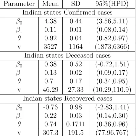
The posterior estimates of the regression coefficients are obtained by the linear autoregressive model. The model is performed for confirmed, recov-ered and died cases separately. The result of posterior estimates is presented in Table 1. A total of four parameters are estimated. The β0 and β1
repre-sents the intercept and regression coefficients. The variance of the model is presented by v. the amount of autocorrelation is estimated by θ. A total of 30,000 iterations are performed to obtain convergence and estimates. Now the linear autoregressive model is defined as Model 1( for confirmed cases), Model 2( for died case) and Model 3( recovered cases). The linear model simulation is presented in Figure 4. It shows to obtain the converges for the parameters. The posterior estimates of the non-linear model are presented in Table 2. The posterior regression estimates of all the parameters can be used for prediction of the case and death count for the next 50 days (figure 3).The OpenBUG code is presented below can be used to obtain the predic-tion. It shows that the death count among cancer patients is relatively high. The treatment provision with lockdown may challenge cancer death. Can-cer patients may die due to COVID-19 infection and simultaneously without treatment due to cancer.
Conclusion
basis about providing the treatment and reduce mortality due to cancer. Because the attempt to reduce mortality due to cancer can incline death due to COIVD-19 and spread of infection. The spread of infection will also put other non-cancer individuals into a risk. We hope to help head and neck cancer patients to survive this crucial period.
Acknowledgement
None.
Conflict of interest
No
Table 1: Linear Autoregressive Posterior Estimates of Confirmed, deceased and recovered cases on prediction.
Parameter Mean SD 95%(HPD) Indian states Confirmed cases
β0 4.38 0.44 (3.56,5.11)
β1 0.11 0.01 (0.08,0.14)
θ 0.92 0.04 (0.82,0.97)
v 3527 1164 (1873,6366)
Indian states Deceased cases
β0 0.38 0.52 (-0.72,1.51)
β1 0.13 0.02 (0.09,0.17)
θ 0.71 0.17 (0.34,0.95)
v 46.29 27.33 (10.29,110.9 Indian states Recovered cases
β0 -0.76 0.98 (-0.71,1.41)
β1 0.22 0.03 (0.14,0.30)
θ 0.74 0.17 (0.36,.96)
Table 2: Non-linear Autoregressive Posterior Estimates of Confirmed, de-ceased and recovered cases on prediction.
Parameter Mean SD 95%(HPD)
Indian states Confirmed cases
β0 4.38 0.44 (3.56,5.11)
β1 0.11 0.01 (0.08,0.14)
θ 0.92 0.04 (0.82,0.97)
v 3527 1164 (1873,6366)
Indian states Deceased cases
β0 0.38 0.52 (-0.72,1.51)
β1 0.13 0.02 (0.09,0.17)
θ 0.71 0.17 (0.34,0.95)
v 46.29 27.33 (10.29,110.9) Indian states Recovered cases
β0 -0.76 0.98 (-2.83,1.41)
β1 0.22 0.03 (0.14,0.30)
θ 0.74 0.1711 (0.36,0.96) v 307.3 191.5 (77.96,767)
OpenBUGS Model
model
{
beta0 ∼ dnorm(0,.001) beta1∼ dnorm(0,.001) theta∼dbeta(6,4) v∼ dgamma(.001,.001)
for( t in 1:28){mu[t]<-exp(beta0+beta1*t) Y[1,1:28]∼ dmnorm(mu[],tau[,])
tau[1:28,1:28]<-inverse(Sigma[,])
for(i in 1:28){Sigma[i,i]<-v/(1-theta*theta)
for(i in 1:28){for(j in i+1:28)Sigma[i,j]<- v*pow(theta,j)*1/ (1-theta*theta)}}
for( i in 2:28) for(j in 1: i-1)Sigma[i,j]<-v*pow(theta,i-1)*1/ (1-theta*theta)}}
Indian states Confirmed cases list(
Figure 1: The comparison between the official COVID-19 pandemic data of confirmed, died and recovered. cases in India.
Prediction of Confirmed cases from posterior regression estimates
set.seed(1)
w<-rnorm(100,sd =59.38) z<-rep(0,100)
for ( t in 2:100) z[t]<-0.92*z[t-1]+w[t] Time<-1:100
f<- function(x) exp(4.38+0.11*x) x<-f(Time)+z
Figure 2: The comparison between died and recovered proportion in general population(A) and cancer patients(B).
References
[1] Julian Besag. Spatial interaction and the statistical analysis of lattice sys-tems. Journal of the Royal Statistical Society: Series B (Methodological), 36(2):192–225, 1974.
Figure 3: The prediction of case count and death count for next 50 days in general population and cancer patients.
[3] W Keith Hastings. Monte carlo sampling methods using markov chains and their applications. 1970.
[4] Xiaoping Jin, Sudipto Banerjee, and Bradley P Carlin. Order-free co-regionalized areal data models with application to multiple-disease map-ping. Journal of the Royal Statistical Society: Series B (Statistical Methodology), 69(5):817–838, 2007.
[5] Hoon Kim, Dongchu Sun, and Robert K Tsutakawa. A bivariate bayes method for improving the estimates of mortality rates with a twofold conditional autoregressive model. Journal of the American Statistical association, 96(456):1506–1521, 2001.
Figure 4: Iteration convergence of different parameters.
of the Royal Statistical Society: Series C (Applied Statistics), 48(2):253– 268, 1999.