Concurrent Secure Computation with Optimal Query Complexity

Concurrent Secure Computation with

Optimal Query Complexity

Ran Canetti ∗ Vipul Goyal† Abhishek Jain‡

Abstract

The multiple ideal query (MIQ) model [Goyal, Jain, and Ostrovsky, Crypto’10] offers a relaxed notion of security for concurrent secure computation, where the simulator is allowed to query the ideal functionalitymultiple times per session(as opposed to just once in the standard definition). The model provides a quantitative measure for the degradation in security under concurrent self-composition, where the degradation is measured by the number of ideal queries. However, to date, all known MIQ-secure protocols guarantee only an overall average bound on the number of queries per session throughout the execution, thus allowing the adversary to potentially fully compromise some sessions of its choice. Furthermore, [Goyal and Jain, Eurocrypt’13] rule out protocols where the simulator makes only an adversary-independent constant number of ideal queries per session.

We show the first MIQ-secure protocol with worst-case per-session guarantee. Specifically, we show a protocol for any functionality that matches the [GJ13] bound: The simulator makes only aconstantnumber of ideal queries ineverysession. The constant depends on the adversary but is independent of the security parameter.

An immediate corollary of our main result is in extending the password authenticated key exchange (PAKE) protocol of [GJO10] from the case of a single password to the general case of multiple arbitrary passwords. Specifically, we give the first PAKE protocol for the fully concurrent, multiple password setting in the standard model with no set-up assumptions.

1

Introduction

General feasibility results for secure computation were established nearly three decades ago in the seminal works of [Yao86,GMW87]. However, these results only promise security for a protocol if it is executed in isolation, “unplugged” from any network activity. In particular, these results are not suitable for the Internet setting where multiple protocol executions may occur concurrentlyunder the control of a common adversary.

A brief history of concurrent security. Towards that end, an ambitious effort to understand and design concurrently secure protocols kicked into gear with early works such as [GK96,DDN00a],

∗

Boston University and Tel Aviv University. Email: [email protected]. Supported by the Check Point Institute for Information Security, ISF grant 1523/14, and NSF Frontier CNS 1413920 and 1218461 grants.

†

Microsoft Research India. Email: [email protected] ‡

and later the study of the concurrent zero knowledge setting [DNS98, RK99, CKPR01, KP01,

PRS02]. For other functionalities and in more general settings, however, far-reaching impossibility results were established [CF01,CKL03, Lin03,BPS06,Goy12,AGJ+12, GKOV12]. These results refer to the “plain model” where the participating parties have no trusted set-up, and hold even if the parties have access to pairwise authenticated communication and a broadcast channel.

Two main lines of research have emerged in order to circumvent these impossibility results. The first concerns with the use of trusted setup assumptions such as a common random string, strong public key infrastructure or tamper-proof hardware tokens (see, e.g. [CLOS02,BCNP04,Kat07]). The second line of research is dedicated to the study of weaker security definitions that allow for positive results in the plain model, without additional trust assumptions. The most notable examples of this include security w.r.t. super-polynomial time simulation [Pas03, PS04, BS05,

CLP10,GGJS12] and input-indistinguishable computation [MPR06,GGJS12]. One main drawback in this line of research is that it is not always clear by “how much” is the definition of security relaxed, or in other words “how much security” is being lost due to concurrent attacks.

The multiple ideal query model and its applications. The multiple ideal query model (or, the MIQ model in short) of Goyal, Jain and Ostrovsky [GJO10] takes a different approach to the problem of quantifying the security loss. In this model, the simulator is allowed to query the ideal functionality multiple times per session (as opposed to just once in the standard definition). On the technical side, allowing the simulator multiple queries indeed facilitates proofs of security in a concurrent setting. On the conceptual side, this model allows for a natural quantification of the “security loss” incurred by concurrent attack: the more ideal queries, the weaker the security guarantee. Furthermore, the effect of multiple ideal queries strongly depends on the task at hand, thus allowing for more fine-tuned notions of security for a given problem or setting.

One functionality where this approach proved very effective is that of password-based key ex-change (namely the two-party function that outputs a secret random value to both parties if the inputs provided by the two parties are equal). When the number of queries made by the simulator per session is a constant, the security guarantees of the MIQ model actually imply fully concurrent password-based authenticated key exchange (see [GL01,GL06,GJO10]). This fact was exploited by Goyal et. al [GJO10] to get the first concurrent PAKE in the plain model — albeit with the significant restriction that the samepassword is to be used as input in every session. This restric-tion results from a weakness in their modeling and analysis - a weakness that we overcome in this work.

Now, observe that if we only allow, say, 2 queries to a malicious P2 in the ideal world (per real world session), then as long asQ is a high-degree polynomial, the security guarantee forP1 is still quite meaningful. Instead of a single point, now a malicious adversary may learn the output on two points of its choice (from an exponential domain of points). However, the adversary still does not learn any information about what the polynomial evaluates to on rest of the domain. On the other hand, if we allow too many queries (exceeding the degree of the polynomial), then the ideal world adversary may be able to learn the entire polynomialQ!

Another related example is 1-out-of-mOT. Here, as long asλ, the simulator’s query complexity, is smaller than m, MIQ provides meaningful security which degrades gracefully with λ. More generally, the remaining security for any session iin concurrently secure computation of function f is proportional to the “level of unlearnability” off(·, xi) after q queries, where xi is the secret input of the honest party in session i. Password-based key exchange is an extreme case of an unlearnable function. Ideally, we would like to bringλas close as possible to 1.

Prior work: Average case vs. worst case guarantees. The best positive result in the MIQ model is due to Goyal, Gupta, and Jain [GGJ13] (improving upon [GJO10]). They provide a con-struction where the number of ideal queries in a session are (1 + log_n6n), where n is the security parameter. However, this is only an average-case guarantee over the sessions that provides very weak security. In particular, it does not preclude the ideal adversary from making an arbitrarily large number of queries in some chosen sessions (while keeping the number of queries low in the other sessions). In cases of interest, such as the PAKE functionality or the above oblivious poly-nomial evaluation functionality, this means that the security in some sessions may be completely compromised!

Furthermore, Goyal and Jain [GJ13] recently proved an unconditional lower bound on the num-ber of ideal queries per session. Specifically, they show that there exists a two-party functionality that cannot be securely realized in the MIQ model with any (adversary independent) constant number of ideal queries per session. A natural and important question is thus what is the best worst-case bound we can give on the number of ideal queries asked per session?

1.1 Our Results

In this work, we fully settle the question of worst-case number of per session ideal queries in the context of general function evaluation. Our main result is stated below.

Theorem 1 (Main result (informally stated)). Under standard cryptographic assumptions, for every PPT functionality f, there exists a protocol in the MIQ model where the simulator makes only a constant number of ideal queries in every session. The aforementioned constant is dependent upon the adversary, and, in particular on the number of sessions (rather than being universal).

If the number of concurrent sessions being executed by the adversary is nc, then the constant in the above theorem will be derived from c. A more detailed discussion on this can be found at the end of this subsection.

Our upper bound tightly matches the lower bound of Goyal and Jain [GJ13] which rule out protocols where the simulator makes a constant number of ideal queries per session for any universal constant. Taken together, this fully resolves the central problem in the study of the MIQ problem: a (adversary dependent) constant number of ideal queries per session is both necessary and sufficient for simulation. Thus, our work can be viewed as thefinal stepin understanding the simulator query complexity of the MIQ model.

Fully concurrent PAKE without setup. Say that a password-based key exchange protocol is fully concurrentif it remains secure in a setting where unboundedly many executions of the protocol run concurrently, on potentially different passwords. An immediately corollary of our main result is the resolution of the long standing open problem of designing a fully concurrent PAKE protocol in the standard model and with no setup assumptions:

Theorem 2 (Concurrent PAKE (informally stated)). Under standard cryptographic assumptions, there exists a fully concurrent Password-based Key Exchange protocol in the standard model and with no trusted set-up. The security of the exchanged keys is c/|D|, where D is the password dictionary and c is an adversary-dependent constant.

A discussion on adversary dependent constants. In the above theorems, if the number of concurrent sessions being executed by the adversary is nc, then the number of ideal world queries made by the simulator (in Theorem 1) or the distinguishing probabilty for the exchanged keys (in Theorem 2) is a function of c alone. We call this as an adversary dependent constant. Consider any adversary which runs in polynomial time. For such an adversary, there must exist a constant csuch that nc bounds its running time (and hence the number of concurrent sessions). Then if the number of ideal queries is a function of calone, it doesnotgrow withn. Thus overall, the number of ideal queries is a fixed constant for every polynomial time adversary (although this constant could be different for different polynomial time adversaries).

We remark that this is reminiscent of how we define and treat the running time of simulator in zero-knowledge (and other cryptographic protocols). The running time of the simulator may depend upon the running time of the adversary (and in particular upon the number of sessions in the concurrent setting), and, hence is not an a priori fixed polynomial. However for every adversary, there is a (possibly different) polynomial in the security parameter which describes the running time of the simulator.

1.2 Technical Overview

As observed in [GJO10], the study of simulator query complexity in the MIQ model can also be cast as a precise simulation problem by viewing the trusted party queries as the resource of the simulator. Therefore, advances in precise simulation strategies go hand in hand with improvements in the simulator query complexity in the MIQ model. Indeed, prior works in the MIQ model [GJO10, GGJ13] have relied upon sophisticated precise simulation strategies in order to obtain their positive results. We note, however, that till date, all precise simulation strategies only focus on minimizing thetotal costof the simulator across all the sessions. Indeed, this is why these works only yield anaverage-case bound on the simulator query complexity.

In this work, we are interested in minimizing the worst-case simulator query complexity per session. In other words, we are interested in simulation strategies that guarantee local precision for every session.

Our approach in a nutshell. Towards that end, our starting observation is that the problem of bounding the simulator query complexity per session can be reduced to bounding the number of times the output message of a session appears in the entire simulation transcript.1 In other words, we need a precise (concurrent) simulation strategy where the output message of every session appears only a constant number of times across theentire simulation transcript.2 For this purpose, we revisit existing precise simulation strategies. Concretely, we show that a slight variant of the “sparse” rewinding strategy of Goyal, Gupta and Jain [GGJ13] (that we henceforth refer to as the GGJ simulation strategy) satisfies our desired property. We prove this by a novel, purely combinatorial analysis. Our final secure computation protocol remains essentially identical to those in the prior works in the MIQ model.

We now give an overview of the steps involved in our proof. Say that we wish to analyze the number of queries in session i. Consider the specific point in the protocol execution of session i where, the simulator actually makes a query to the ideal functionality: call this point pi (for example, this may be the 5th message of the protocol execution in session i). This means that whenever the simulator reaches the point pi (in the overall concurrent execution), it will have to call the trusted functionality for session i to compute the next outgoing message. Thus, now the problem reduces to simply counting how many times the point pi occurs in the entire rewinding schedule. Observe that in each thread of execution, point pi only occurs once. However, there could be multiple threads of execution resulting because of rewinding. Therefore,pi may also occur multiple times in the rewinding schedule.

While a direct (full) analysis of the GGJ rewinding strategy [GGJ13] turns out to be complex, we are able to break it down into three different steps. Each step builds upon the previous one, with the final step yielding us the desired bound on the simulator query complexity. Below, we provide an informal overview of each of the three steps and refer the reader to the later sections for details.

Step 1. Lazy-KP withstaticscheduling: We first consider the warm-up case when scheduling of messages by the adversary is static. This means that the ordering of the messages of different sessions is decided by the adversary ahead of time and is fixed (and does not change upon rewinding

1

More concretely, we wish to bound the first message in the protocol where the simulator is forced to query the trusted party in order to obtain the function output.

2

by the simulator). Further, instead of directly analyzing the GGJ simulator [GGJ13], here we will analyze the query complexity of the (simpler) “lazy-KP” simulator [PTV14,PRS02,KP01] for the case where the simulator uses a splitting factor ofnfor rewinding. That is, during simulation, each thread is divided into nequal parts, and, each resulting part is rewound individually (resulting in different threads of execution).

In this case, we are able to prove that the simulator makes at most O(1) queries to the ideal functionality in any given session. This is done by relying on the following fact. Say that the point pi does not occur in a given thread. Then, since the adversary only employs static scheduling, this would mean that the point pi also cannot occur in any threads resulting from rewinding this thread. Thus, the proof reduces to a counting argument on the number of threads resulting from rewinding the part of the main thread containingpi. Ifdis the depth of recursion for our recursive rewinding schedule, then we are able to show that there are at mostO(2d) threads containing point pi. However, the depth dwill be a constant for lazy-KP simulation with splitting factor n.

Step 2. Lazy-KP with dynamic scheduling: Now we analyze a general adversary that may dynamically change the ordering of the messages across different sessions upon being rewound. Hence, different threads of execution may have different ordering of the messages. We shall continue to analyze the lazy-KP simulation strategy with splitting factorn.

In this case, we are able to prove that the simulator makes at most O(log(n)) queries to the ideal functionality in any given session. The key difficulty in this case is that even if a given thread does notcontain the point pi, the threads resulting from its rewinding may still have pi. Hence, it seems hard to rule out the possibility thatpi may show up in a large number of threads throughout the simulation.

To overcome this problem, we rely on the following fact: once the point pi is seen in the main thread of execution, it cannot occur in any thread arising out of the main threadafter that point. We also observe thatbefore this point is seen in the main thread, there seems hope to rule out its occurrence in a “large” number of look ahead threads. This relies on the symmetry of the main and the look-ahead threads, and, on the fact that this point has roughly equal probability of occurring first in the main thread vs occurring first in any given look ahead thread. Indeed, this step of the proof is much more involved than the first step and we refer the reader to Section 4 for more details.

Step 3. Sparsifyingthe lazy-KP simulation: In the final step, we analyze thesparse rewind-ing strategy of [GGJ13]. Very roughly speaking, the sparse rewinding strategy of [GGJ13] aims to rewind the adversary in “as few places as possible” while still solving all the sessions. More specifically, there is a cost associated with creating each look ahead, and, the goal of the rewinding strategy is to solve all sessions while minimizing the cost.

The key idea of our final step is to leverage this sparsification in order the reduce the number of queries from O(log(n)) from the previous step to O(1). Recall from above that if we were to use the full lazy-KP simulation, the pointpi would have occurred atO(log(n)) places in the entire simulation. However, now, in the GGJ rewinding strategy, it will occur only O(1) times because most of the threads will never be executed. More details are given in section5.

2

Our Model

We define our security model by extending the standard real/ideal paradigm for secure computation. Roughly speaking, we consider a relaxed notion of concurrently secure computation where the ideal world adversary is allowed to make an a priori fixed λ number of output queries to the ideal functionality for each session. Note that in contrast, the standard definition for concurrently secure computation only allows foroneoutput query per session to the ideal adversary. We now give more details.

Notation. Letndenote the security parameter. We denote computational indistinguishability by c

≡. In this work, we consider malicious, static adversaries that choose whom to corrupt before the start of any protocol. Further, we work in the static input setting, i.e., we assume that the inputs of the honest parties in all sessions are fixed at the beginning. We do not require fairness.

Ideal model. We first define the ideal world experiment, where there is a trusted party for computing the desired two-party functionality f. Let there be two parties P1 and P2 that are involved in multiple, saym=m(n), evaluations off.3 LetSdenote the adversary. The ideal world execution (parameterized by λ) proceeds as follows.

I. Inputs: P1 and P2 obtain a vector of m inputs, denoted ~x and ~y respectively. The adversary is given auxiliary input z, and chooses a party to corrupt. Without loss of generality, we assume that the adversary corruptsP2 (when the adversary controlsP1, the roles are simply reversed). The adversary receives the input vector~y of the corrupted party.

II. Session initiation: The adversary initiates a new session by sending a start-session message to the trusted party. The trusted party then sends (start-session, i) toP1, whereiis the index of the session.

III. Honest parties send inputs to trusted party: Upon receiving (start-session, i) from the trusted party, honest party P1 sends (i, xi) to the trusted party, where xi denotesP1’s input for session i.

IV. Adversary sends input to trusted party and receives output: Whenever the adversary wishes, it may send a message (i, `, y<sub>i,`</sub>0 ) to the trusted party for any y<sub>i,`</sub>0 of its choice. Upon sending this pair, it receives back (i, `, f(xi, y0_i,`)) where xi is the input value that P1 previ-ously sent to the trusted party for sessioni. The only limitation is that for anyi, the trusted party accepts at mostλtuples indexed by ifrom the adversary.

V. Adversary instructs trusted party to answer honest party: When the adversary sends a message of the type (output, i, `) to the trusted party, the trusted party sends (i, f(xi, y<sub>i,`</sub>0 )) toP1, wherexi and y0_i,` denote the respective inputs sent by P1 and adversary for sessioni. 3

VI. Outputs: The honest party P1 always outputs the values f(xi, yi,`0 ) that it obtained from the trusted party. The adversary may output an arbitrary (probabilistic polynomial-time computable) function of its auxiliary inputz, input vector~y and the outputs obtained from the trusted party.

The ideal execution of a function F with security parameter n, input vectors ~x, ~y and auxiliary input z toS, denoted IdealF,S(n, ~x, ~y, z), is defined as the output pair of the honest party and S from the above ideal execution.

Definition 1 (λ-Ideal Query Simulator). Let S be a non-uniform probabilistic (expected) ppt

machine representing the ideal-model adversary. We say that S is a λ-ideal query simulator if it makes at most λoutput queries per session in the above ideal experiment.

Real model. Let Π be a two-party protocol for computing F. Let A denote a non-uniform probabilistic polynomial-time adversary that controls eitherP1 orP2. The parties run concurrent executions of the protocol Π, where the honest party follows the instructions of Π in all executions. The honest party initiates a new sessioniwith inputxiwhenever it receives a start-sessionmessage fromA. The scheduling of all messages throughout the executions is controlled by the adversary. At the conclusion of the protocol, an honest party computes its output as prescribed by the protocol. Without loss of generality, we assume the adversary outputs exactly its entire view of the execution of the protocol.

The real concurrent execution of Π with security parametern, input vectors~x,~y and auxiliary input z toA, denoted RealΠ,A(n, ~x, ~y, z), is defined as the output pair of the honest party andA, resulting from the above real-world process.

Definition 2 (λ-Secure Concurrent Computation in the MIQ Model). A protocol Π is said to λ -securely realize a functionalityF under concurrent self composition in the MIQ model if for every real model non-uniform ppt adversaryA, there exists a non-uniform (expected) ppt λ-ideal query

simulator S such that for all polynomials m=m(n), every pair of input vectorsx~ ∈Xm, ~y∈Ym, every z∈ {0,1}∗,

{IdealF,S(n, ~x, ~y, z)}_n∈N c

≡ {RealΠ,A(n, ~x, ~y, z)}_n∈N

3

Framework for Concurrent Extraction

The Setting. Consider the following two-party computation protocol Π = (P1, P2):

• Stage 1: First, P1 and P2 interact in the commit phase of an execution of an extractable commitment scheme hC, Ri (described below) where P2 acts as the committer, committing to a random string, and,P1 acts as the receiver.

• Stage 2: At the end of the commitment protocol,P1 sends a special message msg toP2.

Now, consider the scenario where P1 and P2 are interacting in multiple concurrent executions of Π. Suppose thatP2 is corrupted. Our goal is to design a simulator algorithm S that satisfies the following two properties:

• Minimize the query parameter: Let λdenote the upper bound on the number of times the special message msg_s of any session s appears in the entire simulation transcript. We refer to λas thequery parameter. Then, the goal ofS is to minimize the query parameter.

In the next subsection, we describe the extractable commitment scheme hC, Ri from [PRS02]. Later, in Sections 4 and 5, we analyze the “lazy-KP” rewinding strategy [PTV14, PRS02,KP01] and the “sparse” rewinding strategy of Goyal, Gupta and Jain (GGJ) [GGJ13].

3.1 Extractable Commitment Protocol hC, Ri

Letcom(·) denote the commitment function of a non-interactive perfectly binding string

commit-ment scheme. Letndenote the security parameter. Let`=ω(logn). LetN =N(n) which will be determined later depending on the extraction strategy. The commitment scheme hC, Ri between the committerC and the receiverR is described as follows.

Commit Phase: This consists of two stages, namely, the Init stage and the Challenge-Response stage, described below:

Init:To commit to a n-bit string σ, C chooses (`·N) independent random pairs ofn-bit strings {α0<sub>i,j</sub>, α1<sub>i,j</sub>}`,N_i,j=1 such thatα0_i,j⊕α1_i,j =σ for alli∈[`], j∈[N]. C commits to all these strings using

com, with fresh randomness each time. LetB ←com(σ), andA0i,j ←com(α0i,j),A1i,j ←com(α1i,j) for everyi∈[`], j∈[N].

Challenge-Response:For every j∈[N], do the following:

• Challenge:R sends a random `-bit challenge stringvj =v1,j, . . . , v`,j.

• Response:∀i∈[`], if vi,j = 0, C opensA0i,j, else it opens A1i,j by sending the decommitment information.

Open Phase: C opens all the commitments by sending the decommitment information for each one of them. R verifies the consistency of the revealed values. This completes the description of

hC, Ri.

Notation. We introduce some terminology that will be used in the remainder of this paper. We refer to the committed value σ as thepreamble secret. A sloti of the commitment scheme consists of the i’th Challenge message from R and the corresponding Response message from C. Thus, in the above protocol, there areN slots.

4

Lazy-KP Extraction Strategy

In this section, we discuss the “lazy-KP” rewinding strategy4 [PTV14,PRS02,KP01] with a “split-ting factor” ofn. We note that the idea of using a large splitting factor was first used in [PPS+08]. For this strategy, we will first prove that λ =O(1) for static adversarial schedules. Next, we will prove that for dynamic schedules, λ=O(logn). In both of these results, the constants in O

depend on number of sessions started by the concurrent adversary.

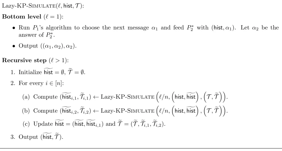
Lazy-KP Simulator. The rewinding strategy of the lazy-KP simulator is specified by the Lazy-KP-Simulate procedure. Very roughly, the simulator divides the current thread (given

as input) into n equal parts and then rewinds each part individually and recursively. The input to the Lazy-KP-Simulate procedure consists of a triplet (`,hist,T). The parameter ` denotes

the adversary’s messages to be explored, the string hist is a transcript of the current thread of execution, and T is a table containing the contents of all the adversary’s messages explored so far (to extract the preamble secrets and for sending the Stage 2 special message in protocol Π in any session).

The simulation is performed by invoking the procedure Lazy-KP-Simulate with appropriate

parameters. Letm=poly(n) denote the number of concurrent sessions in the adversarial schedule. Then, the Lazy-KP-Simulate procedure is invoked with input (m(N + 1),∅,∅), where m(N + 1)

is the total number of adversary’s messages in a schedule of m sessions. The Lazy-KP-Simulate

procedure is described in Figure1. Note that here (similar to [PPS+08]) we divide each thread into nparts. In other words, we consider a splitting factor of n.

Lazy-KP-Simulate(`,hist,T):

Bottom level(`= 1):

• Run P1’s algorithm to choose the next message α1 and feed P2∗ with (hist, α1). Let α2 be the

answer ofP2∗.

• Output ((α1, α2), α2).

Recursive step(` >1):

1. Initializeghist=∅, Te =∅. 2. For everyi∈[n]:

(a) Compute (histgi,1,Tei,1)←Lazy-KP-Simulate

`/n,hist,histg

,T,Te

.

(b) Compute (histgi,2,Tei,2)←Lazy-KP-Simulate

`/n,hist,histg

,T,Te

.

(c) Updateghist= (ghist,histgi,1) andTe = (Te,Tei,1,Tei,2).

3. Output (ghist,Te).

Figure 1: Lazy-KP Simulator with splitting factorn. Even though the messages in{ghisti,2}do not appear in the output, some of them do appear inTe.

For every session s consisting of an execution of Π, the goal of the simulator is to find two instances of any slot i∈ [N] of the commitment protocol hC, Ri where the simulator’s challenges are different and adversary responds with a valid response to each challenge. Note that in this case, the simulator can extract the preamble secret of hC, Ri from the two responses of the adversary. On the other hand, if the simulation reaches Stage 2 in Π at any time, without having extracted the preamble secret from the adversary, then it gives up the simulation and outputs ⊥. In this case, we say the simulatorgets stuck.

negligible probability.

Theorem 3 ([PTV14]). Let N = O(n). Then, for any concurrent schedule of m = poly(n) sessions, the lazy-KP simulator gets stuck with onlynegl(n) probability.

4.1 Terminology for Concurrent Simulation

Here we introduce some terminology and definitions regarding concurrent simulation that will be used in the rest of the paper.

Execution Thread. Consider any adversary that starts m = poly(n) number of concurrent sessions of Π. In order to extract the preamble secret in every session, the simulator creates multiple execution threads, where a thread of execution is a simulation of (part of) the protocol messages in the msessions. We differentiate between the following:

Main Thread vs Look-ahead Thread: Themain threadis a simulation of a complete execution of the m sessions, and this is the execution thread that is output by the simulator. In addition, from any execution thread, the simulator may create other threads by rewinding the adversary to a previous state and continuing the execution from that state. Such a thread is called a look-ahead thread. Note that a look-ahead thread can be created from another look-ahead thread.

Complete vs Partial Thread: We say that an execution thread T is a complete thread if it shares a prefix with the main thread: it starts where the main thread starts, and, continues until it is terminated by the simulator. Other threads that start from intermediary points of the simulation are calledpartialthreads. Note that by definition, the main thread is a complete thread. In general, a complete thread may consist of various partial threads. Various complete threads may overlap with each other. For simplicity of exposition, unless necessary, we will not distinguish between complete and partial threads in the sequel.

Simulation Transcript. The simulation transcript is the set of all the messages between the simulator and the adversary during the simulation of all the concurrent sessions. In particular, this includes the messages that appear on the main thread as well as all the look-ahead threads.

Simulation Index. Consider m = poly(n) concurrent executions of Π. Let M = m(2N + 2), where 2N + 2 is the round complexity of Π. Then, a simulation index i denotes the point where the i’th message (out of a maximum of M messages) is sent on any complete execution thread in the simulation transcript.

Note that a simulation index i may appearmultiple times on over various threads in the sim-ulation transcript. However, a simsim-ulation index i can appear at most once on any given thread (complete or partial). In particular, every simulation index i∈ [M] appears on the main thread (unless the main thread is aborted prematurely). Further, if a look-ahead thread T was created from a thread at simulation index i, then only simulation indicesj > i can appear on T.

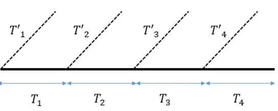
Figure 2: One recursion step for splitting factor 4. EveryTi and Ti0 are sibling threads.

schedule, protocol messages appear in thesame order on every complete thread. In particular, for every i ∈ [M], every instance of a simulation index i in the simulation transcript corresponds to thesame message indexj ∈[2N + 2] of the same session s(out of the m sessions). However note that the actual content of the j’th message may differ on every execution thread.

We say that a concurrent schedule is dynamicif at any point during the execution, the adver-sary may decide which message to schedule next based on the protocol messages received so far. Therefore, in a dynamic schedule, the ordering of messages may bedifferenton different execution threads in the simulation. In particular, each instance of a simulation indeximay correspond to a different message ji of adifferent session si.

Recursion Levels. We define recursion levels of simulation and count the number of threads at each recursion level for the lazy-KP simulator. We say that the main thread is at recursion level 0 of simulation. Note that the Lazy-KP-Simulatedivides the main thread of execution intonparts

and executes each part twice. This results in 2nexecution threads,nof which are part of the main thread, while the remaining n are look-ahead threads. All of these 2n threads are said to be at recursion level 1. Now, each of these threads at recursion level 1 is divided inton parts and each part is executed twice. This creates 2n threads at recursion level 2. Since there are 2n threads at recursion level 1, in total, we have (2n)2 threads at recursion level 2. (Again, out of these (2n)2 threads, 2n2 threads actually lie on the 2nthreads at level 1.) This process is continued recursively. At recursion level `, there are (2n)` threads. Since there are total m(2N + 2) messages across the m sessions, the depth of the recursion is a constant c0, where c0 =c+ log(2N+ 2) when m=nc. Then, at recursion level c0, there are (2n)c0 threads.

4.2 Analysis of λ for Static Schedules

We start by analyzing the lazy-KP extraction strategy for static schedules. Let λlazy-KP denote the

query parameter for the lazy-KP simulator. We claim the following:

Theorem 4. For any constantcand any concurrent execution ofm=nc instances of Πwhere the scheduling of messages is static, λlazy-KP = 2c

0

, where c0=c+ log(2N + 2). In order to prove Theorem 4, we will make use of the following lemma.

Lemma 1. For any constant c and any concurrent execution of m = nc instances of Π, the simulation transcript generated by the lazy-KP simulator is such that every simulation indexi∈[M] appears 2c0 times, where c0 =c+ log(2N + 2).

Proof. Fix any simulation indexi∈[M]. We will count the number of threads where iappears in the simulation transcript. We will use the definition of recursion levels for our analysis.

• First note that simulation index i appears exactly once on the main thread. Since main thread is the only thread at recursion level 0, we have thatiappears once at recursion level 0.

• Now, recall that there are 2n threads at recursion level 1. Then, the simulation index i appears on exactly 2 threads at recursion level 1 that are siblings of each other. To see this, recall that the Lazy-KP-Simulate procedure divides the main thread into n equal partsT1, . . . , Tn. Note that each of these parts corresponds to a thread at recursion level 1. Further, Lazy-KP-Simulate creates nlook-ahead threads T10, . . . , Tn0, one from each thread Ti, which contribute to the remainingn threads at recursion level 1. Now, since simulation indexiappears at most once on the main thread, letkbe such that indexiappears onTk(on the main thread). Then, note that amongst the set of look-ahead threads {T_j0}, simulation index ican only appear on T_k0 (which is a sibling of Tk). Thus, in total, simulation index i appears on 2 threads at recursion level 1.

• Now, suppose by induction hypothesis that the simulation indexiappears 2` times at recur-sion level`. LetT1, . . . , T₂` denote these 2`threads at recursion level`whereiappears. Now,

note that each of these threads Tj leads to 2n threads at recursion level`+ 1, out of which exactly 2 contain the simulation indexi. Thus, in total simulation indexiappears 2`+1 times at recursion level`+ 1.

• Finally, by induction, there are 2c0 appearances of simulation index i at the last recursion levelc0 =c+ log(2N + 2).

Now, note that in order the count the total number of different threads where the simulation indexiappears in the simulation transcript, we only need to count the number of times it appears at recursion level c0. This is because half of the 2c0 _{appearances of simulation index iat recursion} level c0 are on threads that are part of the threads at recursion level c0 −1. In particular, this is true for every recursion level`.

Proof of Theorem 4. Consider any sessions. From the definition of static scheduling, we have that for every j ∈ [2N+ 2], if the j’th message of session sappears at simulation index ion any thread, then every instance of simulation index i in the simulation transcript corresponds to the j’th message of session s. Now, from Lemma 1, since each simulation index appears 2c0 times in the simulation transcript, we have that the special message of every session sappears 2c0 times in the simulation. Thus, we have thatλlazy-KP= 2c

0

for static schedules.

4.3 Analysis of λ for Dynamic Schedules

We now analyze the query parameter λlazy-KP for the lazy-KP extraction strategy for dynamic

schedules. We claim the following:

Theorem 5. For any polynomial m=poly(n), for any concurrent execution of m instances of Π (with possibly dynamic scheduling of messages), λlazy-KP=O(logn) except with negligible

probabil-ity.

Proof of Theorem 5. Fix any session s out of the m = nc sessions. Note that the special messagemsg_sof sessionsappears exactly once on the main thread. Letimain denote the simulation

index wheremsg_s appears on the main thread. Now, we will count:

1. The number of times msg_s appears in the simulation transcript before imain. Let δ1 denote this number.

2. The number of timesmsg_s appears in the simulation transcript atimain orafterimain. Letδ2 denote this number.

Thus, the total number of times msg_s appears in the simulation transcript is δ1+δ2. In the rest of the proof, we will compute δ1 and δ2. In particular, we will show that (for every session s) δ1 +δ2 is bounded by O(logn) except with negligible probability. Note that this implies that λlazy-KP =O(logn).

Leti1, . . . , ikbe thedistinctsimulation indices wheremsgsappears in the simulation transcript. Let i1, . . . , ik be ordered, i.e., for every `∈[k−1], i` < i`+1. Let k1 ≤k be such that ik1 < imain and ik1+1 ≥imain. We first make the following claim:

Lemma 2. For any ` ∈ [k], the probability that msg<sub>s</sub> does not appear on the main thread at simulation index i` is at most (1− _c10).

Proof. Consider the simulation index i1. From Lemma 1, we have that i1 appears on 2c0 threads in the simulation transcript. LetT[i1] =T1, . . . , T₂c0 denote these threads. Now, letq be such that

the special message msg_s appears at simulation index i1 on q of these 2c0 threads. Let T∗[i1] = T₁∗, . . . , T_q∗ denote theseq threads. LetTmain denote the main thread. Then, we have that:

Pr [Tmain∈T∗[i1]] =

q

2c0 (1)

To see this, recall that the Lazy-KP-Simulate procedure uses uniformly random coins on each

appears onT0. (This is the “symmetry” property for threads in the lazy-KP simulation.) Therefore, Equation 1follows.

From Equation 1, we have that:

Pr [Tmain∈/T∗[i1]] = 1−

q 2c0

Note that the above probability is maximum when q= 1. Hence, we have that:

Pr[msg_s does not occur on main thread ati1]≤1− 1

2c0. (2)

Now, consider simulation indexi2. Again, from Lemma 1, we have thati2 appears on 2c0 threads. Let T[i2] denote the set of these threads. Now, note that msgs cannot appear on the look-ahead threadsT ∈T∗[i1]∩T[i2]. Thus, following Equation2, we have that:

Pr[msg_s does not occur on main thread ati2]≤1− 1

2c00.

wherec00 ≤c0. Continuing the same argument, we have that for every `∈[k−1],

Pr[msg_s does not occur on main thread at i`+1]≤Pr[msgs does not occur on main thread at i`]

Thus, for every i`, we have that the probability thatmsgs does not occur on main thread ati` is at most 1− _c10.

Computing δ1. Now, note that (1− _c10)t = negl(n) for t = ω(logn). Therefore, we have that

k1 = O(logn). Now, since each of the simulation indices i1, . . . , ik1 appears 2

c0 _{times in the}

simulation transcript, we have that:

δ1 ≤2c

0

O(logn) (3)

Computing δ2. We now compute the value of γ2. Towards this, let us suppose that for every simulation indexi∈[`], the Lazy-KP-Simulateprocedure runs all threads starting from simulation

index i in parallel. That is, Lazy-KP-Simulate performs one step of execution on each of these

threads. It then performs the next execution step on each of these threads, and so on. Note that this is without loss of generality since the Lazy-KP-Simulate procedure runs all such threads

independently.

Now, we first observe thatmsg_scannot appear on a look-ahead thread that starts at a simulation indexi > imain. Thus, to computeδ2, we only need to consider the look-ahead threads that started

at simulation indices i < imain and did not finish before reachingimain. LetTgood denote the set of

such threads.

Then, we claim that:

Lemma 3. |Tgood| ≤2c 0

.

Proof. Suppose for contradiction that |Tgood| >2c 0

. Now, by definition, each thread T ∈Tgood is

such that a simulation indexi≥imain appears on it. In other words, simulation indeximainappears

on each thread T ∈Tmain. However, from Lemma 1, simulation index imain appears on at most 2c 0

Now, assuming the worst case where msg_s appears on each threadT ∈Tgood, we have that:

δ2 ≤2c0 (4)

Completing the Proof of Theorem 5. From Equation3, we have thatδ1 =O(logn). From Equation

4, we have thatδ2 =O(1). Thus, summing upδ1 andδ2, we have that for every sessions, number of timesmsg_sappears in the simulation transcript isO(logn). Thus, we have thatλlazy-KP=O(logn).

This completes the proof.

5

GGJ Extraction Strategy

In this section, we discuss the GGJ extraction strategy [GGJ13] and analyze the query complexity parameter for the same. Unlike [GGJ13] that used a splitting factor of 2, we will work withnas the splitting factor. For this strategy, we will prove that for every concurrent schedule of polynomial number of sessions, the query parameterλ=O(1). Here, the constant inOdepends on the number of concurrent sessions.

We start by providing a brief overview of the GGJ extraction strategy. We then describe the GGJ strategy more formally and then proceed to analyze the query parameter λfor the same.

Overview. Roughly speaking, the GGJ rewinding strategy can be viewed as a “stripped down” version of the lazy-KP simulation strategy. In particular, unlike lazy-KP that executeseverythread at every recursion level, here we only execute a small fraction of them. The actual threads that are to be executed are chosen uniformly at random, at every level. It is shown in GGJ that by slightly increasing the round complexity – (roughly) N =n2 from N =n, executing a polylog_N n fraction of threads at every level is sufficient to extract the preamble secret in every session.5

Below, we describe the GGJ rewinding strategy in two main steps:

1. We first describe an algorithmSparsifythat essentially selects which threads to execute in the lazy-KP recursion tree (Section5.1).

2. Next, we describe the actual GGJ simulation procedure GGJ-Simulate that is essentially

the same as the Lazy-KP-Simulatestrategy, except that it only executes the threads selected

by Sparsify (Section5.2).

5.1 The Sparsification Procedure

We first describe the lazy-KP simulation tree and give a coloring scheme for the same. Next, we describe the Sparsify algorithm that takes the lazy-KP simulation tree as input and outputs a “trimmed” version of it that will correspond to the GGJ simulation tree.

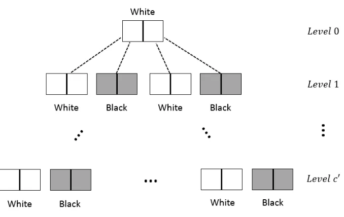
Lazy-KP Simulation Tree. Letm=ncbe the total number of concurrent sessions of Π started by an adversary A. Then, the Lazy-KP-Simulate strategy for A can be described by a 2n-ary

treeTreelazy-KPof constant depthc0 wherec0 =c+ log(2N+ 2). The nodes inTreelazy-KP are colored

white orblackas per the following strategy:

5

Figure 3: The lazy-KP simulation tree for splitting factor 2.

• The root node is colored white.

• Consider the 2nchild nodes of any parent node. The odd numbered nodes are colored white and the even numbered nodes are colored black.

Let us explain our coloring strategy. The root node (which is colored white) corresponds to the main thread of execution. Each black colored node Nodecorresponds to a look-ahead thread that was forked from the thread corresponding to nodeParent(Node). A white colored nodeNode(except the root node) corresponds to a thread T0 that is a part of the thread T corresponding to node Parent(Node).

Figure 3denotes the lazy-KP simulation tree for splitting factor n= 2 with white boxes repre-senting white nodes and grey boxes reprerepre-senting black nodes.

Node Labeling. To facilitate the description of the GGJ simulation strategy, we first describe a simple tree node labeling strategy forTreelazy-KP. The root node is labeled 1. Thei’th child (out of

2nchildren) of the root node is labeled (1, i). More generally, consider a nodeNodeat level`∈[c0]. Letpathbe its label. Then the i’th child of Nodeis labeled (path, i).

Below, whenever necessary, we shall refer to the nodes by their associated labels.

The Sparsify Procedure. Letpbe such that 1_p = polylog_N (n). TheSparsifyfunction transforms the lazy-KP simulation tree Treelazy-KP into a “sparse” treeTreesp in the following manner.

Let the root node correspond to level 0 and the leaf nodes correspond to level c0. The Sparsify procedure starts at level 0 and traverses down Treelazy-KP, stopping at level c0. It performs the

1. Choose 1_p fraction of the total black nodes at level`, uniformly at random. LetB` denote the set of these nodes.

2. Delete fromTreelazy-KP, every black nodeNodeat level`that is not present in setB`. Further, delete the entire subtree ofNode fromTreelazy-KP.

The resultant tree is denoted as Treesp. Looking ahead, we will describe the GGJ rewinding

strategy as essentially a modification of Lazy-KP-Simulate in that it only executes the threads

corresponding to the nodes inTreesp.

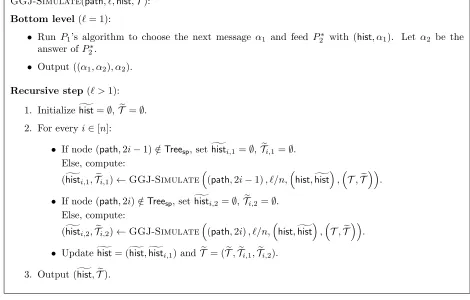
5.2 The GGJ-Simulate Procedure

The rewinding strategy of the GGJ simulator is specified by the GGJ-Simulate procedure. The

input to the GGJ-Simulate procedure consists of a tuple (path, `,hist,T). The parameter path

denotes the label of the node inTreesp that is to be explored,` denotes the number of adversary’s

messages to be explored (on the thread corresponding to the node labeled with path), the string histis a transcript of thecurrentthread of execution,T is a table containing the contents of all the adversary’s messages explored so far (to extract the preamble secrets and for sending the Stage 2 special message in Π in any session).

The simulation is performed by invoking the procedure GGJ-Simulate with appropriate

pa-rameters. Let m =poly(n) denote the number of concurrent sessions in the adversarial schedule. Then, theGGJ-Simulate procedure is invoked with input (1, m(N+ 1),∅,∅), wherem(N+ 1) is

the total number of adversary’s messages in a schedule ofm sessions. TheGGJ-Simulate

proce-dure is described in Figure 4. Note that unlike [GGJ13], where each thread is recursively divided into two parts, here we divide each thread into n parts. In other words, we consider a splitting factor of n. For every session s consisting of an execution of Π, the goal of the simulator is to find two instances of any slot i ∈ [N] of the commitment protocol hC, Ri where the simulator’s challenges are different and adversary responds with a valid response to each challenge. Note that in this case, the simulator can extract the preamble secret ofhC, Rifrom the two responses of the adversary. On the other hand, if the simulation reaches Stage 2 in Π at any time, without having extracted the preamble secret from the adversary, then it gives up the simulation and outputs ⊥. In this case, we say the simulator gets stuck.

It is implicit in [GGJ13] that the GGJ simulator (as described above) gets stuck with only negligible probability whenN =O(n2).

Theorem 6([GGJ13]). LetN =O(n2)be the number of slots inhC, Ri. Then, for any concurrent schedule of m=poly(n) sessions of Π, the GGJ simulator gets stuck with only negl(n) probability.

We now analyze the query parameter λGGJ for the GGJ simulation strategy. We claim the

following:

Theorem 7. For every constant c, everym=nc _{number of concurrent executions of Π, the query} parameter λGGJ =O(1), where the constant depends on c.

Proof. Fix any session s. We will show that the special message msg_s can appear at most O(1) times at each recursion levelRL`. Then, since there are only a constant number of recursion levels, it will follow thatλGGJ=O(1).

GGJ-Simulate(path, `,hist,T):

Bottom level(`= 1):

• Run P1’s algorithm to choose the next message α1 and feed P2∗ with (hist, α1). Let α2 be the

answer ofP2∗.

• Output ((α1, α2), α2).

Recursive step(` >1):

1. Initializeghist=∅, Te =∅. 2. For everyi∈[n]:

• If node (path,2i−1)∈/ Treesp, sethistgi,1=∅,Tei,1=∅.

Else, compute:

(ghisti,1,Tei,1)←GGJ-Simulate

(path,2i−1), `/n,hist,histg

,T,Te

.

• If node (path,2i)∈/Treesp, set histgi,2=∅,Tei,2=∅.

Else, compute:

(ghisti,2,Tei,2)←GGJ-Simulate

(path,2i), `/n,hist,histg

,T,Te

.

• Updateghist= (ghist,histgi,1) andTe = (Te,Tei,1,Tei,2).

3. Output (ghist,Te).

Figure 4: GGJ Simulator with splitting factor n. Even though the messages in {ghisti,2} do not appear in the output, some of them do appear inTe.

the lazy-KP simulation, msg_s for a sessions appears on at most O(logn) threads. Using the tree terminology as introduced earlier, we have thatmsg_s appears on (the threads corresponding to) at most O(logn) black nodes at level ` in Treelazy-KP. Now, recall that at every level `, theSparsify

procedure selects only 1_p = polylog_N n fraction of black nodes, uniformly at random, and deletes the rest of the black nodes. Using Chernoff bound, we now show that the probability that Sparsify selectsω(1) black nodes containing msg_s is negligible.

Towards that end, first note that the expected number of black nodes selected by Sparsify that contain the heavy messagemsg_s isµ= polylog_N n· O(logn). Let γ denote the actualnumber of black nodes at level` containingmsg_s that are selected by Sparsify. Then, we have that:

Pr[λ≥(1 +δ)µ]≤

eδ (1 +δ)1+δ

µ

(5)

the fact that 1 +δ ≈δ and substituting values in Equation 5, we have:

Pr[γ ≥ω(1)] ≤ 

  

e

ω(1)·N

polylogn

ω(1)·N

polylogn

_polylogω(1)·N_n 

  

polylogn N

≤

polylogn N

ω(1)

= negl(n)

when N = O(n). Thus, for every level `, we have γ = O(1). It then follows that λGGJ = O(1).

6

From Concurrent Extraction to Concurrently Secure

Computa-tion

Theorem 8. Assuming 1-out-of-2 oblivious transfer, for any efficiently computable functionalityf there exists a protocol Π thatO(1)-securely realizes f in the MIQ model.

We construct such a protocol by following the exact recipe of [GJO10,GGJ13]. We note that the works of [GJO10, GGJ13] show how to compile a semi-honest secure computation protocol Πsh for any functionalityf into a new protocol Π that securely realizes f in the MIQ model (we

discuss the query parameter λ shortly). The core ingredient of their compiler is a concurrently extractable commitment hC, Ri, which in turn is used inside a concurrent non-malleable zero-knowledge protocol. In particular, it follows from these works that if there exists a concurrent simulator for hC, Ri with query parameter λ, then the resultant (compiled) protocol Π λ-securely realizesf.

Then, in order to prove Theorem 8, we construct such a protocol Π by simply plugging in our O(n2)-round extractable commitment scheme in the construction of [GJO10,GGJ13]. Then, it follows from Theorem 7 that protocol Π O(1)-securely realizes f in the MIQ model, where the constant inOdepends onc, wherencis the number of sessions opened by the concurrent adversary. For completeness, we provide a description of protocol Π in Appendix A (which remain identical to these prior works except for the concurrently extractable commitment scheme being used).

References

[AGJ+12] Shweta Agrawal, Vipul Goyal, Abhishek Jain, Manoj Prabhakaran, and Amit Sahai. New impossibility results on concurrently secure computation and a non-interactive completeness theorem for secure computation. In CRYPTO, 2012.

[BCNP04] B. Barak, R. Canetti, J.B. Nielsen, and R. Pass. Universally composable protocols with relaxed set-up assumptions. In FOCS, 2004.

[Blu87] Manual Blum. How to prove a theorem so no one else can claim it. In International Congress of Mathematicians, pages 1444–1451, 1987.

[BPS06] Boaz Barak, Manoj Prabhakaran, and Amit Sahai. Concurrent non-malleable zero knowledge. In FOCS, 2006.

[BS05] Boaz Barak and Amit Sahai. How to play almost any mental game over the net -concurrent composition using super-polynomial simulation. In Proc.46th FOCS, 2005.

[CF01] Ran Canetti and Marc Fischlin. Universally composable commitments. In CRYPTO, 2001.

[CKL03] Ran Canetti, Eyal Kushilevitz, and Yehuda Lindell. On the limitations of universally composable two-party computation without set-up assumptions. In Eurocrypt, 2003.

[CKPR01] Ran Canetti, Joe Kilian, Erez Petrank, and Alon Rosen. Black-box concurrent

zero-knowledge requires Ω (log∼ n) rounds. In STOC, pages 570–579, 2001.

[CLOS02] R. Canetti, Y. Lindell, R. Ostrovsky, and A. Sahai. Universally composable two-party and multi-party secure computation. InSTOC, 2002.

[CLP10] Ran Canetti, Huijia Lin, and Rafael Pass. Adaptive hardness and composable security in the plain model from standard assumptions. In FOCS, 2010.

[DDN00a] Danny Dolev, Cynthia Dwork, and Moni Naor. Nonmalleable cryptography. SIAM Journal on Computing, 30(2):391–437 (electronic), 2000. Preliminary version in STOC 1991.

[DDN00b] Danny Dolev, Cynthia Dwork, and Moni Naor. Nonmalleable cryptography. SIAM J. Comput., 30(2):391–437, 2000.

[DNS98] Cynthia Dwork, Moni Naor, and Amit Sahai. Concurrent zero-knowledge. In STOC, pages 409–418, 1998.

[GGJ13] Vipul Goyal, Divya Gupta, and Abhishek Jain. What information is leaked under concurrent composition. In CRYPTO, 2013.

[GGJS12] Sanjam Garg, Vipul Goyal, Abhishek Jain, and Amit Sahai. Concurrently secure com-putation in constant rounds. InEurocrypt, 2012.

[GJO10] Vipul Goyal, Abhishek Jain, and Rafail Ostrovsky. Password-authenticated session-key generation on the internet in the plain model. CRYPTO, 2010. Full version available online.

[GK96] Oded Goldreich and Hugo Krawczyk. On the composition of zero-knowledge proof systems. SIAM Journal on Computing, 25(1):169–192, February 1996. Preliminary version appeared in ICALP’ 90.

[GKOV12] Sanjam Garg, Abishek Kumarasubramanian, Rafail Ostrovsky, and Ivan Visconti. Im-possibility results for static input secure computation. In CRYPTO, 2012.

[GL01] Oded Goldreich and Yehuda Lindell. Session-key generation using human passwords only. In CRYPTO, pages 408–432, 2001.

[GL06] Oded Goldreich and Yehuda Lindell. Session-key generation using human passwords only. J. Cryptology, 19(3):241–340, 2006.

[GMW87] O. Goldreich, S. Micali, and A. Wigderson. How to play any mental game. InSTOC, 1987.

[Goy12] Vipul Goyal. Positive results for concurrently secure computation in the plain model. In FOCS, 2012.

[HHK+_{05] Iftach Haitner, Omer Horvitz, Jonathan Katz, Chiu-Yuen Koo, Ruggero Morselli, and} Ronen Shaltiel. Reducing complexity assumptions for statistically-hiding commitment. In Eurocrypt, pages 58–77, 2005.

[Kat07] J. Katz. Universally composable multi-party computation using tamper-proof hardware. In Eurocrypt, 2007.

[Kil88] Joe Kilian. Founding cryptography on oblivious transfer. InSTOC, pages 20–31, 1988.

[KP01] Joe Kilian and Erez Petrank. Concurrent and resettable zero-knowledge in poly-loalgorithm rounds. In STOC, 2001.

[Lin03] Yehuda Lindell. Bounded-concurrent secure two-party computation without setup as-sumptions. InSTOC, pages 683–692. ACM, 2003.

[MP06] Silvio Micali and Rafael Pass. Local zero knowledge. In STOC, 2006.

[MPR06] Silvio Micali, Rafael Pass, and Alon Rosen. Input-indistinguishable computation. In FOCS, 2006.

[Nao91] Moni Naor. Bit commitment using pseudorandomness. J. Cryptology, 4(2):151–158, 1991.

[NOVY98] Moni Naor, Rafail Ostrovsky, Ramarathnam Venkatesan, and Moti Yung. Perfect zero-knowledge arguments forNP using any one-way permutation. J. Cryptology, 11(2):87– 108, 1998.

[NP06] Moni Naor and Benny Pinkas. Oblivious polynomial evaluation. SIAM J. Comput., 35(5):1254–1281, 2006.

[Pas03] Rafael Pass. Simulation in quasi-polynomial time, and its application to protocol com-position. InEurocrypt, 2003.

[PPS+08] Omkant Pandey, Rafael Pass, Amit Sahai, Wei-Lung Dustin Tseng, and Muthuramakr-ishnan Venkitasubramaniam. Precise concurrent zero knowledge. InEurocrypt, 2008.

[PRS02] Manoj Prabhakaran, Alon Rosen, and Amit Sahai. Concurrent zero knowledge with logarithmic round-complexity. In FOCS, 2002.

[PS04] Manoj Prabhakaran and Amit Sahai. New notions of security: achieving universal composability without trusted setup. InSTOC, 2004.

[PTV14] Rafael Pass, Wei-Lung Dustin Tseng, and Muthuramakrishnan Venkitasubramaniam. Concurrent zero knowledge, revisited. Journal of Cryptology, 27(1):45–66, 2014.

[RK99] Ransom Richardson and Joe Kilian. On the concurrent composition of zero-knowledge proofs. InEurocrypt, 1999.

[Yao86] Andrew Chi-Chih Yao. How to generate and exchange secrets. In FOCS, 1986.

A

The Protocol

In this section, we describe our concurrently secure computation protocol Π in the MIQ model for a general functionality F. We remark that this protocol is exactly the same as the one presented in [GJO10,GGJ13] except that we shall use anN =O(n2_{)-round version of the extractable} com-mitment scheme hC, Ri (Section 3.1), while [GJO10, GGJ13] require different round-complexities forhC, Ri.

We start by recalling the building blocks used in the protocol.

A.1 Building Blocks

A.1.1 Statistically Binding String Commitments

In our protocol, we will use a (2-round) statistically binding string commitment scheme, e.g., a parallel version of Naor’s bit commitment scheme [Nao91] based on one-way functions. For simplicity of exposition, in the presentation of our results, we will actually use a non-interactive perfectly binding string commitment.6 Such a scheme can be easily constructed based on a 1-to-1 one way function. Letcom(·) denote the commitment function of the string commitment scheme.

For simplicity of exposition, in the sequel, we will assume that random coins are an implicit input to the commitment function.

6_{It is easy to see that the construction given in SectionA does not necessarily require the commitment scheme}

A.1.2 Statistically Witness Indistinguishable Arguments

In our construction, we shall use a statistically witness indistinguishable (SWI) argumenthPswi, Vswii

for proving membership in any NP language with perfect completeness and negligible soundness error. Such a scheme can be constructed by using ω(logk) copies of Blum’s Hamiltonicity proto-col [Blu87] in parallel, with the modification that the prover’s commitments in the Hamiltonicity protocol are made using a statistically hiding commitment scheme [NOVY98,HHK+05].

A.1.3 Semi-Honest Two Party Computation

We will also use a semi-honest two party computation protocol hPsh

1 , P2shi that emulates the func-tionalityF (as described in section 2) in the stand-alone setting. The existence of such a protocol

hP₁sh, P₂shifollows from [Yao86,GMW87,Kil88].

A.1.4 Concurrent Non-Malleable Zero Knowledge Argument

Concurrent non-malleable zero knowledge (CNMZK) considers the setting where a man-in-the-middle adversary is interacting with several honest provers and honest verifiers in a concurrent fashion: in the “left” interactions, the adversary acts as verifier while interacting with honest provers; in the “right” interactions, the adversary tries to prove some statements to honest verifiers. The goal is to ensure that such an adversary cannot take “help” from the left interactions in order to succeed in the right interactions. This intuition can be formalized by requring the existence of a machine called the simulator-extractor that generates the view of the man-in-the-middle adversary and additionally also outputs a witness from the adversary for each “valid” proof given to the verifiers in the right sessions.

Barak, Prabhakaran and Sahai [BPS06] gave the first construction of a concurrent non-malleable zero knowledge (CNMZK) argument for every language in NP with perfect completeness and negligible soundness error.

In our main construction, we will use a specific CNMZK protocol, denoted hP, Vi, based on the CNMZK protocol of Barak et al. [BPS06] to guarantee non-malleability. Specifically, we will make the following two changes to Barak et al’s protocol: (a) Instead of using an ω(logn)-round extractable commitment scheme [PRS02], we will use theN-round extractable commitment scheme

hC, Ri (described in Section 3.1). (b) Further, we require that the non-malleable commitment scheme being used in the protocol be public-coin w.r.t. receiver7. We now describe the protocol

hP, Vi.

Protocol hP, Vi. LetP and V denote the prover and the verifier respectively. Let L be an NP language with a witness relation R. The common input to P and V is a statement x ∈ L. P additionally has a private input w (witness for x). Protocol hP, Vi consists of two main phases: (a) the preamble phase, where the verifier commits to a random secret (say) σ via an execution of

hC, Riwith the prover, and (b) thepost-preamble phase, where the prover proves an NP statement. In more detail, protocol hP, Vi proceeds as follows.

7_{The original NMZK construction only required a public-coin extraction phase inside the non-malleable}

Preamble Phase.

1. P andV engage in execution ofhC, Ri (Section3.1) where V commits to a random string σ.

Post-preamble Phase.

2. P commits to 0 using a statistically-hiding commitment scheme. Letc be the commitment string. Additionally,P proves the knowledge of a valid decommitment tocusing a statistical zero-knowledge argument of knowledge (SZKAOK).

3. V now reveals σ and sends the decommitment information relevant to hC, Ri that was exe-cuted in step 1.

4. P commits to the witnessw using a public-coin non-malleable commitment scheme.

5. P now proves the following statement toV using SZKAOK:

(a) either the value committed to in step 4 is a valid witness tox (i.e., R(x, w) = 1, where w is the committed value),or

(b) the value committed to in step 2 is the trapdoor secretσ.

P uses the witness corresponding to the first part of the statement.

A.1.5 Modified Extractable Commitment Scheme hC0, R0i

Due to technical reasons, in our secure computation protocol, we will also use a minor variant, denoted hC0, R0i, of the extractable commitment scheme given in Section 3.1. Protocol hC0, R0i

is the same as hC, Ri, except that for a given receiver challenge string, the committer does not “open” the commitments, but instead simply reveals the appropriate committed values (without revealing the randomness used to create the corresponding commitments). More specifically, in protocolhC0, R0i, on receiving a challenge stringvj =v1,j, . . . , v`,j from the receiver, the committer uses the following strategy: for everyi∈[`], ifvi,j = 0,C0 sendsα0i,j, otherwise it sends α1i,j toR0. Note thatC0 does not reveal the decommitment values associated with the revealed shares.

When we use hC0, R0i in our main construction, we will require the committer C0 to prove the “correctness” of the values (i.e., the secret shares) it reveals in the last step of the commitment protocol. In fact, due to technical reasons, we will also require the the committer to prove that the commitments that it sent in the first step are “well-formed”.

We remark that the extraction proofs for the Lazy-KP-Simulate procedure (Section 4) and GGJ-Simulateprocedure (Section 5) also hold for thehC0, R0i commitment scheme.

A.2 Protocol Description

Notation. Let com(·) denote the commitment function of a non-interactive perfectly binding

commitment scheme. LethC, Ridenote theN-round extractable commitment scheme andhC0, R0i

be its modified version as described in Section A.1.5. Let hP, Vi denote the modified version of the CNMZK argument of Barak et al. [BPS06] as described in Section A.1.4. Further, let

hPswi, Vswii denote a SWI argument (Section A.1.2) and let hP1sh, P2shi denote a semi-honest two party computation protocol hP₁sh, P₂shi that securely computesF in the stand-alone setting as per the standard definition of secure computation (SectionA.1.3).

I. Trapdoor Creation Phase.

1. P1 ⇒ P2 : P1 creates a commitment com1 =com(0) to bit 0 and sendscom1 toP2. P1 and P2 now engage in the execution of hP, Viwhere P1 proves thatcom1 is a commitment to 0.

2. P2 ⇒ P1 :P2 now acts symmetrically. That is, it creates a commitmentcom2 =com(0) to bit 0 and sendscom2 toP1. P2andP1 now engage in the execution ofhP, ViwhereP2 proves thatcom2 is a commitment to 0.

Informally speaking, the purpose of this phase is to aid the simulator in obtaining a “trapdoor” to be used during the simulation of the protocol.

II. Input Commitment Phase. In this phase, the parties commit to their inputs and random coins (to be used in the next phase) via the commitment protocolhC0, R0i.

1. P1 ⇒ P2 : P1 first samples a random string r1 (of appropriate length, to be used as P1’s randomness in the execution ofhP₁sh, P₂shiin Phase III) and engages in an execution ofhC0, R0i

(denoted as hC0, R0i1→2) with P2, where P1 commits to x1kr1. Next, P1 and P2 engage in an execution of hPswi, Vswii where P1 proves the following statement to P2: (a) either there exist values ˆx1, ˆr1 such that the commitment protocolhC0, R0i1→2 isvalid with respect to the value ˆx1kr1ˆ,or (b)com1 is a commitment to bit 1.

2. P2 ⇒ P1 :P2 now acts symmetrically. Let r2 (analogous tor1 chosen byP1) be the random string chosen byP2 (to be used in the next phase).

Informally speaking, the purpose of this phase is aid the simulator in extracting the adversary’s input and randomness.

III. Secure Computation Phase. In this phase,P1andP2engage in an execution ofhP1sh, P2shi whereP1plays the role ofP₁sh, whileP2plays the role ofP₂sh. SincehP₁sh, P₂shiis secure only against semi-honest adversaries, we first enforce that the coins of each party are truly random, and then executehPsh

1 , P2shi, where with every protocol message, a party gives a proof usinghPswi, Vswii of its

honest behavior “so far” in the protocol. We now describe the steps in this phase.

1. P1 ↔P2 :P1 samples a random stringr02(of appropriate length) and sends it toP2. Similarly, P2 samples a random string r10 and sends it to P1. Letr100=r1⊕r10 and r002 =r2⊕r02. Now, r₁00 and r00₂ are the random coins thatP1 andP2 will use during the execution ofhP₁sh, P₂shi. 2. Lettbe the number of rounds inhP₁sh, P₂shi, where one round consists of a message fromP₁sh

followed by a reply from P₂sh. Let transcript T1,j (resp., T2,j) be defined to contain all the messages exchanged between P₁sh and P₂sh before the point P₁sh (resp., P₂sh) is supposed to send a message in roundj. Forj= 1, . . . , t:

(a) P1 ⇒P2: Computeβ1,j =P1sh(T1,j, x1, r001) and send it to P2. P1 and P2 now engage in an execution ofhPswi, Vswii, whereP1 proves the following statement:

i. either there exist values ˆx1, ˆr1 such that (a) the commitment protocolhC0, R0i1→2 isvalid with respect to the value ˆx1krˆ1, and (b) β1,j =P1sh(T1,j,xˆ1,rˆ1⊕r10)

ii. or,com1 is a commitment to bit 1. (b) P2 ⇒P1 :P2 now acts symmetrically.